Flood Mitigation of Nyando River Using Duflow Modelling
Joleha, J.1, Maino, V.2, Adyabadam, A.3, Zhao, W.4, Ke, S.4, and Le, T. H.5
Abstract: Duflow surface water hydrodynamic model has been applied using a case study from Nyando catchment in the western part of Kenya in Africa to simulate various extreme flood behaviours and their retardation levels by using selected structural measures as flood mitigation techniques. The objective of this case study was to establish a design flood recommendable for mitigation, and to identify the most cost effective flood mitigation structure. Various design flows are simulated against the different proposed structures hence, the optimal structure can be recommended when economical, social and environmental constraints are considered in the decision making process. The proposed four flood mitigation structures flood plain extension, embankment (dykes), channel by-pass, and green-storage were simulated for 20-year recurrence interval flood to determine their individual responses in storing excess water. The result shows that building a green-storage is the best and optimal structure for flood mitigation.
Keywords: Duflow, Flood mitigation.
Introduction
Flood plain flooding is a major phenomenon in many meandering and alluvial rivers. Situations can become worst by rapid population growth and increasing urbanisation. The need for the rural population to live within the proximities of the river banks which are flood prone areas can often be influenced by the need to have rapid access to drinking water supply, irrigation and livestock grazing. Hazards arising from extreme water movement are never considered.
Nyando catchment is an ideal source of subsistence farming, rice cultivation, cattle grazing, drinking water supply, irrigation, and navigation. On the other hand it is also a discharge point for all organic and inorganic matter, and pollution from the sugar mill which is a major concern. It has an area of 3587 km2, and is located in the western part of Kenya in Africa. The location at Ahero is 340 56’East and 00 10’South. Conceptually, it is a sub catchment of Lake Victoria, enveloping an area of 194000 km2 [1].
1Civil Engineering Departement, Faculty of Engineering, Riau University, Pekanbaru, Indonesia.
Email: joleha@unri .ac.id
2 Depart. of Environment and Conservation, PO.BOX 6580, BOROKO National Capital PNG
3 Institute of Meteorology and Hydrology, Researcher UB. Mongolia 4Hydrological Bureau of Yellow River Conservation Commission, China
5 The Institue of Water Resources Planning, 164a Tiang Quang Khai, Hanoi, Vietnam
Note: Discussion is expected before June, 1st 2009, and will be published in the “Civil Engineering Dimension” volume 11, number 2, September 2009.
Received 8 September 2008; revised 4 December 2008; accepted 16 February 2009.
To maintain consistency, Nyando sub catchment will be referred to as a catchment in this report. Figure 1 shows the elevation contours of the Nyando catch-ment.
The Nyando catchment is categorised into three main sub catchments, comprising of;
(a)Ainmotua in the north (200 km2), sloping from eats to the west,
(b)Kipchoriet in the central (1712 km2), sloping from east to west, and
(c) Cherongit and Kabletach with minor stream (888 km2), sloping southeast to northwest [2].
The average elevation is more than +1600 m above sea level, and predominantly receives 1500–1700 mm per year. Small-scale dams have been con-structed upstream to trap the overland runoff. During the monsoon period (February-April, October-December) extreme flood is experienced with devastating effects on the population inhabiting the Kano flood plains. Because the Nyando flow velocities are high during peak flows, high volume of water and sediment is transported and deposited into the lake. This indicates that the riverbed is prone to erosion, and subsequently giving rise to the meandering process.
Average rainfall in the catchment, based on the data obtained from the Kenya Meteorological Department is varying from 1000 mm in the Kano plain to 1600 mm at the base of Nyando escarpment. The mean annual temperature is estimated to be 23 0C [3] with annual mean rainfall of 1184 mm.
The soil are predominantly vertisol type, grey to black in colour, with a single clayey profile, and the entosol type which are clayey but showing signs of re-adjustment due to the movement of surface waters [4]. Ainmotua stream flows to North of Tinderet along the Nyando catchment . The stream is originating from the lake Nandi. Predominant streams are the Ainopsiwa, Kapchure and Mbogo.
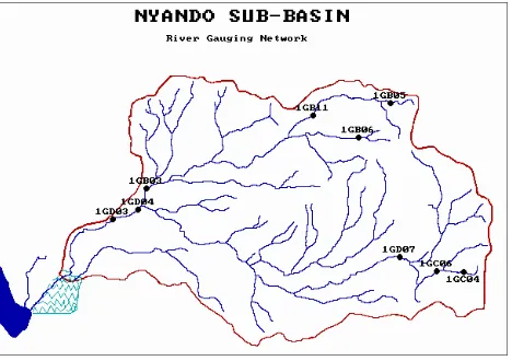
The Tinderet forest in the Northeast and the Mau forest in Kericho in the South are the upper Nyando tributaries. Figure 2 shows the drainage network. The confluence of Ainomotua with Nyando is approximately 1 km south of Kimbigori. At this point the river incises a channel of 12m through the alluvial soil that forms the rapid banks. Land utilisation is dominated by food cropping, and grazing. Common subsistence crops such as corn (maize), beans and sorghum are prevalent in the North. Cash cropping practice is common in the South, where rice and cotton are the dominant crops. Patches of cattle grazing can be found but not very intense.
The objective of this case study was to establish a design flood recommendable for mitigation, and to identify the most cost effective flood mitigation
structure. Various design flows are simulated against the different proposed structures, then the optimal structure is finally recommended after economical, social and environmental constraints are considered in the decision making process.
Material and Methods
Data interpretation and analysis was performed, using standard statistical procedures and tests. Missing data is then filled in as and when appropriate. Preliminary steps include testing of trends, homogeneity and consistency, establishing correlation between stations, defining relationship between rainfall and discharge, sorting extreme data, and finally executing the flood frequency analysis.
Duflow surface water hydrodynamic model [5] is used in this case study to simulate various extreme flood behaviours, and their retardation levels using four structural measures; flood plain extension, embankment (dykes), channel by-pass, and green-storage, as flood mitigation techniques. Essential requirements include river and bed levels, channel roughness, river cross-sections, boundary and initial conditions.
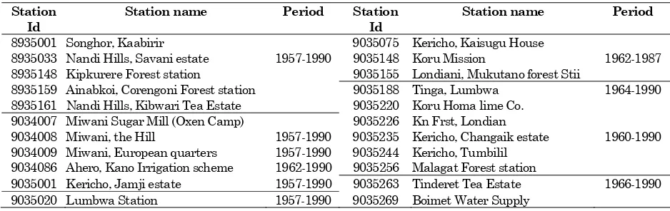
Calibration of the design storm was done using the inflows from the tributaries and compared against the observed data. Conversion factors were applied to the observed storm to emulate the desired boundary condition at Ahero. The behaviours of the proposed flood mitigation structures were then evaluated. The Kenya Ministry of Water Resource supplies the daily discharge and rating curve data for nine monitoring stations, distributed from 1959-1997 [1], as shown in Table 1.
The rainfall data are provided by the Department of Meteorology, Ministry of Information and Ministry of Transport and Communication [1]. Table 2 provides the list of rainfall and their period of records. Topographical and geological maps of 1:100000 scales were obtained but some vital sheets were found to be missing.
Gauging station 1GDO3 at Ahero was established in 1969 and installed with an automatic water level recorder and cableway for flood gauging. The period of daily discharge records is from 1969 to 1990, with discharges ranging from 0.004 m3/s to 688.931 m3/s. The average daily discharge is 17.600 m3/s. The cross-section depths range from 0.0 m at the floor (bed) level to 12.0 m at the land surface (banks). The width of the cross section extends from 30 m at the floor level to approximately 80 meters at the land surface. The gauged flows are valid up to at 5.03 m only.
Data Analysis
Prior to the commencement of water level and discharge simulation using the Duflow surface water hydrodynamic model, the authenticity of the raw data had to be corroborated. Using the Microsoft Figure 2.: Drainage system and discharge station [1]
Table 1. Discharge monitoring stations Station
Id
Location Period of
record
Station Id
Location Period of
record
1GB11 Upstream Kigwan 1959-1995 1GB05 Nyando, upstream 1950-1989
1GD03* Upstream Ahero 1969-1996 1GB06 Mbogo 1950-1988
1GD04 Nyando, downstream junction 1956-1990 1GC04 Tugenon 1959-1992
1GD07 Nyando, upstream 1963-1997 1GC06 Nyando, upstream 1967-1989
1GB03 Ainomutua, upstream 1967-1990 -
Excel spreadsheet, discharge, water level and rain-fall data provided were put through vigorous statistical tests.
Potential forms of error
Double mass curve.One of the methods used was plotting the cumulative discharges and rainfall against neighbouring stations. The concept was to identify any breaking points in between the data series and if such case existed correction by multiple regression models was performed. The causes of the diverting points were not investigated; nevertheless corrections were applied to create complete set of records for our analysis. Many rainfall stations showed more than two breaking points. Changes in land use and urbanisation, changes in instrument-tation, observation times and personnel over the years are alleged to be some of the factors attributing to theses break points.
Simple mass balance. Reference station 1GD03 in theory should accumulate flows originating from the upstream. Discharge measured in 1GD03 should be equal to discharge measure in 1GD04, which is a sum of discharges from 1GB03, 1GD02 and a small tributary between the two stations. However, it was verified that this may true for dry weather flows, but may not necessarily true for wet season since there is lateral inflow and surface water runoff. At times flow in station 1GB04 (upstream) were greater than flows recorded in station 1GD03 (downstream). Two major assumptions can be attributed to inaccuracies in flow gauging measurements, and inconsistencies in the bed levels caused by sedimentation process.
Extreme discharges. Design floods are extracted from either annual flow series or from peaks above a certain threshold. The former is just taking one extreme value in one single year, while the latter refers to selecting a number of flows over given threshold from a population of extreme discharges. The only difficulty encountered in the latter case was
when multiple peaks occurred in a single storm event, that is deciding which peak represented what flood event. Moreover, more than two peaks selected from one year while no peak above a prescribed threshold is registered in other years did not provide a truly representative annual extreme series.
Univariate description. Univariate tools can be used to describe the distribution of the individual variable. The most common tool is histogram, which record how often observation values fall within a certain class. The class width is normally constant so that the height of each bar is proportional to the number of observations. The features of the histogram can be interpreted by the following statistics.
• Descriptors of central tendency: Parameters indicating the central or most typical value around which other values cluster are descriptors to measure the central tendency of a variable. Descriptors of the central tendency are often referred to as averages. And the mean is the most commonly used measured of the central tendency. the data values.
• Descriptors of dispersion: Dispersion parameters measure how the variable values are dispersed or spread out about a central value. In which the variance (S2) indicates the dispersion of the variable values around the mean.
( )
Standard deviation (S) is the square root of the variance and the coefficient of variation is defined as the ratio of the standard deviation to the mean:
x S
Cv = (3)
Table 2. Rainfall Monitoring stations Station
Id
Station name Period Station Id
Station name Period
8935001 Songhor, Kaabirir 9035075 Kericho, Kaisugu House
8935033 Nandi Hills, Savani estate 1957-1990 9035148 Koru Mission 1962-1987 8935148 Kipkurere Forest station 9035155 Londiani, Mukutano forest Stii
8935159 Ainabkoi, Corengoni Forest station 9035188 Tinga, Lumbwa 1964-1990 8935161 Nandi Hills, Kibwari Tea Estate 9035220 Koru Homa lime Co.
9034007 Miwani Sugar Mill (Oxen Camp) 9035226 Kn Frst, Londian
9034008 Miwani, the Hill 1957-1990 9035235 Kericho, Changaik estate 1960-1990 9034009 Miwani, European quarters 1957-1990 9035244 Kericho, Tumbilil
9034086 Ahero, Kano Irrigation scheme 1962-1990 9035256 Malagat Forest station
• Descriptors of asymmetry: The coefficient of skewness gives information about symmetry, while the coefficient of variation gives informa-tion on the length of the tails of distribuinforma-tion [6].
( )
3 1
3
1
σ
β
=
∑
=−
n
i
i
x
x
n
(4)
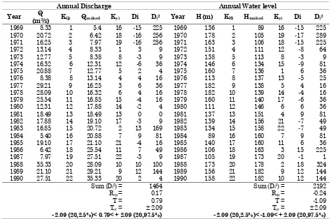
Table 3 show the results of the univariate analysis for annual water levels and annual discharges.
From the results, it can be deducted that the catchment discharge is unstable. The different behavior of discharges and levels imply that the developed relationship between the level and discharge may not be very reliable.
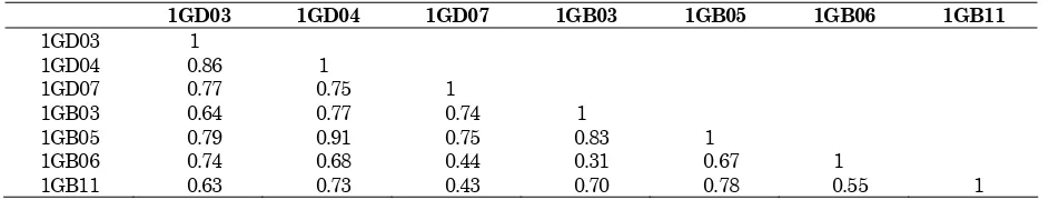
Bivariante description. Bivariante tools are used to describe relationship between two different variables or stations as shown in Tables 4 and 5.
The results in table show that the correlation between the annual discharges is less than the annual water levels. Therefore, filling in the missing data of the levels should be applied.
Behavioural trend, consistency and homoge-neity tests
The time series data provided (from gauging station 1GDO3) was analysed for behavioural trend, consistency, and homogeneity tests. Spearman’s t
test was applied for behavioural trend, F-test and Students t-test for consistencies in basic statistical parameters of mean and variance [7].
Spearman’s rank correlation.The basic principle was to rank the annual (monthly) values, Xi in ascending order of magnitude, denoted as ri, the rank one being r1. For a given Xi, (ri-i) was computed in which the statistics Rsp was subsequently generated. Thus, the expression is;
Rsp=
∑
= −
−
− n
i
i i
r n
n 1
2
2 ( )
) 1 (
6
1 (5)
To test whether there was presence or absence of trend, the student statistics t was computed, where;
t =
2
1
2
sp
R
n
Rsp
−
−
(6)Table 3. Univariate analysis for the annual water level (cm) and annual discharges
the annual water level (cm) the annual discharges (m3/s) Station
Mean S Cv β Mean S Cv β
1GD03 144 26.2 0.18 -0.39 17.64 8.07 0.46 0.37
1GD04 44 15.3 0.35 -0.19 14.83 6.11 0.41 -0.05
1GD07 257 12.4 0.05 0.40 7.52 4.48 0.60 1.24
1GB03 64 15.8 0.25 0.36 5.98 3.27 0.55 1.07 1GB05 83 14.2 0.17 0.04 3.74 1.91 0.51 0.59 1GB06 44 12.0 0.27 -0.90 1.22 0.55 0.45 -0.11 1GB11 86 12.8 0.15 1.57 0.98 0.76 0.77 2.87
Table 4. Correlation coefficients of annual discharge between various stations
1GD03 1GD04 1GD07 1GB03 1GB05 1GB06 1GB11 1GD03 1
1GD04 0.86 1
1GD07 0.77 0.75 1
1GB03 0.64 0.77 0.74 1
1GB05 0.79 0.91 0.75 0.83 1
1GB06 0.74 0.68 0.44 0.31 0.67 1
1GB11 0.63 0.73 0.43 0.70 0.78 0.55 1
Table 5. Correlation coefficients of annual water levels between various stations
1GD03 1GD04 1GD07 1GB03 1GB05 1GB06 1GB11
1GD03 1
1GD04 0.94 1
1GD07 0.83 0.87 1
1GB03 0.79 0.80 0.64 1
1GB05 0.78 0.84 0.75 0.62 1
1GB06 0.80 0.76 0.60 0.60 0.67 1
and compared against the tabulated Students t-distribution values with α/2 confidence level and n-2 degrees of freedom using two tailed test, (Table 6).
From the results of Spearmen`s test, it can be concluded that both discharges and levels at the gauging station 1GDO3 has developed some form of trend.
F and t tests
F test,
The data was further divided into two non-overlapping subsets to test for consistency (stability) of the mean and the variance. The non-overlapping subsets were denoted as j=1,2,---,m for subset 1, and j=m+1, m+2,---,n for subset 2. The respective mean and variance of the two subsets were than determined. The variance of the two subsets were examined using the F-test, in which the test statistics is
F =
The t-test was applied to the means to determine whether the two sets of data were significantly different from each other. The formulation used was
t = tabulated value with α/2 significance level, with m-1 and n-m-1 degrees of freedom. The results obtained are presented in Tables 7 and 8 In this case α is taken as 0.05.
Table 7. Statistics of the sub-sets of annual discharge and level data for 1GDO3
Mean Deviation Standard Years Number
Table 8. Results from split-record testing Computed value for Test
statistic Discharge level
Tabulated value for
F 0.66 0.68 3.72
T 0.29 2.32 2.09
Since the calculated F and t applied to the variances and means of the sub-sets of annual flow laid within Table 6. Trend test for annual discharges and levels (1GDO3)
Annual Discharge Annual Water level
the boundaries of the distributions, it was concluded that the variance of the two subsets were stable, hence came from a stable population without variation. The discharge data from 1GDO3 were therefore considered satisfactory for further analysis. The result of the t test applied to means of the levels showed that calculated t value was higher than tabulated value. From this it was proposed that the bed of the river is changing with time, and updating of the rating curve for further detail study of the area was recommended for verification.
Extreme Flow Analysis
The annual monthly discharges for the target station 1GD03 were visually inspected for extreme events and peaks over a certain threshold. For flood events it is practical to deal with instantaneous peaks where all flood events are conserved. Converting to monthly values often smoothen out peaks by averaging effects, thus significant food events are truncated.
Comparisons were made, by applying different but commonly available frequency distributions. They include the Gumbel, log normal, log-Pearson III, and Pearson III. During the study it was found that although log-Pearson III and Pearson III distri-butions described the peak sample distribution adequately, the sample population selected did not represent the annual events (peaks over threshold used). Therefore, Gumble was the qualified choice of distribution for the flood frequency analysis.
The Gumble distribution emanates from a family of General Extreme Value (GEV) distribution. In its original form Gumble is commonly referred to as Extreme Value Type I distribution (EV1) [6].
Theory of EVI distribution
The Cumulative Distribution Function (CDF) of EV1 (Gumble) is expressed as:
⎥
Expressing the CDF in terms of the Probability Density Function (PDF) yields the following:
⎥
where a is the scale parameter and c the location parameter and shape factor being zero.
The parameters are related to the sample mean (µ) and variance (σ) through the given relationship:
a Method of Moments (MOM), Maximum Likelihood (ML), Least Squares (LS), and Probability Weighted Moments (PWM). The skewness of EV1 is estimated as 1.14, while the standardised variant is given by the formulation:
Expressing G(yi) in terms of recurrence intervals and inverting the equation, the following equation for standard yi variate is derived.
⎥⎦
where T is given in years. Because the annual series is applied, any event with a recurrence interval of T
has a probability 1/T of being exceeded in any given year. The probability of non-exceedence of any given flood event is thus given as
The graphical fitting is a simple method using Fi as the plotting positions. Fi is expressed as;
α population and α =0.44, the Gringorten plotting position for EV1. Considering Equation 17, Equation 16 can be reduced to
[
i]
i F
y =−ln−ln (19)
Hence, the quantile can be conveniently estimated from the following relationship,
Xi=c+ ayi (20)
All estimates of quantiles have some inherent errors regardless the form of distribution applied. This may be attributed to sample errors, inappropriate distribution or inadequacies in parameter esti-mation. It is therefore advisable to test for goodness of fit for a given distribution by estimating quantile standard errors. For a two parameter EV1 distri-bution with T year recurrence interval with its estimate XT, the standard error of the estimate SE
can be expressed as:
and y is the standardised variate. Hence, the 95% confidence limits can be obtained as:
SE t X
CL= T ± 97.5,n−1 , (23)
where
t
97.5,n−1 is the value of two tailed (5%) t-distribution for 97.5% confidence limit with n-1 degrees of freedom [6].
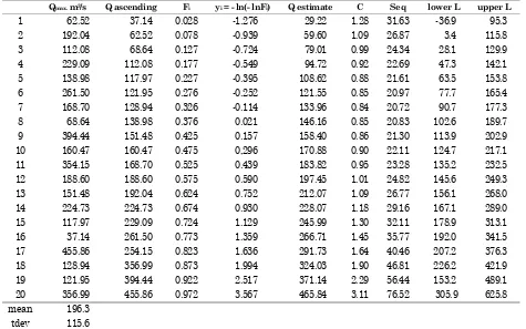
Table 9. Frequency analysis using Gumbel distribution
Qmax. m3/s Q ascending Fi yi = - ln(- lnFi) Q estimate C Seq lower L upper L
1 62.52 37.14 0.028 -1.276 29.22 1.28 31.63 -36.9 95.3
2 192.04 62.52 0.078 -0.939 59.60 1.09 26.87 3.4 115.8
3 112.08 68.64 0.127 -0.724 79.01 0.99 24.34 28.1 129.9
4 229.09 112.08 0.177 -0.549 94.72 0.92 22.69 47.3 142.1
5 138.98 117.97 0.227 -0.395 108.62 0.88 21.61 63.5 153.8
6 261.50 121.95 0.276 -0.252 121.55 0.85 20.97 77.7 165.4
7 168.70 128.94 0.326 -0.114 133.96 0.84 20.72 90.7 177.3
8 68.64 138.98 0.376 0.021 146.16 0.85 20.83 102.6 189.7
9 394.44 151.48 0.425 0.157 158.40 0.86 21.30 113.9 202.9
10 160.47 160.47 0.475 0,296 170.88 0.90 22.11 124.7 217.1
11 354.15 168.70 0.525 0.439 183.82 0.95 23.28 135.2 232.5
12 188.60 188.60 0.575 0.590 197.45 1.01 24.82 145.6 249.3
13 151.48 192.04 0.624 0.752 212.07 1.09 26.77 156.1 268.0
14 224.73 224.73 0.674 0.930 228.07 1.18 29.16 167.1 289.0
15 117.97 229.09 0.724 1.129 245.99 1.30 32.11 178.9 313.1
16 37.14 261.50 0.773 1.359 266.71 1.45 35.77 192.0 341.5
17 455.86 254.15 0.823 1.636 291.73 1.64 40.46 207.2 376.3
18 128.94 356.99 0.873 1.994 324.03 1.90 46.81 226.2 421.9
19 121.95 394.44 0.922 2.517 371.14 2.29 56.44 153.2 489.1
20 356.99 455.86 0.972 3.567 465.84 3.11 76.52 305.9 625.8
mean 196.3 tdev 115.6 Skew 0.87
Var 13354.8 a 90.15 c 144.23
0.0 100.0 200.0 300.0 400.0 500.0 600.0 700.0
-2.0 -1.0 0.0 1.0 2.0 3.0 4.0
standardised variate
annual
m
ax
.
di
s
c
har
ge,
m
3 /
s
observed
computed
The results of flood frequency analysis are shown in Table 9 and Figure 3.
Observed data are within 95% confidence limits and data can be represented by the Gumbel distribution. Thus the 5, 10 and 20-year design floods are 279m3/s, 347m3/s, and 439m3/s respectively.
Results and Discussion
Four flood mitigation structures; flood plain exten-sion, embankment (dykes), channel by-pass, and green-storage were simulated for 20-year recurrence interval flood to determine their individual responses in storing excess water.
If the water depth at Ahero exceeds 5m, the area downstream will be flooded. Analysis for the base-case and all other flood mitigation schemes was carried out for the 14-22 April 1988 flood period, taken also as the 20-year recurrence interval flood
(design flood). For the base-case at Ahero’s bridge (node 1), water depth was 10.9m, and at 10km downstream Ahero (node 3), the water depth was 6.0m. Water depths were then compared against the base-case by running the proposed mitigation schemes:
• Flood plain result showed that the water depth at node 1 and 3 was 4.8 m and 4.2 m respectively. This means that Kano plain has a better chance of not being flooded with maximum discharge equalling 434.173 m3/s (modelled).
• By constructing embankment (dykes) the water depth at node 1 increased to 10.6 m and at node 3 to 3 m. The result therefore suggests that the nominal height of the dykes to be constructed is 5.6 m, while water depth at downstream is further reduced.
• Channel by-pass result showed that the water depth would be below 5 m with a diversion located 8.28 km downstream of Ahero. The width of the diversion in this simulation was 25 m.
0 2 4 6 8 10 12 14
15-Apr-88 16-Apr-88 17-Apr-88 18-Apr-88 19-Apr-88 20-Apr-88 21-Apr-88 22-Apr-88
D
e
pt
h (
m
)
Base-case Dykes Floodplain Bypass Original green
Dykes
Base-case
Original green
By-pass
Flood-plain
Figure 4. Comparison of water depth at Ahero (node 1)
0 1 2 3 4 5 6
15-Apr-88 16-Apr-88 17-Apr-88 18-Apr-88 19-Apr-88 20-Apr-88 21-Apr-88 22-Apr-88
De
p
th
(m
)
Dykes Floodplain Bypass Base case Original green
Dykes
Original green Base-case
By-pass
Flood-plain
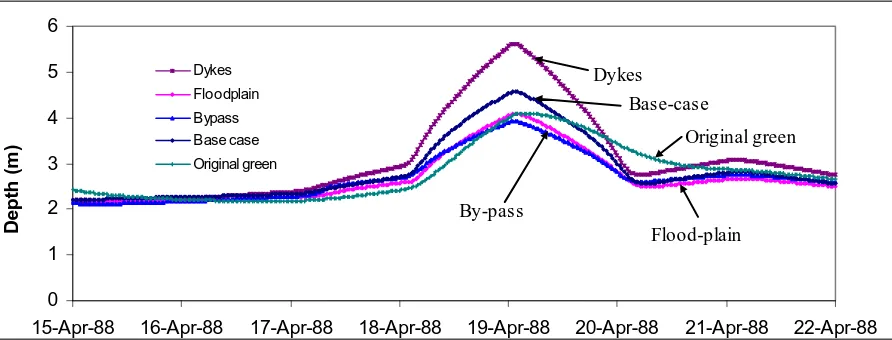
• Green-storage result showed that the water depth was 9.8 m and 4 m at node 1 and 3 respectively. In this situation, the upstream will continue experience flooding, but downstream not flooded in any form
From Figures 4 and 5, it can be seen that the water depth of downstream nodes are higher than that of upstream nodes. It is mainly because that the river bed slope along the channel is not the same, the bed slope of first section is 0.001 m/m, and others are 0.00055 m/m, according to Manning formula, the velocity of section 2 to section 5 is less than that of section 1, so the water depth increased in node 3.
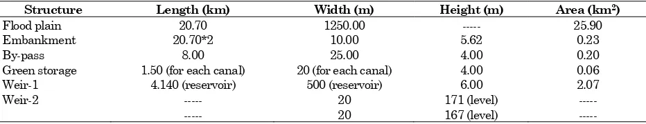
Dimensions of flood mitigation measures. For 20-year recurrence interval flood, the size and anticipated occupied area of every structure are shown in Table 10.
Social Economical And Environmental Issues. During peak flow periods, the industries, the fertile agricultural lands, and villages are inundated with floodwaters. Consequently, this causes loss of life and damage to property, transportation, and tele-communication systems disrupted. The economic and social activities are further influenced seriously. Hence, in order to mitigate or minimise the flood disaster, appropriate flood control structures needed to be constructed in the downstream of Ahero.
When there is no structure for flood mitigation (base case), disastrous floods cause loss of life and property damage, with high monetary costs. It is expensive in term of finance and other resources (labour and machinery) to clean up the debris, and to restore the damaged structures. Opting for flood mitigation structures, on the other hand attenuates peaks propagating downstream but magnitudes vary, depending on which mitigating scheme is used. Disadvantages. The initial costs of mitigation schemes may not only be expensive. Impacts to social and environment aspects needed to be considered when recommending a scheme. Some notable inclusions for flood-plain extension, channel by-pass and green storage are;
• Reduction of the size of arable and grazing land, • Diversifying the useable land,
• Developing resettlement schemes for displaced local people, and
• Depriving people of their rights to use the land in whatever forms that is beneficial.
Furthermore, if the water in the green-storage and flood plain extension is not drained out in adequate time it has the potential of breeding mosquito (since tropical area), which will pose health hazard to the people.
Constructing embankments (dykes) should not be a viable option since its linear extension is unpredic-table, hydraulic components not accounted for (backwater curve, foundation strength, risks of failure), and material required for construction is seemingly dear.
Advantages. Channel by-pass may serve as a shortcut navigation route to reach Ahero. Green-storage will always maintain certain amount of water, which in turn can be used for recreation, fishing, other water sports, and maintenance of the environment.
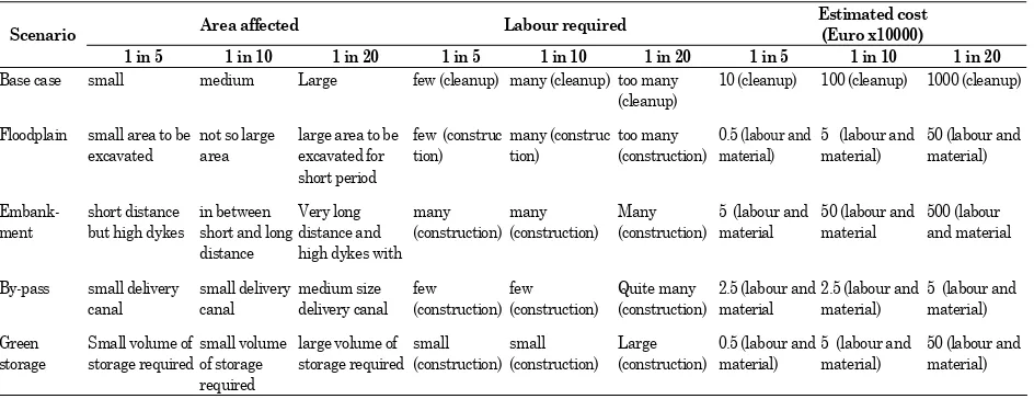
The scoreboard, as shown in Table 11, provides an overview of the conditions to be expected in real life (practical) situations when such extreme events do occur. Not only the population living downstream of Ahero and the Kano flood plain will be affected, but the environment, fauna and flora, the local, district and the national administrators, and the parties that influence the local economy.
Conclusion
The following conclusions were made from the study results:
• Average discharge is 17.6 m3/s at the outlet station 1GDO3, the relationship between the level and discharge is not very reliable. Because the bed of the Nyando river is changing with time (specially after high floods).
• The Gumbel distribution was accepted to be a good fit and this distribution was used for the flood frequency analysis. Design floods with return period 5, 10, 20 years are 279 m3/s, 347 m3/s, and 439 m3/s respectively.
Table 10. Scheme dimensions
Structure Length (km) Width (m) Height (m) Area (km2)
Flood plain 20.70 1250.00 --- 25.90
Embankment 20.70*2 10.00 5.62 0.23
By-pass 8.00 25.00 4.00 0.20
Green storage Weir-1 Weir-2
1.50 (for each canal) 4.140 (reservoir)
--- ---
20 (for each canal) 500 (reservoir)
20 20
4.00 6.00 171 (level) 167 (level)
• Various design flows are simulated against the different structures, such as dyke/embankment, green storage, channel-bypass, and flood plain-extension. Flood plain-extention are fairly well known , however, topographical details were not available. Hence the optimal structure suggested is green-storage.
Recommendation
It is recommended that:
• Flood data for every year should be checked in future study.
• The rating curves should be updated after high floods. This include updating of the river cross-section
References
1. Spaans, W., Groupwork Nyando Catchment,
Notes,IHE,The Netherlands, 2003.
2. Wanjohi, D. M., Water Flow and Quality
Modelling of the Nyando River in Kenya,Thesis,
IHE,The Netherlands, 1999.
3. Njogu, A. K., An Intergrated River Basin Planning Approach–Nyando Case Study in Kenya, M.Sc.Thesis, IHE,The Netherlands, 2000.
4. Agha, H. U., Surface Water in the Nyando Catch-ment, Individual study, IHE, Delft, The Nether-lands, 2000.
5. Duflow Modelling Studio, User’s Guides, Stowa, EDS, 2000.
6. Hall, M. J., Statistic and Stochastic Processes in
Hydrology, Lecturer Notes, IHE, The
Nether-lands, 2003.
7. De Laat, P. J. M., Workshop on Hydrology, Lec-turer Notes, IHE, The Netherlands, 2001. Table 11. Scoreboard for the 1 in 5, 1in 10 and 1 in 20 year design floods
Area affected Labour required Estimated cost (Euro x10000) Scenario
1 in 5 1 in 10 1 in 20 1 in 5 1 in 10 1 in 20 1 in 5 1 in 10 1 in 20 Base case small medium Large few (cleanup) many (cleanup) too many
(cleanup)
10 (cleanup) 100 (cleanup) 1000 (cleanup)
Floodplain small area to be excavated but high dykes
in between short and long distance
By-pass small delivery canal
Small volume of storage required
small volume of storage required
![Figure 1. Nyando catchment relief pattern [1]](https://thumb-ap.123doks.com/thumbv2/123dok/3649733.1465363/2.595.72.538.81.419/figure-nyando-catchment-relief-pattern.webp)