JEJAK
Journal of Economics and Policy http://journal.unnes.ac.id/nju/index.php/jejak
Mundell-Fleming Model: The Effectiveness of
Indonesia’s Fiscal
and Monetary Policies
Nurjannah Rahayu K1 , Phany Ineke Putri2
Semarang State University
Permalink/DOI: http://dx.doi.org/10.15294/jejak.v10i1.9137
Received: April 2016; Accepted: July 2016; Published: March 2017
Abstract
This study examines the fiscal and monetary policy in Indonesia using the Mundell-Fleming model. The main objective of this study was to determine which policies are effective between fiscal and monetary policies of the national income in Indonesia because Indonesia is a small open economy with not perfect capital mobility. The analysis technique used is Two Stage Least Square (TSLS) by using secondary data base on International Financial Statistics, 2000.I – 2014.II . The research result is monetary policy is more effective than the fiscal policy in which monetary policy multiplier at 0.0028 greater than fiscal policy multiplier 0.001316. The results are consistent with the theory of the Mundell-Fleming.
Key words : Mundell Fleming, Efectivity, Monetary Policy, Fiscal Policy.
How to Cite: K, N., & Putri, P. (2017). Mundell-Fleming Model: The Effectiveness of Indonesia’s Fiscal and Monetary Policies. JEJAK: Jurnal Ekonomi Dan Kebijakan, 10(1), 223-235. doi:http://dx.doi.org/10.15294/jejak.v10i1.9137
© 2017 Semarang State University. All rights reserved
Corresponding author :
Address: Campus Sekaran Gunungpati Semarang 50229 E-mail: [email protected]
INTRODUCTION
The issued policy can be fiscal policy and monetary policy. Besides, by observing the financial crisis that rapidly spreads and defeats the monetary sector, monetary policy may be more effective than fiscal policy. This is in line with the opinion of Mundell and
Fleming. Mundell-Fleming’s theory is to
study and analyze economic phenomena, there is a need to use any models. Therefore, Macro-economic model which can be used to analyze the fiscal and monetary policies which work in an open economy is Mundell Fleming model. The model is also called the IS-LM-BP (Makin, 2002). It explains short
fluctuation in GDP, exchange rate,
consumption, investment, government
spending, net exports and enters
international capital flows.
Yarbrough and Yarbrough (2002) state that the exchange rate system adopted and the degree of international capital flows are the determinant of the effectiveness of monetary and fiscal policy in open economies. The differences of exchange rate system used in the economy will greatly influence the effectiveness of economic policy and the determination of the exchange rate.
Mundell-Fleming’s theory is intended to study and analyze economic phenomena, where a model is needed. Macro-economic model is to analyze fiscal and monetary policies. Mundell-Fleming explains short-term fluctuation in Gross Domestic Product, exchange rate, consumption, investment, government expenditure, and net export and includes international capital flow.
Mundell-Fleming suggests that monetary policy is more effective compared to fiscal policy to increase GDP. This Mundell-Fleming’s finding could work
because it is built on an assumption that there is a perfect capital flow as a result of the absence of difference between domestic and foreign interest rates.
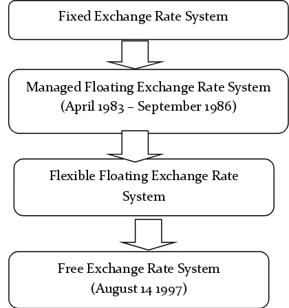
Mundell-Fleming model showed that the effects of any economic policies in a "small open economy" depend on the regime or system of exchange rates which were followed by the economy, it can be fixed exchange rate regime or flexible exchange rate regime. In other words, the effectiveness of fiscal and monetary policy in influencing the aggregate income depends on the exchange rate regime. Under the floating or flexible exchange rate regime, there only lies the effective monetary policy which. It means that it can affect the income. Oppositely, under the fixed exchange rate regime, there is only fiscal policy which can affect income.
Mundell-Fleming states that monetary policy is more effective to improve GDP than fiscal policy. Mundell-Fleming's finding can run because it is built on an assumption by the existence of perfect of flow capital as a result of no differences of domestic interest rates and abroad interest rates (Mankiw, 2000: 291).
Mundell-Fleming states that monetary policy is more effective to improve GDP than fiscal policy. Mundell-Fleming's finding can run because it is built on an assumption by the existence of perfect of flow capital as a result of no differences of domestic interest rates and abroad interest rates (Mankiw, 2000: 291).
Source : Workshop of Indonesian Central Bank
Figure 1. Exchange Rate System History in Indonesia
As to the objectives, this study aims at: (1) Discovering and reviewing the simultaneous impacts of fiscal and monetary policies on GDP; (2) Discovering and reviewing the effectiveness of fiscal and monetary policies in increasing GDP.
RESEARCH METHODS
This study focuses on fiscal and
monetary policies towards Indonesia’s macro
economy during a period of 2000.I – 2014.II.
The data used in this research are secondary one obtained from International Financial Statistics, issued by International Monetary Fund (IMF), Bank Indonesia and BPS. The analysis model used is simultaneous regression analysis to determine the level of correlation and influence occurring with two-stage least square method.
The research model used is simultaneous equation model estimated using Two Stage Least Square (TSLS) method.
IS Equation Block
... (1.1)
... (1.2)
... (1.3)
... (1.4) ... (1.5)
... (1.6)
LM Equation Block
... (1.7)
... (1.8)
... (1.9)
Fixed Exchange Rate System
–
Managed Floating Exchange Rate System (April 1983 – September 1986)
Flexible Floating Exchange Rate System
(September 1986 – August 1997)
BOP Equation Block
𝐵𝑜𝑃𝑡 = 𝑗0 + 𝑗1𝐾𝑈𝑅𝑆𝑡+ 𝑗2𝐷𝐼𝐹𝐹𝑅𝑡
... (1.10)
IS Curve Equation Model
Based on each result of the equations previously done which form IS, the IS
equation could then be calculated as follows:
Yt = Ct + It + Gt + Xt + Mt
Yt = C0 + cYt + I0 – bIntt + G0 + X0– (M0 + mYt – zKurst)
Yt = C0 + cYt + I0 + G0 + X0– M0 – mYt + zKurst – bIntt
𝑌𝑡 = 1−𝑐+𝑚1 {𝐶0+ 𝐼0+ 𝐺0+ 𝑋0− 𝑀0+
𝑧𝐾𝑢𝑟𝑠} − 1−𝑐+𝑚𝑏 𝐼𝑛𝑡𝑡 (1.11)
From the equation above, it is found C, I, G and X multipliers are
1
1−𝑐+𝑚 (1.12)
As to M multiplier, it is −1
1 − 𝑐 + 𝑚 If ; 𝛼 = 1
1−𝑐+𝑚
A = C0 + I0 + G0 + X0– M0 + zKurst; that , Yt = α ( A – bInt)
In which:
Y : Gross Domestic Product; C : Total Consumption; I : Total Investment;
G : Total Government Expenditure asta; X : Total export;
M : Total import; Int : Interest Rate; Kurs : Exchange rate;
c : Coeffisien variable GDP at consumption equation;
b : Coeffisien variable interest rate at investment equation;
m : Coeffisien variable GDP at import equation;
z : Coeffisien variable exchange rate at import equation;
t : time
LM Curve Equation Model
Balancing Money market when Ms = Md, therefore the LM equation is:
Ms0 = Md0 + kYt – hIntt -kYt = Md0 – h Intt – Ms0
kYt = Ms0– Md0 + h Intt (1.13) if B=Ms0– Md0 that:
𝑌𝑡 =1𝑘(𝐵 + ℎ𝐼𝑛𝑡𝑡) (1.14)
𝐼𝑛𝑡𝑡=ℎ1(𝑘𝑌𝑡− 𝐵) (1.15)
In which:
Ms : Supply of money; Md : Demand of money;
k : Coeffisien variable GDP at demand of money equation;
h : Coeffisien variable interest rate at demand of money equation
Balance IS-LM
IS-LM balance that happen when IS curve crossed with LM curve, could then be
calculated as follows:
Yt = α ( A – bInt)
Intt = 1ℎ(𝑘𝑌𝑡− 𝐵)
𝑌𝑡 = 𝛼 [𝐴 − 𝑏ℎ (𝑘𝑌𝑡− 𝐵)]
𝑌𝑡 = ℎ+𝑘𝑏𝛼ℎ𝛼 𝐴 + ℎ+𝑘𝑏𝛼𝑏𝛼 𝐵
Fiscal Policy Multiplier
Monetary Policy Multiplier
Monetary policy multiplier shows to what extent the distributed number of real money can increase the equilibrium income level, without any fiscal policy change. In reference to equations 3.13 and 3.16, the Fiscal Monetary Multiplier (MKF) in Indonesia could then be calculated as follows:
(3.18)
RESULTS AND DISCUSSION
Fiscal policy
In fiscal policy, the main indicator is the State Budget (APBN) (Raharja and Manurung, 2001). During the budget of 1997/1998 the increase of government spending was higher 63% than the previous year. It was the government policy to affect economic growth by which, at that time, it was the early beginning of the economic crisis. The same thing happened in a different budget that was in 2002/2003 which reached 85% higher than the previous year.
The increase of government spending will increase economic activity, but the threat of instability in the economy in the form of threat of inflation is probably difficult to avoid. APBN which is regarded as the locomotive of economic growth is possible to cause it because it is done based on the belief that the government economic sector is needed for the implementation of trilogy development, namely: growth, equity, and stabilization. This trilogy is the realization of the theory of fiscal functions, namely the allocation of public goods
(allocation), income distribution
(distribution), and economic stabilization (stabilization).
The crisis that occurred in Indonesian economy in 1997 led the government to increase the spending. The cost of banking restructuring and real sector recovery had led the government to increase the budget deficit by considering that the limited resources funds owned. Alternatively, the budget deficit considerably increased after the 1997 crisis, especially in the period of state budget in 1999 which reached Rp 114585 billion. On the other hand, Bank Indonesia applied contractive monetary policy to fend off inflation and control the money supply. At that time, the recorded interest rate highly increased, that was about 25% in 1998 and an average of 22% in 1999.
On the other hand, appropriate fiscal policy does not give results as wished, because it is not only fiscal policy which can affect the economy of Indonesia, but also monetary policy which is controlled by the monetary authority. Fiscal and monetary policies in many cases often cause the opposite effect or crowding out. As a result, it becomes necessary to have good and appropriate coordination mechanism in order the goals of economic development that have been set can be achieved.
Monetary policy
Price and exchange rate stability are the requirement for economic recovery because the economic activity of society, the business sector, and the banking sector will be hampered without them. Therefore, it is reasonable if the main focus of Bank Indonesia monetary policy during this economic crisis is to achieve and maintain price stability and the exchange rate of rupiah.
the stability of exchange rate of rupiah in which there is an understanding of price stability and the stability of exchange rate of rupiah.
To achieve the above-mentioned objectives, recently, Bank Indonesia still applies the monetary policy framework which is based on controlling the money supply. Hence, Bank Indonesia has sought to control base money as the operational target of monetary policy.
With the controlled amount of base money, the growth in the money supply; M1 and M2, are also expected to control. Furthermore, with the controlled money supply, it is expected that the aggregate demand for goods and services are always moving in a balanced amount to the national production capabilities, so prices and exchange rate can move stably.
By using the monetary policy
framework as described above, Bank Indonesia in the early period of economic crisis, especially during 1998, applied a tight monetary policy to restore monetary stability. The tight monetary policy is reflected in the annual growth of the indicative target money supply which was continually pressed from the highest level of 30.13% in 2000 to 9.58% in 2001. The tight monetary policy has to be done because in that period of inflation expectations in society was very high and the money supply was rapidly increased.
During the high inflation expectations and the level of the risk of holding rupiah, the effort to slow the rate of growth of money supply have supported domestic interest rates sharply. Further, high interest rates are needed in order to make people
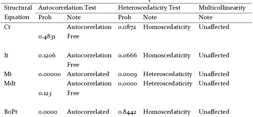
Prior to performing any regression, the model ought to be tested first against classic assumption deviation. Such testing is performed to obtain a BLUE estimator. The classic assumption tests which need to be done are autocorrelation, heteroscedasticity and multicollinearity tests.
For the heteroscedaticity, the test used is White Test. This White test is different from several other methods to test heteroscedaticity because it does not require any assumption about the existence of its residual normality (White, 1980 in Primastuti, 2008).
The autocorrelation test in this research uses LM test method. This test is capable of accommodating a non-stochastic independent variable in a regression model.
For its multicollineariety, this study uses auxiliary regression method where in performing the regression, all of its variables are interchangeably used as dependent variables.
Table 1.
Results of Assumption Tests
StructuralEquation
Autocorrelation Test Heteroscedaticity Test Multicollinearity
Prob Note Prob Note Note
Ct
0.4831
Autocorrelation Free
0.0872 Homoscedaticity Unaffected
It 0.1206 Autocorrelation Free
0.0666 Homoscedaticity Unaffected
Mt 0.00000 Autocorrelated 0.0009 Heteroscedaticity Unaffected Mdt
0.123
Autocorrelation Free
0,0000 Heteroscedaticity Unaffected
BoPt 0.0000 Autocorrelated 0.8442 Homoscedaticity Unaffected
Equation Analysis
a)
Consumption EquationHerewith the result of the Consumption equation analysis, below:
CT = 36.398,3720032 + 0,521745369338*YT – 0,0665073320915*T0
(4,799) (21,185) (-1,849)
R2 = 0,99 Fstat = 21680,83
The Yt coefficient at 0.52 means that the Marginal Propensity to Consume (MPC) was at 52%. This figure is quite relevant to the developing countries like Indonesia that more than half of their income are used for consumption. The results of this study are in line with research conducted by Noor Cholish (2007) amounted to (62%), Abbullah Suparman (1990) that the MPC of his research results was at 47% and research results of Teguh Santoso’s (2009) by 54%.
In this study, tax affects national income at the level of α = 10%. It means that the tax increase will reduce consumption. The higher the taxes that are imposed by the government will decrease the amount of its disposable income and also will reduce the
amount of consumption goods and services.
Based on the regression equation results, C score can be calculated as follows:
Ct = c0 + c1 (Yt – T0)
Ct = 36.398,37 + 0,52Y – 0,066 (T0)
Ct = 36.398,37 + 0,52Y – 0,066 (118.262,98) Ct = 28.593,02 + 0,52Y
b)
Investment EquationHerewith the result of the investment regression equation, below:
IT = -27.097,0338064 – 445,963982543*RT + 0,302072587841*YT
(-3,658) (-1,084) (23,993)
R2 = 0,96 Fstat = 872,0166
consider the interest rate but also the condition of macro-economic overall.
Meanhile, the variable of national income (Yt) gave positive effect on investment in the level of α = 10%. This result is in accordance with the theory of Keynes that the national income has positive effect on investment. Moreover, the higher someone’s income, so the investment which has done does. Again, for some people, investment is a form of precaution and speculation to get profit at once.
Based on the regression equation results, I score can be calculated as follows:
It = I0 – b1Rt + b2Yt
It = -27.097,03 – 445,96Rt + 0,30Yt
c)
Government Expenditure EquationThe government expenditurescore is taken from the mean government expenditurefrom 1998 quarter I through 2014 quarter II, i.e. amounting to Rp 36.782,08
Gt = G0 = 36.782,08
d)
Export EquationThe export score is taken from the mean export from 1998 quarter I through 2014 quarter II, i.e. amounting to Rp 214.466,09
Xt = X0 = 214.466,09
e)
Import EquationHerewith the result of the import regression equation, below:
MT = -138.796,591431 + 0,414313810628*YT + 11,4999942982*KURST
(-2,917) (16,141) (1,983)
R2 = 0,88
Fstat = 260,0787
If the national income increases, the tendency for importing is high. The increase income means having ability to buy imported goods which is much greater than the assumption of other factors, and is deemed to be constant.
Variable of exchange rate which affects to imports isnot in accordance with the theory. It is because of most of industries in Indonesia use imported raw materials. It is confirmed by BPS data about the import goods according to the category of use (Figure 4.8). Figure 4.8 shows that the imports which are carried out by Indonesia are mostly in the form of raw materials and auxiliary goods industry.
Based on the regression equation results, M score can be calculated as follows:
Mt = m0 + m1Yt – m2 Kurst
= -138.796,6 + 0,41Yt + 11,49Kurst
IS Equation
Based on each result of the equations previously done which form IS, the IS equation could then be calculated as follows:
Yt = Ct + It + Gt + Xt - Mt
Yt = 28.593,02 + 0,52Yt + (-27.097,03 – 445,96Rt + 0,30Yt) + 36.782,08 + 214.466,09 – (–138.796,6 + 0,41Yt + 11,49Kurst)
Y = 663.628,41 – 19,47Kurst – 755,86Rt
From the equation above, it is found C, I, G and X multipliers are
=
Source : Central Statistic Bureau, processed.
Figure 2. Import by the goods categorizing by 1998-2014 (Million Dollar).
Transformation of Equation of LM Equation Block
a)Money Supply Equation
The money supply score is taken from the mean money demand from 1998 quarter I through 2014 quarter II, i.e. amounting to Rp 1,600,956.64
Mst = Ms0
Mst = Ms0 = 1.600.956,64
b)
Money Demand EquationHerewith the resukt of money demand regreesion equation, below:
MD = -482.938,421178 + 1,80301731909*YT
– 344,491969992*RT
(-8,447) (18,988) (-0,256)
R2 = 0,89 Fstat = 263,9367
When the income increases then the demand for money also increases. This is in accordance with the theory of JM.Keynes that the demand of money is influenced by the level of income. The higher income level,
the transaction motive and precaution have also increased and led to the increasing demand of money.
Variable of interest rate did not affect the demand of money. The results of this study reject the hypothesis Keynes. The results of this study was caused by the Indonesian society which are middle class society that their monetarization level is not quite high and some of their money are for consumption.
As to the money demand equation, it is as follows:
Mdt = Md0 + hYt – kRt
Mdt = –482.938,4 + 1,80Yt -344,49Rt
LM Equation
Based on each result of the equations previously done which form LM, the LM equation could then be calculated as follows:
Ms = Md
1.600.956,64 = –482.938,4 + 1,80Yt – 344,49Rt Yt = 1.157.719,46 + 191,38Rt
Transformation of Payment Balance Equation
BOP = -32.388,42115 + 3,26870017861*KURST + 26,1053327272*DIFFRT
(-4,039) (3,814) (0,443)
R2 = -0,35 Fstat = 7,678051
The T-test for the variable of exchange rate gave positive effect and had significant at α = 5% toward the balance of payments. Besides, the differentiation variable of SBI interest rate and Libor had no effect on the balance of payments. Even though the differentiation in interest rates did not affect the balance of payments, according to the sign test it was already accordance with the theory.
If the value of the rupiah towards the US dollar decreased, the prices of domestic goods according to abroad consumers are cheaper than the current exchange rate when it is appreciated. Abroad consumers will increase the amount of consumption of goods and services produced by Indonesia. Therefore, exports will increase and the balance of payments will be surplus, assuming ceteris paribus.
The differentiation variable of interest rate did not affect the balance of payments since foreign people do not only consider the interest rate given by Indonesia when they want to invest their funds in Indonesia, but the factor of political stability and security are also considered.
As to the score of payment balance, it is as follows:
BOP = j0 + j1Kurst + j2diffrt
BOP = –32.388,54 +3,27Kurst + 26,10diffrt Kurst = 9.904,75 – 7,98 (9,44)
Kurst = 9.829,42
IS-LM Balance
Based on the IS and LM equations, the goods market and money market balance, i.e. national income and interest rate, could then be calculated as follows:
IS = LM Y = Y
663.628,41 – 19,47Kurst – 755,86Rt = 1.157.719,46 + 191,38Rt -947,24Rt = 494.091,05 + 19,47
(9.829,42)
Rt = –723,65
Y = 663.628,41 – 19,47Kurst – 755,86Rt Y = 663.628,41 – 19,47 (9.829,42) – 755,86 (-723,65)
Y = 1.019.227,69
Fiscal Policy Multiplier
Based on the research results, the amount of fiscal policy multiplier (MKF) could be calculated as follows:
MKF =
=
=
= 0,001316
This 0.001316 means that if the government expenditureis added with one unit, the national income will increase at 0.001316
times the sum of government
expenditureassuming that there is no change to the monetary policy.
Monetary Policy Multiplier
Based on the research results, the amount of monetary policy multiplier (MKM) could be calculated as follows:
MKM =
=
This 0.0028 means that if the distributed number of money is added with one unit, the national income will increase at 0.0028 times the sum of distributed number of money assuming that there is no change to the fiscal policy.
The Effectiveness of Policy Analysis
The monetary policy multiplier (0.0028) is greater than the fiscal policy multiplier (0.001316), hence, the monetary policy is more effective in influencing the
effective in influencing Indonesia’s economic
growth than the fiscal policy.
The fact that monetary policy is more effective as compared to the fiscal one confirms Mundell-Fleming’s theory. This Mundell-Fleming’s theory is that an open, small economy with floating exchange rate system is more effective to use monetary policy than fiscal policy. Indonesia is a small, open country with floating exchange rate system, thus, the results of this research confirm Mundell-Fleming’s findings.
Research on the effectiveness of fiscal and monetary policies in another country finds that monetary policy is more effective. Noor Cholish, using simple IS-LM model and ECM analysis technique, finds that monetary policy is more effective compared to fiscal policy. The fiscal policy multiplier is 0.6 and the monetary policy multiplier is 2.6.
Similar research is also conducted by Teguh Santoso. Teguh Santoso's research results confirm Mundell-Fleming’shypothesis
that monetary policy is more effective than fiscal policy. This can be seen from how significant the money demand variable is to
national income at α=5%, while the government
expenditureis significant at α=10%.
Another study is conducted by Barro (1991).He uses a number of modelswith different combined variables and simple regression analysis and cross sectiondata covering 98 countries for his observation during 1960-1985. He suggests that the government consumption expenditure (fiscal policy) has negative impact on both economic and investment growths. Using St. Louis model and making the United States his research site, Andersen and Carlson (1970), Carlson (1978), Hafer (1982), Dewald and Marchon (1978) in Triyono and Yuni Prihadi Utomo (2004) states that monetary policy is more dominant compared to fiscal policy instrument. Likewise, the research conducted to Canada, West Germany, France, Italy, Japan and England shows a result which place monetary policy as more determinant over economic growth than fiscal policy instrument.
Despite its results which indicate that monetary policy is more effective than fiscal policy in influencing national income increase, a little bit closer look at the calculation results of
each policy’s multipliers, either monetary policy
(0.0028) or fiscal policy (0.001316), would show that the difference of such multipliers is not that great. This is because in the case of this research, which takes the period of 1998 quarter I through 2014 quarter II, the policies taken by the Government could not be separated from the expansive fiscal policies. During that period, several economic phenomena occurred which
influenced Indonesia’s economy.
Rp 12,252.1 per United States Dollar in quarter III of 1998.The efforts made by BI to save the economy was to change the exchange rate system into the free, floating one, increasing BI rate. On one hand, the Government through the Department of Finance increased its expenditure in order to
drive Indonesia’s economy to a more stable
direction. These policies were contradictory, i.e. expansive fiscal policy and contractive monetary policy. It was then unsurprising that a crowding out occurred in 1998.
In 2005 the Government reduced fuel and oil subsidy, then in 2008 when a global crisis took place, the Government contributed to it through its fiscal stimulus. Therefore, it is just predictable that the difference between fiscal and monetary multipliersis not that great because the Government as the fiscal authority is fairly active in maintaining the economy. However, it is important to prevent the fiscal and monetary policies from conflicting one another. When the fiscal and monetary policies are contradictory, Indonesia’s macroeconomic objective could then never be realized.
CONCLUSION
Based on the research objective and data analysis, it could then be concluded as follows: monetary policy is more effective than fiscal policy. It can be seen from the monetary policy multiplier at 0.0028% where it is higher than the fiscal policy multiplier at 0.001316% and confirmed by the fact that the quantity level slope of IS curve model is elastic and the LM curve inclination level is less elastic. The research results confirm Mundell-Fleming’s theory which states that for an open, small economy with floating exchange rate system, it is more effective to use monetary policy than fiscal policy.
REFERENCES
Darwanto. (2007). ”Kejutan Pertumbuhan Nilai Tukar Riil
terhadap Inflasi, Pertumbuhan Output, dan Pertumbuhan Neraca Transaksi Berjalan di
Indonesia”. Jurnal Ekonomi Pembangunan Vol. 12 No.1, April 2007 Hal: 15 – 25
Dornbush, Rudiger. (1990). Makroekonomi. Jakarta : PT. Media Global Edukasi.
Frenkel, Michael,Isabell Koske. (2004). “How Well Can Monetary Factors Explain the Exchange Rate of The
Euro?” AEJ: September 2004, Vol. 32, No. 3
Gujarati, Damodar. (2001). Ekonometrika Dasar. Jakarta: Erlangga.
Husman, Jardine A. (2007). “Dampak Fluktuasi Nilai Tukar Terhadap Output dan Harga: Perbandingan
Dua Rezim Nilai Tukar”. Bulletin Ekonomi Moneter dan Perbankan, Juli 2007.
Hsing, YU, dan WEN-JEN Hsieh. (2005). “Impacts of Monetary, Fiscal and Exchange Rate olicies on
Output in China: A Var Approach”. Economics of Planning (2004) 37: 125-139, Springer 2005
Insukindro. (1993). Ekonomi Uang dan Bank : Teori dan Pengalaman di Indonesia. Yogyakarta : BPFE. Kuncoro, Mudrajad. (2001). Manajemen Keuangan
Internasional Pengantar Ekonomi dan Bisnis Global, Edisi Kedua. Yogyakarta : BPFE.
Kuncoro, Mudrajad. (2007). Metode Kuantitatif Teori dan Bisnis Aplikasi Untuk Bisnis dan Ekonomi. Yogyakarta : UPP STIM YKPN.
Krugman, Paul dan Obsfeld Maurice. (1992). Ekonomi Internasional. Jakarta : Rajawali Press.
Madura, Jeff. (2006). Keuangan Perusahaan Internasional, Edisi 8. Jakarta: Salemba Empat.
Madjid, Noor Cholis. (2007). Analisis Efektivitas Antara Kebijakan Fiskal dan Kebijakan Moneter dengan Pendekatan Model IS-LM (Studi Kasus Indonesia Tahun 1970-2005. Tesis, MIESP Universitas Diponegoro.
Mankiw, Gregory. (2000). Teori Makroekonomi Edisi 4. Jakarta : Erlangga.
Mishkin, Frederic. (2001). The Economics of Money, Banking and Financial Markets. Addison Wesley.
Ortiz, Javier, dan Carlos Rodriguez. “ Country Risk and The Mundell-Fleming Model Applied To The 1999-2000 Argentine Experience”. Journal of Applied Economics, Vol. V, No. 2 (Nov 2002), 327-348. Prasetyo, P.Eko. (2009). Fundamental Makro Ekonomi.
Yogyakarta : Beta Offset.
Pyndick, Robert., Daniel,Rubinfeld. (1991). Econometric Models and Economic Forecasts. New York: McGraw Hill.
Saeed, Ahmed, dkk. (2012). “An Econometric Analysis of
International Journal of Business and Social Science Vol. 3 No.6 (Special Issue-March 2012) Santoso, Teguh, dan Maruto Umar Basuki. (2009).
“Dampak Kebijakan Fiskal dan Moneter dalam Perekonomian Indonesia: Aplikasi Model Mundell-Fleming”. Jurnal Organisasi dan Manajemen, Volume 5, Nomor 2, September 2009, 108-128
Saptutyningsih, Endah. (2006). “Analisis Pengaruh
Kurs terhadap Kondisi Makro Ekonomi Indonesia Dari Sisi Permintaan Pendekatan
Persamaan Simultan”. Media Ekonomi Vol.12 No.3 Desember 2006
Shahbaz, Muhammad, dkk. (2011). “The Exchange Rate of The Pakistan Rupee and Pakistan Trade
Balance : An ARDL Bounds Testing Approach”.
The Journal of Developing Areas Volume 44, Number 2, Spring 2011
Sir, Yesi Aprianti. (2012). “Pengaruh Cadangan Wajib
Minimum dan Tngkat Suku Bunga terhadap
Inflasi di Indonesia”. Jurnal Ekonomi dan Kebijakan Vol. 5 No. 1 Maret 2012.
Sugiyanto, FX. (2002). “Perilaku Kurs Rupiah dalam
Hubungannya dengan Faktor Fundamental Dosmestik Pada Periode Kurs Mengambang
Terkendali”. Media Ekonomi dan Bisnis Vol.XIV No.1, Juni 2002.
Waliullah, dkk. (2010). “The Determinants of Pakistan’s Trade Balance: An ARDL Cointegration Approach”.
The Lahore Journal of Economics 15: 1 (Summer 2010): pp. 1-26
Yuliadi, Imamudin. (2007). ”Analisis Nilai Tukar Rupiah
dan Implikasinya Pada Perekonomian Indonesia :
Pendekatan Error Correction Model (ECM)”. Jurnal Ekonomi Pembangunan Vol.8 No.2, Desember 2007. ---. Laporan Tahunan Bank Indonesia. Berbagai edisi.
http://www.bi.go.id (Desember 2010)