q2003 American Meteorological Society
Angular Distribution Models for Top-of-Atmosphere Radiative Flux Estimation from
the Clouds and the Earth’s Radiant Energy System Instrument on the Tropical
Rainfall Measuring Mission Satellite. Part I: Methodology
NORMANG. LOEB,* NATIVIDADMANALO-SMITH,1 SEIJIKATO,* WALTERF. MILLER,# SHASHIK. GUPTA,1
PATRICKMINNIS,@AND BRUCEA. WIELICKI@
*Center for Atmospheric Sciences, Hampton University, Hampton, Virginia
1Analytical Services and Materials, Inc., Hampton, Virginia
#Science Applications International Corporation, Hampton, Virginia @NASA Langley Research Center, Hampton, Virginia
(Manuscript received 17 April 2002, in final form 19 September 2002) ABSTRACT
Clouds and the Earth’s Radiant Energy System (CERES) investigates the critical role that clouds and aerosols play in modulating the radiative energy flow within the Earth–atmosphere system. CERES builds upon the foundation laid by previous missions, such as the Earth Radiation Budget Experiment, to provide highly accurate top-of-atmosphere (TOA) radiative fluxes together with coincident cloud and aerosol properties inferred from high-resolution imager measurements. This paper describes the method used to construct empirical angular distribution models (ADMs) for estimating shortwave, longwave, and window TOA radiative fluxes from CERES radiance measurements on board the Tropical Rainfall Measuring Mission satellite. To construct the ADMs, multiangle CERES measurements are combined with coincident high-resolution Visible Infrared Scanner mea-surements and meteorological parameters from the European Centre for Medium-Range Weather Forecasts data assimilation product. The ADMs are stratified by scene types defined by parameters that have a strong influence on the angular dependence of Earth’s radiation field at the TOA. Examples of how the new CERES ADMs depend upon the imager-based parameters are provided together with comparisons with existing models.
1. Introduction
The need for accurate global observations of top-of-atmosphere (TOA) radiative fluxes combined with co-incident cloud and aerosol properties is critical for im-proved understanding and modeling of climate pro-cesses (Wielicki et al. 1995). Previous radiation budget experiments, such as the Earth Radiation Budget Ex-periment (ERBE; Barkstorm 1984) and the Scanner for Radiation Budget (ScaRaB; Kandel et al. 1998), have generally provided accurate broadband radiative fluxes but no cloud or aerosol properties. Conversely, exper-iments such as the International Satellite Cloud Cli-matology Project (Rossow and Schiffer 1991) and the Global Aerosol Climatology Project (Geogdzhayev et al. 2002) have provided the first global satellite cloud and aerosol climatologies but no broadband TOA ra-diative fluxes. The central objective of the Clouds and the Earth’s Radiant Energy System (CERES) mission is to provide accurate global cloud, aerosol, and radiation data products to investigate the role that clouds and
Corresponding author address: Dr. Norman G. Loeb, Mail Stop 420, NASA Langley Research Center, Hampton, VA 23681-2199. E-mail: [email protected]
aerosols play in modulating the radiative energy flow within the Earth–atmosphere system. CERES will also provide the first global estimates of radiative fluxes at several atmospheric layers and the surface.
to be larger than those based on a single-view TOA-flux estimation technique applied to measurements from cross-track scanning instruments (Stowe et al. 1994). This is because the spatial sampling of multiangle mea-surements is less uniform than that of scanning cross-track measurements, which is nearly contiguous over large areas.
The CERES strategy for radiance-to-flux retrievals is to use multiangle broadband CERES measurements combined with coincident high-spatial-resolution spec-tral imager measurements to construct empirical ADMs. The ADMs are determined for scene types defined by imager-derived parameters that have a strong influence on the anisotropy (or angular variation) of the radiance field. An instantaneous TOA-flux estimate is determined for each measurement by applying the appropriate ADM corresponding to the measurement. The approach is sim-ilar to that used by ERBE (Suttles et al. 1988, 1989) but involves a far greater number of scene types (ø200 shortwave and several hundred longwave CERES ADM scene types, as compared with 12 ERBE ADM scene types). By improving scene identification and increasing ADM model sensitivity to parameters that strongly in-fluence anisotropy, CERES will improve TOA-flux ac-curacy for individual cloud types, thereby providing a more reliable dataset for studying radiative processes and radiative forcing by cloud type.
This paper is the first in a two-part series. Here, a description of how the CERES shortwave (SW), long-wave (LW), and window (WN) ADMs are derived for the CERES instrument on board the Tropical Rainfall Measuring Mission (TRMM) satellite is provided. Be-cause it was not feasible to provide detailed information on every CERES–TRMM ADM in this paper, an In-ternet site (http://asd-www.larc.nasa.gov/Inversion/) was created with figures and tabulations of the complete CERES–TRMM ADMs. Part 2 will present extensive validation results to assess the accuracy of SW, LW, and WN TOA fluxes derived from the CERES–TRMM ADMs. Because the TRMM orbit is restricted to 388S– 388N, the CERES–TRMM ADMs are applicable only for tropical regions. A set of global ADMs are under development based on CERES and Moderate-Resolu-tion Imaging Spectroradiometer (MODIS) observaModerate-Resolu-tions on Terra and, eventually, Aqua.
2. Observations
The CERES–TRMM instrument was launched on 27 November 1997, along with four other instruments. The TRMM spacecraft is in a 350-km circular, precessing orbit with a 358inclination angle. TRMM has a 46-day repeat cycle, so that a full range of solar zenith angles is acquired over a region every 46 days. The CERES instrument is a scanning broadband radiometer that mea-sures filtered radiances in the SW (wavelengths between 0.3 and 5 mm), total (TOT; wavelengths between 0.3 and 200mm), and WN (wavelengths between 8 and 12
mm) regions. On TRMM, CERES has a spatial reso-lution of approximately 10 km (equivalent diameter) and operates in three scan modes: cross-track, along-track, and rotating azimuth plane (RAP) mode. In RAP mode, the instrument scans in elevation as it rotates in azimuth, thus acquiring radiance measurements from a wide range of viewing configurations. CERES–TRMM scans in cross-track mode for two consecutive days followed by RAP mode on the third day. Starting in mid-April of 1998, along-track scanning was invoked every 15 days and replaced the RAP scanning that would have occurred on the affected days.
Radiometric count conversion algorithms convert raw level-0 CERES digital counts into filtered radiances, using calibration (count conversion) coefficients that are derived from ground laboratory measurements (Priest-ley et al. 1999). The CERES instrument on TRMM was shown to provide an unprecedented level of calibration stability (ø0.25%) between in-orbit and ground cali-bration (Priestley et al. 1999). To remove the influence of the instrument filter functions from the measuments, filtered radiances are converted to unfiltered re-flected SW, emitted LW, and emitted WN radiances us-ing the approach described in Loeb et al. (2001). The unfiltered SW and LW radiances provide the reflected solar and emitted thermal radiation over the entire spec-trum, respectively, in a given viewing direction. Unfil-tered WN radiances correspond to emitted thermal ra-diation over the 8.1–11.8-mm wavelength interval only. The CERES instrument on board the TRMM satellite unfortunately suffered a voltage converter anomaly in August of 1998 and was turned off in September of 1998 after 8 months of science data collection. CERES– TRMM was turned back on in March of 2000 to acquire data that overlapped with measurements from the two CERES instruments on board the Terra spacecraft launched on 18 December 1999. The CERES–TRMM instrument acquired only one more month of science data before the voltage converter anomaly caused ir-reparable damage to electronic components downstream of the converter. As a consequence, only 9 months of CERES–TRMM measurements are available for science use. It is fortunate that improved voltage converters were installed prior to the launch of all CERES instru-ments on Terra and Aqua.
1998). VIRS scans in the cross-track direction to a max-imum viewing zenith angle of 488. During the 9 months of CERES data acquisition, the SSF product was pro-duced for 269 days. During this period, CERES was in cross-track mode for 192 days, RAP mode for 68 days, and along-track mode for 9 days.
The scene identification information derived from VIRS includes several aerosol and cloud parameters over each CERES footprint (section 3). To optimize spatial matching between CERES measurements and imager-based cloud and aerosol properties, imager re-trievals within CERES fields of view (FOV) are weight-ed by the CERES point spread function (PSF; Smith 1994). Also included in the SSF product are meteoro-logical fields for each CERES FOV based on European Centre for Medium-Range Weather Forecasts (ECMWF) data assimilation analysis (Rabier et al. 1998). A comprehensive description of all parameters appearing in the CERES SSF product is provided in the CERES collection guide (Geier et al. 2001).
Footprint location (geodetic latitude and longitude) and viewing geometry are defined using a reference level at the surface in the SSF product. Only CERES footprints that at least partially lie within the VIRS im-ager swath and whose centroids can be located on Earth’s surface are retained. As a result, when CERES is in cross-track mode, only footprints with CERES viewing zenith angles#498appear in the SSF product. Footprints with CERES viewing zenith angles.498are only present when CERES is either in RAP or along-track mode. Because the SSF product is restricted to footprints whose centroids can be located on Earth’s surface, the maximum viewing zenith angle of a CERES footprint is 908. Note that these restrictions are limited only to the CERES SSF product—all available CERES footprints are retained in the CERES ES-8 (ERBE-like) product.
3. CERES ADM scene identification
One of the major advances in CERES–TRMM is the availability of coincident high-spatial-and-spectral-res-olution VIRS measurements. Previous studies (e.g., Loeb et al. 2000; Manalo-Smith and Loeb 2001) have demonstrated that changes in the physical and optical properties of a scene have a strong influence on the anisotropy of the radiation at the TOA. Ignoring these effects results in large TOA-flux errors (Chang et al. 2000). The following sections provide a brief overview of the CERES cloud mask, aerosol, and cloud property retrieval algorithms and the cloud layering and aerosol/ cloud property convolution procedures used to provide scene identification for CERES footprints.
a. CERES cloud mask
To determine the cloud cover over a CERES footprint, the CERES cloud mask (Trepte et al. 1999; Minnis et
al. 1999) is applied to all VIRS pixels that lie within a CERES footprint. The cloud mask consists of a series of threshold tests applied to all five VIRS spectral chan-nels during the daytime (uo,788, whereuois the solar
zenith angle at the VIRS pixel), and three channels (3.78, 10.8, and 12.0mm) at night. If the observed ra-diances deviate significantly from expected clear-sky radiances in at least one of the available channels, a pixel is classified as cloudy. A cloudy pixel can be clas-sified as either glint, ‘‘weak’’ cloud, or ‘‘strong’’ cloud, depending on how much its radiances deviate from the predicted clear-sky radiances. A clear pixel is classified as weak, strong, or aerosol, where ‘‘aerosol’’ can be smoke, dust, ash, oceanic haze, or ‘‘other’’ (e.g., when a combination of aerosols is detected or when algorithms cannot distinguish between two or more aerosol types). Expected clear-sky radiances are determined on a 109
latitude–longitude grid. Clear-sky albedo maps (Sun-Mack et al. 1999), directional reflectance models, and bidirectional reflectance functions are used to predict expected clear-sky radiances in the 0.63-, 1.6-, and
3.75-mm channels (Minnis et al. 1999). Top-of-atmosphere brightness temperatures at 3.75, 10.8, and 12 mm are determined using surface skin temperatures and atmo-spheric profiles from numerical weather analyses and empirical spectral surface emissivities (Chen et al. 1999). Surface elevation, vegetation type, and up-to-date snow-coverage maps are also used to determine the expected clear-sky radiances.
The daytime cloud mask involves a three-step anal-ysis of each pixel. The first step is a simple IR test that flags the pixels that are so cold they must be a cloud. Over ocean, this condition occurs if the VIRS 10.8-m m-channel brightness temperature is more than 208C below the ocean surface skin temperature. For most land sur-faces, a pixel is flagged as cloudy if its 10.8-mm-channel brightness temperature is smaller than the temperature at 500 hPa. A temperature corresponding to a lower pressure is used for surface pressures of less than 600 hPa. The second step involves a series of three tests that compare the pixel to a known background or clear-sky value for 0.63-mm reflectance, 10.8-mm brightness tem-perature, and 3.75–10.8-mm brightness temperature dif-ference. If all three tests unanimously determine the pixel to be clear (cloudy), this pixel is labeled strong clear (cloudy). If one or two tests fail, a series of ad-ditional tests that involve the ratio of 1.6-mm to
FIG. 1. Schematic of a CERES footprint showing two cloud layers and a clear region. Two distinct cloud layers are defined only if their mean effective cloud pressures (denoted by dashed lines) are statis-tically different and exceed at least 50 hPa.
to determine whether a pixel is weak clear or is weak/ strong cloud (Trepte et al. 1999).
Over very hot land and desert, the VIRS thermal channels may saturate. To avoid misclassifying clear CERES footprints because of saturated VIRS data, the CERES WN filtered radiance is tested for the possibility that the scene may be clear. This test is used when the VIRS thermal radiance in a CERES footprint is flagged as ‘‘bad’’ and the VIRS 0.63-mm channel contains a good radiance. If the CERES WN filtered radiance ex-ceeds a predetermined threshold, the footprint is re-classified as ‘‘clear’’ and a flux is determined from CE-RES. Otherwise, the scene type is assumed to be ‘‘un-known.’’ The predetermined CERES WN filtered ra-diance is derived from radiative transfer model simulations in 58viewing zenith angle increments over a hot desert scene with a dry tropical atmosphere and a surface temperature of 314 K (D. Kratz 2001, personal communication). Between 358S and 358N, saturation oc-curs in less than 0.5% of the observations. Most of these occurrences are for daytime scenes over desert during the summer months.
b. Aerosol and cloud property retrieval algorithm
Aerosol optical depths from VIRS pixels identified as clear are inferred from 0.63-mm VIRS radiances based on the retrieval algorithm of Ignatov and Stowe (2002). The algorithm uses a single-channel lookup ta-ble approach based on radiances computed from the ‘‘second simulation of the satellite signal in the solar spectrum’’ (6S) radiative transfer model (Vermote et al. 1997). Aerosols are assumed to be nonabsorbing and are represented by a lognormal particle size distribution with a modal radius of 0.1mm and a standard deviation in the logarithm of particle radius of 2.03 mm. These particle size distribution parameters were determined by fitting Mie calculations for a monomodal lognormal size distribution to an empirically derived phase function (Ignatov 1997).
Radiances from VIRS pixels identified as cloudy are analyzed to estimate parameters that characterize the optical and physical properties of the cloud. These pa-rameters include cloud visible optical depth, infrared emissivity, phase, liquid or ice water path, cloud-top pressure, and particle effective size. The algorithm con-sists of an iterative inversion scheme to determine the cloud properties that, when input to a plane-parallel ra-diative transfer model, yield the best match to observed radiances at a particular satellite viewing geometry. A detailed description of the retrieval algorithm and initial results is provided in Minnis et al. (1995, 1998, 1999). Cloud-top height and pressure are determined from the retrieved cloud-top temperature using the nearest ver-tical temperature and pressure profiles from numerical weather analyses. Liquid and ice water paths are derived from retrievals of cloud optical depth and particle ef-fective size.
In cases in which the cloud algorithm cannot deter-mine a solution for the observed radiances, a second cloud mask based on Welch et al. (1992) is used to reassess whether the pixel is really cloudy. The pixel is reclassified as clear if this second cloud mask determines it to be clear. Otherwise, the pixel is labeled as ‘‘cloudy no retrieval.’’ The no-retrieval classification is used for approximately 4% of all cloudy cases.
c. CERES PSF convolution and cloud layering
Accurate relationships among aerosol, cloud, and ra-diative fluxes require accurate spatial and temporal matching of imager-derived aerosol and cloud properties with CERES broadband radiation data. When CERES is in cross-track mode, VIRS and CERES observe a scene simultaneously. However, scenes observed by CE-RES in the along-track direction at oblique viewing ze-nith angles are observed by VIRS within ø2 min of CERES. To achieve the closest spatial match between CERES and VIRS, the distribution of energy received at the CERES broadband detectors must be taken into account when averaging imager-derived properties over the CERES footprint. This distribution of energy is de-scribed by the CERES point spread function (Smith 1994). The PSF accounts for the effects of detector re-sponse, optical FOV, and electronic filters. To determine appropriately weighted and matched aerosol and cloud properties within CERES FOVs, pixel-level imager-de-rived aerosol and cloud properties are convolved with the CERES PSF.
Within a CERES footprint, the properties of every cloudy imager pixel are assigned to a cloud layer. If there is a significant difference in cloud phase or ef-fective pressure within a CERES FOV, up to two non-overlapping cloud layers are defined. In general, a single footprint may contain any combination of clear area and one or two distinct cloud areas (Fig. 1).
into either water or ice categories. Two distinct cloud layers are present if (i) the mean and standard deviation of effective cloud pressure from the two populations are significantly different based on a Student’s t test (at the 95% confidence interval) and (ii) the mean cloud ef-fective pressure differs by more than 50 hPa. If both conditions are met, a threshold effective pressure is de-fined at the midpoint between the effective pressures of the lowest and highest cloud layers. The imager pixels are then recategorized using the threshold effective pres-sure before the PSF weighted-average cloud properties are determined for each layer.
If this method fails to identify two distinct cloud lay-ers, a second approach is considered. The pixel-level cloud effective pressures are sorted from lowest to high-est. The largest gap in this series (exceeding 50 hPa) is used to separate pixels into two cloud layers. The Stu-dent’s t test is then performed on the mean and standard deviation of the cloud effective pressures for these two populations. If they are statistically different, they are convolved over the footprint as two separate layers. If the pixels fail to meet these minimum requirements, they are assigned to one layer. When present, multilayer im-ager pixels (e.g., thin cirrus over low cloud) are iden-tified with an overlapped cloud detection algorithm (Baum et al. 1999), but cloud properties are retrieved and convolved as if only one layer were present. The overlapped cloud detection algorithm only identifies multilayer clouds when a well-defined thin upper-level cloud layer lies above a well-defined lower-level cloud (Baum et al. 1999).
d. Cloud effective parameters over CERES footprints
The cloud fraction over a CERES footprint is deter-mined from 12Aclr, where Aclris the imager clear-area
fractional coverage. A cloud fraction is determined only over the part of a CERES footprint that has imager coverage. Footprints near the edge of the VIRS swath have only partial coverage by VIRS. Partial imager cov-erage can also be due to bad imager data or because a pixel cannot be determined as clear or cloudy by the CERES cloud mask. All full and partial Earth-view CE-RES FOVs that contain at least one imager pixel are recorded in the SSF product. The effective mean of a parameter x over a CERES footprint is derived from the PSF-weighted layer mean values as follows:
A x1 11 A x2 2
x5 , (1)
A11 A2
where A1and A2are the fractional coverage of layers 1
and 2, respectively, over a CERES footprint.
Under some conditions, a pixel can be identified as cloudy but the cloud algorithm may fail to determine cloud properties from the observed radiances. These cases, referred to as no retrievals, can occur alongside pixels for which the cloud algorithm does provide cloud properties. When this pattern occurs, the region in which
retrievals are available is assumed to provide the mean cloud properties over the CERES footprint. That is, we assume that the cloud mean properties over the region of no retrievals are the same as over the region for which retrievals are available.
Because CERES relies on the imager to identify the scene within a footprint, a minimum amount of imager coverage and cloud property information is needed to construct ADMs. The total fraction Aunk of unknown
cloud properties over the footprint is determined by com-bining the imager coverage Aim and the fraction Anclof
the cloudy area lacking cloud properties as follows:
Aunk 5 (1 2 A )im 1 A (1im 2 A )A ,clr ncl (2)
where the first term provides the fraction of the footprint with no imager coverage, and the second term is the fraction of the footprint from the cloudy area with un-known cloud properties. In general, only footprints with
Aunk # 0.35are used to construct CERES ADMs. For
cloudy scenes over ocean observed at glint anglesg of less than 408, only footprints with Aim $ 0.5 are
con-sidered. Hereg is the angle between the reflected ray and the specular ray for a flat ocean given by
2 2
cosg 5 mm 1o Ï(1 2 m) Ï(1 2 mo) cosf, (3)
wheremandmoare the cosine of the viewing and solar
zenith angles, respectively, andfis the relative azimuth angle. Over all surfaces except snow, cloudy footprints must have a valid cloud optical depth in the lower layer to be considered. Although footprints with insufficient imager coverage or cloud property information are not considered when constructing the ADMs, a flux estimate is nonetheless provided for these footprints when the ADMs are applied to determine TOA fluxes. The strat-egy for estimating fluxes from footprints with insuffi-cient imager or cloud property information is described in section 5c.
4. CERES ADM development
TOA flux is the radiant energy emitted or scattered by the Earth–atmosphere per unit area. Flux is related to radiance I as follows:
2p p/ 2
F(uo)5
E E
I(uo,u,f) cosusinududf, (4)0 0
where uo is the solar zenith angle, u is the observer
viewing zenith angle, andfis the relative azimuth angle defining the azimuth angle position of the observer rel-ative to the solar plane (Fig. 2). An ADM is a function
R that provides anisotropic factors for determining the
TOA flux from an observed radiance as follows:
pI(uo,u,f)
F(uo)5 . (5)
R(uo,u,f)
di-FIG. 2. Schematic of Sun–Earth–satellite viewing geometry.
FIG. 3. Theuandfangular bin discretization of the CERES– TRMM ADMs.
rections, F (or R) cannot be measured instantaneously. Instead, R is obtained from a set of predetermined em-pirical ADMs defined for several scene types with dis-tinct anisotropic characteristics. Each ADM is con-structed from a large ensemble of radiance measure-ments that are sorted into discrete angular bins and pa-rameters that define an ADM scene type. The ADM anisotropic factors for a given scene type j are given by
pI (juoi,uk,fl)
R (juoi,uk,fl)5 , (6)
F (juoi)
where Ijis the average radiance (corrected for Earth–
Sun distance in the SW) in angular bin (uoi,uk,fl), and
Fj is the upwelling flux in solar zenith angle bin uoi.
The set of angles (uoi,uk,fl) corresponds to the
mid-point of a discrete angular bin defined by [uoi6(Duo)/
2,uk6(Du)/2,fl6(Df)/2], whereDuo,Du, andDf
represent the angular bin resolution (Fig. 3). Relative azimuth angles range from 08to 1808because the mod-els are assumed to be azimuthally symmetric about the principal plane. Angular bins foruoare defined over the
same intervals as foru. In the SW, Rjis a function of
all three angles; in the LW and WN regions, Rjis defined
as a function of viewing zenith angle only. Although the dependence of LW and WN anisotropy on solar zenith angle and relative azimuth angle is neglible in most conditions, Minnis and Khaiyer (2000) showed that for clear land regions, especially those consisting of rough terrain, LW anisotropy depends systematically on relative azimuth angle. This occurs because warm, solar-illuminated surfaces are observed in the back-scattering direction, whereas cooler, shadowed surfaces are observed in the forward scattering direction. Thus, in certain viewing configurations, errors in LW TOA fluxes of up to 7 W m22can occur in clear mountainous
regions (D. Doelling 2002, personal communication). Similar azimuthal dependencies may also occur in bro-ken or thin cloud conditions.
To determine Ij in Eq. (6), instantaneous radiances
for each scene type are first averaged daily in angular
bins one-half of the size of the CERES–TRMM ADM angular bins. In the SW, this means that up to eight subresolution angular bin average radiances (two solar zenith angle bins 3 two viewing zenith angle bins 3
two relative azimuth angle bins) can be used to deter-mine Ijfor every CERES angular bin. In the LW and
WN regions, two subresolution angular bins are avail-able given that the LW and WN ADMs are a function of viewing zenith angle only. A CERES angular bin is assumed to have sufficient sampling in the SW only if at least five of the eight subresolution angular bins have been observed by CERES. In the LW and WN regions, both subresolution viewing zenith angle bins must have measurements. An ADM is defined only when at least 75% of the viewing zenith angle and relative azimuth angle bins for a given solar zenith angle bin have suf-ficient sampling. A total of 269 CERES–TRMM days are used to determine SW mean radiances, whereas only 77 RAP and along-track days are used to determine mean LW and WN radiances.
For CERES–TRMM, Earth’s surface covers the entire instrument FOV (i.e., ‘‘full-Earth’’ view) forubetween 08 and 808 when u is defined at the surface reference level. In this range, radiances are generally available in the SSF product. However, because at least part of a CERES footprint must lie within the VIRS imager swath to be included in the SSF, the number of footprints from oblique CERES viewing zenith angles is limited. Foru
between 808 and 908, the footprint centroid intersects Earth, but the leading edge of the footprint in the along-scan direction lies beyond the Earth tangent point (i.e., ‘‘partial-Earth’’ view). Because imager pixels are un-available beyond Earth’s tangent point, only the part of the CERES FOV covered by Earth has imager coverage. As a consequence, scene identification for CERES foot-prints with viewing zenith angles of greater than 808is unreliable, and these footprints are not used to determine scene-type-dependent ADMs.
FIG. 4. Schematic of observer viewing geometry at reference level h. Region I corresponds to Earth views; region II corresponds to viewing zenith angles between Earth’s tangent point and the tangent point of a cloud; region III corresponds to viewing zenith angles that view the atmosphere above the cloud.
missing data are estimated by using either directional reciprocity or radiative transfer theory. Directional rec-iprocity is used only for SW ADM types that are cloud free (Di Girolomo et al. 1998). The procedure for filling in angular bins using directional reciprocity is described in Suttles et al. (1988). For missing angular bins for which directional reciprocity is not used, the average radiance is estimated from a combination of observed radiances in angular bins for which data are available and theoretical radiances as follows:
ˆ
I (j uoi,up,fq)
m n I (th u ,u ,f )
1 oi p q
5
O O
I (j uoi,uk,fl)[
th]
, (7)mnk51 l51 I (uoi,uk,fl) where j(uoi, up, fq) corresponds to the estimated
ra-ˆ I
diance for an angular bin,Ij(uoi,uk,fl)corresponds to
an observed mean radiance, and Ith is a theoretically
derived radiance. The summation limits, m and n, cor-respond to the number of angular bins for whichIj(uoi, uk, fl) is available. The theoretical radiances are
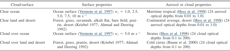
se-lected from a database of plane-parallel, horizontally homogeneous radiative transfer simulations for Earth scenes under a wide range of conditions. For a given surface type and cloud category (clear ocean, cloud over land, etc.), the specific theoretical radiances in Eq. (7) are determined from the model simulation that mini-mizes the root-mean-square difference in radiance be-tween theory and observations in the angular bins for which data are available. In the SW, the radiative trans-fer calculations are based on the discrete-ordinate-meth-od radiative transfer cdiscrete-ordinate-meth-ode (DISORT; Stamnes et al. 1988); in the LW, radiances are based on a code by Gupta et al. (1985). The appendix describes the cases that compose the theoretical radiance database.
To determine Fj, the usual approach is to integrate jexplicitly, using a discrete form of Eq. (4). However,
I
as pointed out by Loeb et al. (2002), radiance contri-butions from the entire Earth disk and overlying at-mosphere must be taken into account, including radi-ances that emerge from the atmosphere along slant at-mospheric paths beyond Earth’s horizon (i.e., above Earth’s tangent point). Ignoring these radiance contri-butions can cause 1–2 W m22underestimation in TOA
flux. To account for these contributions, Loeb et al. (2002) showed that the FOV reference level must be defined at least at 100 km above Earth’s surface. To convert the viewing zenith angle from a surface FOV reference level to a 100-km FOV reference level, the following transformation is used:
re1 hsfc
sinu(h100)5
1
2
sinu(h ),sfc (8)re 1h100
whereu(hsfc) is the viewing zenith angle at the surface
reference level, and reis the mean radius of Earth (which
is set to 6371 km).
At a 100-km FOV reference level, the CERES
cen-troid intersects Earth’s surface for angles u(h100)
be-tween 08 and 79.98 (region I in Fig. 4), where u(h100)
denotes viewing zenith angles defined at the 100-km FOV reference level. For this range of angles,Ijis
de-termined from the measurements, as described above. Foru(h100) of greater than 79.98, the CERES footprint
centroid lies beyond the Earth tangent point, and the number of CERES footprints in the SSF at these angles is limited because of the narrow VIRS swath. For clear scenes, as u(h100) increases beyond 79.98, the radiance
decreases rapidly and eventually approaches zero as CE-RES begins to observe cold space. To estimate radiances foru(h100) . 79.98, moderate-resolution transmittance
model and code (MODTRAN) (Kneizys et al. 1996) simulations for a molecular atmosphere are used. If the scene type is cloudy, however, the MODTRAN molec-ular atmosphere approximation is only used at observer viewing zenith angles for which the FOV centroid lies above the cloud top (region III in Fig. 4). The cloud-top height is given by the average effective cloud-cloud-top height of all footprints in the ADM class. For most clouds, the observer viewing zenith angle corresponding to the cloud top is close to that for the Earth tangent point [i.e., u(h100) 5 79.98]. For example, for a cloud
u(h100)580.78. In the narrow range of angles between
the Earth tangent point and cloud top (region II in Fig. 4), radiances are extrapolated from radiances atu(h100) , 79.98.
The reflected shortwave and emitted longwave ADM fluxes are determined as follows:
SW
where wk and wlare Gaussian quadrature weights for
integration over viewing zenith angles from 08 to 908
and relative azimuth angles from 08 to 1808, respec-tively. The number of Gaussian quadrature points (i.e.,
Nk and Nl) used to evaluate Eqs. (9) and (10) is 200.
Radiances at the Gaussian points are determined by lin-early interpolating the mean radiances defined over the CERES angular bins.
Because the viewing geometry and footprint geolo-cation in the SSF product are provided at the surface reference level, the CERES ADMs are defined so that they also correspond to the surface reference level. The SW and LW ADMs at the surface reference level are given by
Because Ij in Eq. (6) is inferred from daily mean
radiances, an estimate of the variability in the SW ADMs can be inferred from the standard deviation in daily mean radiances as follows:
s (u ,u,u)
p Ij oi k l
«Rj(uoi,uk,ul)5 tp,n
[
]
, (13)F (j uoi) ÏN (Ij uoi,uk,ul)
where tp,nis the 100 (12p)th percentile of the Student’s
t distribution with n degrees of freedom, and sIj, and
N , are the standard deviation and number of daily meanIj
radiances in an angular bin, respectively. For the 95% confidence interval, p 5 0.025 and n 5 (NIj 2 1). A similar expression can also be used to estimate the var-iability in LW ADMs. Note that Eq. (13) is only an estimate of the ADM variability—the actual ADM var-iability would require knowledge of the standard de-viation in daily mean anisotropic factors rather than the mean radiances.
5. Instantaneous TOA flux estimation
a. Interpolation bias correction
To estimate a flux from a radiance measurement, the appropriate ADM scene type must first be determined from the imager retrievals. Next, Eq. (5) is applied using an estimate of the anisotropic factor. However, because the anisotropy of Earth scenes generally varies with view-ing geometry and cloud/clear-sky properties in a contin-uous manner, whereas the CERES ADMs [Eqs. (11) and (12)] are defined for discrete angular bins and scene types, an adjustment to the CERES anisotropic factors is needed to avoid introducing large instantaneous flux er-rors or sharp flux discontinuities between angular bins or scene types. One way of reducing angular bin dis-cretization errors is to obtain anisotropic factors by lin-early interpolating bin-average ADM radiances [e.g., (uoi, uk, fl; hsfc)] and fluxes [e.g., (uoi; hsfc)] to SW
SW
Ij Fj
each observation angle (uo,u,f) and evaluating
aniso-tropic factors from Eq. (6) using the interpolated quan-tities. In addition, interpolation over other parameters that influence anisotropy (e.g., cloud optical depth) can also be used. In some cases it may even be advantageous to combine empirical and theoretical ADMs to estimate the anisotropic factor at a particular angle (e.g., clear ocean SW ADMs in section 6a).
When linear interpolation is used, the instantaneous TOA flux is given by
pI(uo,u,f; h )sfc
ˆ
F(uo,u,f; h )sfc 5 ˜ , (14)
R (j uo,u,f; h )sfc
where R˜j(uo,u,f; hsfc) represents an anisotropic factor
at the surface reference level determined from inter-polated ADM radiances [I˜j(uo, u, f; hsfc)] and fluxes
[F˜j(uo; hsfc)]. Although instantaneous flux errors are
likely reduced with this approach, there is no guarantee that ensemble averages of the instantaneous fluxes will remain unbiased. A bias in the mean flux will occur if linear interpolation is used when the actual radiance varies nonlinearly within an angular bin. It also occurs when theoretical models are used to supplement em-pirical ADMs. The bias for a specific scene type j in angular bin (uoi,uk,fl) is determined from the
differ-ence between the estimated mean flux and the ADM mean flux (determined by direct integration of radianc-es) as follows:
DF (juoi,uk,fl; h )sfc pI(uo,u,f; h )sfc
5
7
˜8
2 F (juoi; h ),sfc (15)R (juo,u,f; h )sfc ikl
where the first term on the right-hand side is the average of all instantaneous flux estimates from Eq. (14) falling in angular bin [uoi6(Duo)/2,uk6(Duk)/2,fl6(Dul)/
2] for scene type j, and Fj(uoi; hsfc) is the corresponding
FIG. 5. Clear-sky ADM anisotropic factors foruo5308–408for individual IGBP types with moderate-to-high tree/shrub coverage. Positiveucorresponds to forward scattering directions, whereas negativeucorresponds to backscattering.
pI(uo,u,f; h )sfc
ˆ
F9(uo,u,f; h )sfc 5 ˜
R (j uo,u,f; h )sfc
1 dF (juo,u,f; h ),sfc (16) where
dF (j uo,u,f; h )sfc
DF (u ,u,f; h )
I(uo,u,f; h )sfc j oi k l sfc
5 2 . (17)
˜I (j uo,u,f; h )sfc I(u ,u,f; h )
o sfc
˜
7
I (juo,u,f; h )sfc8
iklWhen the ensemble average of instantaneous TOA fluxes from Eq. (16) is determined, the mean flux is unbiased becausedFj(uoi,uk,fl; hsfc)5 DFj(uoi,uk,fl; hsfc). This
procedure is used in all SW TOA flux estimates (except over snow). In the LW and WN channels,dFj(u) is close
to zero and is therefore not explicitly accounted for.
b. TOA flux reference level
Based on theoretical radiative transfer calculations using a model that accounts for spherical Earth geom-etry, Loeb et al. (2002) recently showed that the optimal reference level for defining TOA fluxes in Earth radi-ation budget studies is approximately 20 km. This ref-erence level corresponds to the effective radiative ‘‘top-of-atmosphere’’ because the radiation budget equation is equivalent to that for a solid body of a fixed diameter
that only reflects and absorbs radiation. The TOA flux at the 20-km reference level h20is determined from the
flux at the surface reference level as follows:
2
re
ˆ ˆ
F9(uo,u,f; h )20 5 F9(uo,u,f; h )sfc
1
2
. (18)re 1h20
On the CERES SSF product, instantaneous TOA fluxes are provided only for CERES radiances withu(hsfc)#
708anduo#86.58.
c. Footprints with insufficient imager information
FIG. 6. Same as in Fig. 5 but for low-to-moderate tree/shrub-coverage ADM class.
FIG. 8. Reflectance relative frequency distribution for open shrub and barren desert IGBP types for angular binuo5408–508,u 508– 108, andf 5708–908.
range of the retrieval model (resulting in no-retrievals as-signments), instantaneous TOA fluxes are estimated re-gardless of what the total fraction of unknown cloud prop-erties is over the footprint. TOA flux estimates for these footprints likely have greater instantaneous errors than those derived with complete imager information, but bi-ases in the overall means will be avoided if the errors are random.
To determine a TOA flux for a footprint that lacks suf-ficient imager information to define an ADM scene type, ADM radiances [e.g., (uoi,uk,fl; hsfc)] are interpolated
SW
Ij
to the EOV viewing geometry and are compared with the measured radiance. The anisotropic factor used to convert the measured radiance to flux is evaluated from the ADM whose interpolated radiance most closely matches the mea-sured radiance. To constrain the result, only ADMs having the same underlying surface type as the measurement are considered as possible candidates. From the 9-month CE-RES–TRMM dataset, footprints with insufficient imager coverage to determine an ADM scene type occur approx-imately 7% of the time.
d. Mixed scenes
When a CERES footprint contains a mixture of sur-face types (e.g., ocean and land, land and desert), in-stantaneous TOA fluxes are determined using the ADM that corresponds to the surface type with the highest percent coverage over the footprint. For example, near coastlines, if most of the footprint PSF-weighted area is over ocean, an ocean ADM is used to convert the radiance to flux. In converse, if most of the footprint area is over land, one of the land ADMs is used. An exception occurs when SW TOA fluxes are estimated from mixed land–ocean footprints in the sunlight region. In that case, if the glint angle [Eq. (3)] is#408and the footprint is covered by more than 5% ocean, the foot-print bidirectional reflectance is assumed to be closer to that for ocean, and one of the ocean ADMs is used.
6. SW ADM scene types
a. Clear ocean
Clear footprints are defined as footprints with$99.9% of VIRS imager pixels identified as cloud free. Separate clear ocean ADMs are defined for four intervals of wind speed corresponding to the 0–25th, 25th–50th, 50th–75th, and 75th–100th percentiles of the wind speed probability density distribution. These correspond to wind speed in-tervals of approximately,3.5, 3.5–5.5, 5.5–7.5, and.7.5 m s21. The wind speeds, which correspond to the 10-m
level, are based on Special Sensor Microwave Imager (SSM/I) retrievals (Goodberlet et al. 1990) that have been ingested into the ECMWF data assimilation analysis. For a given wind speed interval wj, the ADM is defined
fol-lowing the procedure outlined in section 4.
Because the anisotropy of clear ocean scenes also
de-pends on aerosol optical depth, this dependence should also be accounted for when estimating SW fluxes over clear ocean. The SSF product provides aerosol optical depth retrievals (Ignatov and Stowe 2002), but only in viewing conditions for which the glint angle exceeds 408. It is consequently not possible to construct empirical ADMs stratified by the Ignatov and Stowe (2002) aerosol optical depth retrievals because no information on how CERES radiances vary with aerosol optical depth in the glint region is available. As an alternative, instantaneous TOA fluxes are first inferred in any viewing geometry from wind speed–dependent empirical ADMs. Next, these TOA flux estimates are adjusted as follows:
pI(uo,u,f; h )sfc
speed–dependent ADMs, and Rth(w
j, I) and Rth(wj, I˜) are
anisotropic factors inferred from the measured CERES radiance I(uo,u,f; hsfc) and the interpolated ADM radiance f; hsfc) are compared with lookup tables of theoretical SW
radiances stratified by aerosol optical depth. Here, Rth(w j,
I) and Rth(w
j, I˜) correspond to the aerosol optical depth
FIG. 9. The SW flux difference over (a) dark and (b) bright desert, and rms SW flux difference over (c) dark and (d) bright desert attributable to differences between CERES, ScaRaB, and ERBE desert ADMs against solar zenith-angle bin midpoint. Solar zenith angle bins are based on the ERBE definition given by: 08–25.88, 25.88–36.98, 36.98–45.68, 45.68–53.18, 53.18–60.08, 60.08–66.48, 66.48–72.58, 72.58–78.58, and 78.58–84.38.
subroutine from the 6S radiative transfer code (Vermote et al. 1997). This routine accounts for specular reflection (Cox and Munk 1954), wind speed–dependent whitecaps (Koepke 1984), and below–water surface reflectance (Mo-rel 1988).
Equation (19) can be used to estimate TOA flux in any viewing geometry. However, as the satellite viewing geometry moves towards the ocean specular reflection direction, the radiance increase for a change in angle as small as 18 can be very large. Because such changes are unresolved by the relatively coarse angular bins used to define CERES ADMs, instantaneous TOA flux es-timates are generally unreliable for footprints near the specular reflection direction. As a consequence, the ra-diance-to-flux conversion is not performed in these re-gions. However, ignoring these samples (e.g., by not providing a TOA flux estimate) can introduce biases in regional mean fluxes because fluxes over cloudy por-tions of a region will contribute disproportionately to
the overall regional mean. To avoid this bias, fluxes in cloud-free sunlight are given by the clear ocean wind speed–dependent ADM flux (FSW) interpolated at the
j
solar zenith angle of the observation.
To determine whether a footprint is too close to the specular reflection direction to provide a reliable flux retrieval, the derivatives of clear ocean ADM aniso-tropic factors with respect to illumination and viewing geometries (]Rj/]uo,]Rj/]u, and ]Rj/]f) are evaluated
in each CERES angular bin. If an observation falls in an angular bin for which one of the derivatives exceeds a threshold value, a radiance-to-flux conversion is not performed. In this study, a threshold of 0.075 per degree is used as the cutoff, which corresponds approximately to a 408 glint angle threshold.
b. Clear land and desert
FIG. 10. Anisotropic factors foru 508–158ERBE angular bin against solar zenith angle for CERES, ScaRaB, and ERBE SW ADMs for relative azimuth angle bins (a) 08–98, (b) 98–308, (c) 308–608, (d) 608–908, (e) 908–1208, (f ) 1208–1508, (g) 1508–1718, and (h) 1718–1808.
vegetation coverage, surface type, and surface hetero-geneity (Roujean et al. 1992). The intervening atmo-sphere modifies the surface anisotropy, particularly at shorter wavelengths (Zhou et al. 2001) and for large aerosol optical depth (Li et al. 2000). The observed anisotropy of TOA-leaving radiances also depends on instrument resolution, because clear land scenes become more inhomogeneous when observed at larger spatial scales.
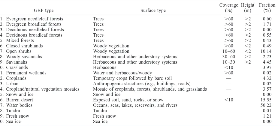
The inclined orbit of the TRMM satellite provides a unique opportunity for determining ADMs under all so-lar zenith angle conditions. To account for climatolog-ical differences between surface types, ADMs are first constructed for each of the International Geosphere Bio-sphere Programme (IGBP) Global Land Cover types (Loveland and Belward 1997) for which there are suf-ficient data in the Tropics. CERES uses a 109 latitude by 109 longitude map of IGBP types that covers the globe (D. A. Rutan and T. P. Charlock 2001, personal communication). The IGBP classification scheme is pro-vided in Table 1, along with the fraction of cloud-free CERES footprints for each IGBP surface-type category over the entire 9 months of daytime CERES–TRMM observations (last column). Over land and desert, barren desert (16) and open shrubs (7) account for 53% of the clear footprints, IGBP types with low-to-moderate tree/ shrub coverage (i.e., IGBP types 9–14) account for 34%, and IGBP types with moderate-to-high tree/shrub
cov-erage (i.e., IGBP types 1–6 and 8) account for 13%. It is unfortunate that there are not enough data over the Tropics to construct ADMs for deciduous needleleaf forests (3), permanent wetlands (11), and urban (13) IGBP types.
Figures 5 and 6 show clear-sky ADM anisotropic factors for uo 5 308–408 for individual IGBP types
TABLE1. IGBP-type classification scheme. Coverage refers to the fractional coverage of a surface type over 131 km2area. Height refers
to the height of the vegetation. Fraction refers to the cloud-free CERES footprints in each IGBP type over the entire 9 months of daytime CERES–TRMM observations.
IGBP type Surface type
Coverage 1. Evergreen needleleaf forests
2. Evergreen broadleaf forests 3. Deciduous needleleaf forests 4. Deciduous broadleaf forests 5. Mixed forests
Herbaceous and other understory systems Herbaceous and other understory systems Herbaceous
14. Cropland/natural vegetation mosaics 15. Snow and ice
Water and herbaceous/woody Temporary crops followed by bare soil Anthropogenic structures (e.g., buildings, roads) Mosaic of croplands, forests, shrublands, and grasslands Snow and ice
Exposed soil, sand, rocks, or snow Oceans, seas, lakes, reservoirs, and rivers Tundra
SSF only retains footprints within the VIRS swath, oblique viewing zenith angles are only sampled when CERES is in RAP or along-track mode, which only occurs every third day of data acquisition).
To reduce errors in flux attributable to poorly sampled ADM angular bins, the CERES ADMs are constructed using the low-to-moderate and moderate-to-high tree/ shrub coverage classes to determine fluxes over land. For these cases, the variability in the anisotropic factors is estimated to be less than 0.04 at the 95% confidence level for most solar zenith and viewing zenith angle bins. The variability in anisotropic factors is estimated from the variability in daily mean radiances for each angular bin [Eq. (13)].
ADM anisotropic factors for uo5 308–408 for two
IGBP types characteristic of desert regions are presented in Fig. 7. Open shrubs (7) are prevalent over west and central Australia, the southwest parts of North America, South America, and Africa, and in central Asia. Barren deserts (16) are associated primarily with the Saharan, Arabian, Thar, and Gobi deserts. As shown in Fig. 7, ADMs are different for these two IGBP types. The ADMs over barren desert regions are more isotropic, presumably because of the lower vegetation coverage there. Capderou (1998) showed similar differences based on ScaRaB measurements from the Meteor-3-07 satellite.
To examine how well the IGBP classification sepa-rates the two classes of desert, relative frequency dis-tributions of SW reflectance were determined in each angular bin. Shortwave reflectance is inferred from a measured SW radiance as follows:
r(uo,u,f; h )sfc
tance at the time of observation, and do is the mean
Earth–Sun distance.
Figure 8 shows results for angular binuo5408–508, u 5 08–108, and f 5 708–908. The two desert types have a well-defined primary peak at reflectances near 15% (open shrubs) and 30% (barren desert), there is a secondary peak in the barren desert distribution near 15%, and there is a hint of a secondary peak in the open shrubs distribution at reflectances near 25%. The reason for the multiple peaks in the two reflectance distribu-tions may be because the fixed IGBP map cannot ac-count for annual or seasonal changes in vegetation type and cover. To provide a better separation between the two desert types, all CERES footprints in 109 desert regions are reclassified as either ‘‘dark’’ or ‘‘bright’’ desert. Regions with CERES SW reflectances closer to the primary peak of the open shrubs reflectance distri-bution are classified as dark desert, whereas regions with CERES SW reflectances closer to the primary peak of the barren desert reflectance distribution are classified as bright desert.
FIG. 11. Frequency of occurrence of (a) liquid water and (b) ice cloud ADM classes by cloud fraction and cloud optical depth.
the barren desert ADMs, particularly in the forward scattering direction, for which differences in anisotropic factors can reach 6%. In addition, for both desert types, the ADM variability estimate [Eq. (13)] is much smaller for the new dark and bright desert classes. For these cases, the variability in the anisotropic factors is esti-mated to be less than 0.03 at the 95% confidence level for most solar zenith and viewing zenith angle bins.
Capderou (1998) recently constructed clear desert ADMs using measurements from the ScaRaB instru-ment on board the Meteor-3-07 satellite. Using scene identification based on the ERBE maximum likelihood estimation (MLE) technique (Wielicki and Green 1989) to identify clear scenes over the Saharan, Arabian, Na-mib–Kalahari, and Australian deserts, Capderou (1998) derived ADMs for dark and bright desert conditions. To compare the ScaRaB and CERES ADMs, the CERES ADMs are adjusted to the midpoint of the ScaRaB ADM angular bins (ScaRaB uses the same angular bin defi-nition as ERBE) by interpolating CERES ADM mean radiances (ISW)and fluxes (FSW) to the angular bin
mid-j j
points and inferring the anisotropic factors from the ra-tio. The ScaRaB–CERES ADM differences are con-verted to equivalent SW flux differences by inferring fluxes from the CERES ADM mean radiances (ISW)
us-j
ing both sets of ADMs in each ScaRaB ADM angular
bin (u . 758 excluded) as though the radiances were instantaneous values. Figure 9 shows the resulting SW flux differences and root-mean-square (rms) differences as a function of solar zenith angle inferred from all angular bins. Also provided are results comparing fluxes based on ERBE (Suttles et al. 1988) and CERES desert ADMs. For solar zenith angle bins ,608, the ScaRaB and ERBE fluxes are generally within 3 W m22of the
CERES fluxes for both the dark and bright desert mod-els. At larger solar zenith angles, both the ScaRaB and ERBE fluxes are lower than the CERES fluxes by up to 7 W m22.
FIG. 12. Overcast ice cloud ADMs with cloud optical depths between (a) 1.0 and 2.5 and (b) 20 and 25 foruo5508–608. (c), (d) Differences in anisotropic factors between liquid water and ice clouds (liquid2ice) for the same cloud optical depth intervals as (a) and (b).
zenith angle–dependent bias in the MLE scene identi-fication.
c. Clouds over ocean
The ADM scene-type stratification for clouds over ocean is provided in Table 2. There are two phase cat-egories, 12 cloud-fraction catcat-egories, and 14 cloud-op-tical-depth categories. Phase over a CERES footprint is inferred from VIRS-imager pixel-level phase retrievals (Minnis et al. 1998). Each VIRS-imager pixel within a CERES cloud layer is assigned a phase index of 1 for liquid water and 2 for ice. The pixel-level phase indices are weighted by the CERES PSF to yield the effective phase over each layer. The effective phase over the en-tire footprint is determined by area-averaging the phase indices of each layer using Eq. (1). ADMs for ‘‘liquid clouds’’ are determined from footprints with an effective phase index,1.5, and ADMs for ‘‘ice clouds’’ are de-termined from footprints with an effective phase index
$1.5. A separate class for ‘‘mixed-phase’’ footprints would be desirable, but the sampling is limited, with only 9 months of CERES–TRMM observations.
Although the number of ocean cloud ADM scene types can potentially reach 336 (i.e., 2312314), the actual number of scene types with sufficient data is much lower. In most solar zenith angle bins, 72 (or 43%) of the possible liquid water cloud classes have sufficient data to build an ADM, whereas 57 (or 34%) of the possible ice cloud classes have sufficient sampling. Fig-ures 11a and 11b show the frequency of occurrence of liquid water and ice cloud ADM classes, respectively, by cloud fraction and cloud optical depth. When cloud fraction is low, only the thin ADM cloud classes are sampled. As the cloud fraction increases, the range in cloud optical depth increases, and more cloud-optical-depth ADM classes appear. A similar broadening in cloud-optical-depth distributions with cloud cover was also observed by Barker et al. (1996).
TABLE2. Shortwave ADM scene-type parameter intervals for clouds over ocean, land, and desert.
Surface type
PSF-weighted
phase index Cloud fraction Cloud optical depth
Ocean ,1.5 (liquid water)
.1.5 (ice)
0.1–10, 10–20, 20–30, 30–40, 40–50, 50–60, 60–70, 70– 80, 80–90, 90–95, 95–99.9, 99.9–100
0.01–1.0, 1.0–2.5, 2.5–5.0, 5.0–7.5, 7.5–10, 10–12.5, 12.5–15, 15–17.5, 17.5–20, 20–25, 25–30, 30–40, 40– 50,.50
Moderate–high tree/shrub coverage; low–moderate tree/shrub coverage, dark desert; bright desert
,1.5 (liquid water)
.1.5 (ice)
0.1–25, 25–50, 50–75, 75– 99.9, 99.9–100
0.01–2.5, 2.5–6, 6–10, 10–18, 18–40,
.40
FIG. 13. The SW ADM anisotropic factors interpolated to ERBE angular bins for overcast ice clouds as a function of cloud optical depth, viewing zenith angle, and relative azimuth angle foruo553.1–60. Circles denote the ERBE overcast ADM.
in the overcast (99.9%–100%) cloud-fraction class. If only footprints dominated by liquid water clouds (i.e., footprint effective phase index ,1.5) are considered, the fraction of overcast footprints drops to 25%, as com-pared with 72% for footprints dominated by ice clouds (i.e., footprint effective phase index$1.5). Overall, the frequency of occurrence for the liquid water cloud class is 75%, as compared with 25% for the ice cloud class. Examples of ADMs for thin (cloud optical depths of 1.0–2.5) and thick (cloud optical depths of 20–25) ice clouds for uo 5 508–608 are provided in Figs. 12a,b.
For the thin-cloud case (Fig. 12a), the anisotropic factor ranges from 0.6 to 3.3 as compared with 0.9 to 1.6 for the thick-cloud case. The largest sensitivity to cloud optical depth occurs at near-nadir views, for which the anisotropic factor changes by 50%. Figures 12c,d show differences in anisotropic factors between liquid water
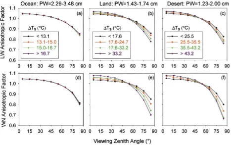
FIG. 14. Daytime clear-sky LW and WN ADMs for the 33d–66th-percentile interval of precipitable water. ADMs are shown for the LW channel over (a) ocean, (b) land, and (c) desert and for the WN channel over (d) ocean, (e) land, and (f ) desert. Here DTsis the vertical temperature difference, which corresponds to the lapse rate in the first 300 hPa of the atmosphere above the surface.
Figure 13 compares CERES ADMs for overcast ice clouds for each of the 14 cloud-optical-depth intervals together with the one ERBE overcast ADM. For this comparison, the CERES ADMs are interpolated to the midpoints of the ERBE angular bins (Suttles et al. 1988). The ERBE overcast model most closely follows the CE-RES ADM for cloud-optical-depth interval 12.5–15. The ERBE anisotropic factors exceed CERES values by up to 60% for thin clouds near nadir; for viewing zenith angles between 408and 608, anisotropic factors are in-sensitive to cloud optical depth, consistent with theo-retical simulations by Davies (1984).
Because of the strong sensitivity in the anisotropic factors to cloud properties (i.e., cloud optical depth and cloud fraction), the ADM lookup tables under cloudy conditions are interpolated not only to the measurement viewing geometry, but also to the effective cloud frac-tion and cloud optical depth over the footprint. The interpolation procedure is the same as that outlined in section 5a but involves interpolation over two extra var-iables.
d. Clouds over land
The ADM classes for cloudy conditions over land are stratified by the four land types considered for clear
conditions (section 6b), two cloud-phase classes (de-fined in the same manner as for clouds over ocean), five cloud-fraction classes and six cloud-optical-depth clas-ses (Table 2). Because only 9 months of CERES– TRMM measurements are available, the number of clas-ses over each of the land types is reduced relative to that over ocean to ensure a sufficient number of samples to construct an ADM.
e. Snow
Because the TRMM orbit is restricted to 358S–358N, sampling under snow conditions is insufficient for de-veloping empirical ADMs. As an alternative, fluxes un-der snow conditions for CERES–TRMM are determined from theoretical ADMs based on 12-stream DISORT (Stamnes et al. 1988) model calculations. In the cal-culations, the surface bidirectional reflectance of snow is accounted for explicitly by inserting a packed snow layer at the bottom of the atmosphere (0–1-km altitude). Within the snow layer, ice particles are assumed to be spheres, having a lognormal size distribution with a mode radius of 50mm and a standard deviation of 2.0
mm. The concentration of ice particles is 1.0 3 1012
m23, which corresponds to a density ofø0.5 Mg m23.
TABLE3. Longwave and WN ADM scene-type parameter intervals for clear, broken, and overcast scenes.
Overcast All ,33
33–66
compute the optical properties of ice particles from Mie theory. The atmosphere is divided into six layers. Ab-sorption by water vapor, ozone, carbon dioxide, and oxygen are based on k-distribution tables (Kato et al., 1999) based on a midlatitude summer atmosphere (McClatchey et al. 1972).
Under cloudy conditions, a liquid water cloud layer between 1 and 2 km is inserted above the snow layer in the DISORT model calculations. The cloud particles are also taken to be spheres, having a lognormal dis-tribution with a mode radius of 10 mm and standard deviation of 1.42mm. The cloud optical depth is fixed at 10. Radiances are computed at 18 solar zenith angles, 51 viewing zenith angles, and 61 relative azimuth an-gles. TOA fluxes from the theoretical ADMs are deter-mined using Eq. (14).
7. LW and WN ADM scene types
For CERES, LW and WN ADMs are defined inde-pendent of the SW ADMs. This approach differs from that of ERBE, which uses the same scene types for both the SW and LW ADMs. CERES LW and WN ADMs are determined for scene types defined by meteorolog-ical parameters and imager-based cloud parameters that influence LW and WN radiance anisotropy of Earth scenes. As a result, the ERBE method of defining LW ADMs by colatitude is not used in CERES since lati-tudinal and seasonal variations in anisotropy are ac-counted for on a footprint-by-footprint basis from col-located meteorological and imager-based parameters. Also, because the cloud retrieval algorithm uses a dif-ferent method at night than it does during the daytime, CERES ADMs are determined separately for daytime and nighttime conditions.
The LW and WN ADMs are divided into broad
cat-egories based on cloud cover (clear, broken, and over-cast) and surface type (ocean, land, and desert). Each of these categories is further stratified by intervals of precipitable water, cloud fraction, vertical temperature change, and cloud infrared emissivity (Table 3). To en-sure that there is sufficient sampling for every scene type, the parameters are stratified according to their fre-quency distributions using fixed percentile intervals rather than fixed discrete intervals. The percentile ap-proach allows the data to define the width and range used to stratify a given parameter, thereby ensuring that each ADM scene type is adequately sampled.
a. LW and WN ADM scene-type parameters
Cloud categories are based on the imager-derived cloud fraction over the CERES footprint. A footprint is assumed to be clear when the cloud fraction is#0.1%. ‘‘broken’’ when the cloud fraction is between 0.1% and 99.9%, and ‘‘overcast’’ when the cloud fraction is
$99.9%. In Table 3, ocean is defined by IGBP type 17 (Table 1), desert is defined by IGBP types 7 and 16, and land is all IGBP types except 7, 15, 16, 17, 19, and 20. Over snow, empirically derived LW and WN ADMs are unavailable because of inadequate sampling. There-fore, fluxes for footprints over snow are estimated in the same manner as footprints with insufficient imager information (section 5c).
Precipitable water in Table 3 is the water vapor burden from the surface to the TOA. For scenes over water, the data source for precipitable water is the SSM/I dataset, if available. If SSM/I data are unavailable or the foot-print is over land, ECMWF precipitable water is used. Under clear conditions, the vertical temperature change (DTs) corresponds to the lapse rate in the first 300 hPa
FIG. 15. The LW and WN anisotropic factors for the 08–108viewing zenith angle bin over desert as a function ofDTsin each precipitable water interval. Anisotropic factors are provided for (a) daytime LW, (b) nighttime LW, (c) daytime WN, and (d) nighttime WN. Physical values ofDTscorresponding to each percentile interval are provided in Table 4.
subtracting the air temperature at the pressure level that is 300 hPa below the surface pressure (i.e., surface pres-sure minus 300 hPa) from the imager-based surface skin temperature. A separate ADM class is produced when there is an inversion in the boundary layer (DTs,08C).
When clouds are present in a CERES footprint, vertical temperature change (DTc) refers to the difference in
temperature between the surface and cloud;DTcis
com-puted by subtracting the imager-based effective (equiv-alent blackbody) cloud-layer temperature from the un-derlying skin temperature. If the imager-based surface skin temperature is unavailable (e.g., overcast condi-tions), a skin temperature from the ECMWF data as-similation model is used.
The mean infrared emissivity for a cloud layer is defined as the ratio of the difference between the ob-served and clear-sky VIRS 11-mm radiances to the dif-ference between the cloud emission and clear-sky ra-diances. The clear-sky radiance is determined either from surrounding cloud-free observations when avail-able, or from ECMWF surface skin temperature, surface
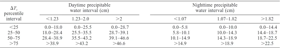
TABLE4. TheDTs(8C) intervals corresponding to each percentile interval in Fig. 14 for clear daytime and nighttime desert.
DTs percentile
interval
Daytime precipitable water interval (cm)
,1.23 1.23–2.0 .2
Nighttime precipitable water interval (cm)
,1.07 1.07–1.82 .1.82
,25 25–50 50–75
.75
0.0–18.0 18.0–28.4 28.4–38.9
.38.9
0.0–25.5 25.5–35.5 35.5–43.2
.43.2
0.0–28.7 28.7–39.1 39.1–46.6
.46.6
0.0–5.8 5.8–10.1 10.1–14.9
.14.9
0.0–10.0 10.0–14.3 14.3–18.9
.18.9
0.0–14.4 14.4–18.7 18.7–22.5
.22.5
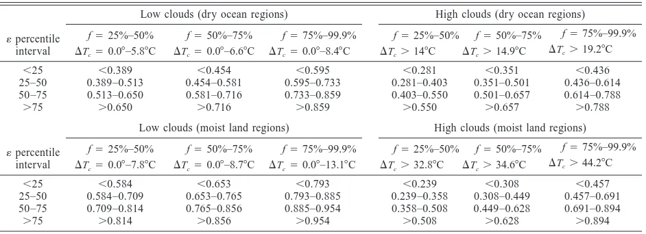
FIG. 16. The LW anisotropic factors for the 08–108viewing zenith angle bin for broken clouds as a function of cloud emissivity in each cloud fraction interval: (a) low clouds over dry ocean regions (0–20thDTcpercentile interval and 0–33d precipitable water interval), (b) high clouds over dry ocean regions (80th–100thDTcpercentile interval and 0–33d precipitable water interval), (c) low clouds over moist land regions (0–20thDTcpercentile interval and 66th–100th precipitable water interval), and (d) high clouds over moist land regions (80th– 100th DTcpercentile interval and 66th–100th precipitable water interval). Physical values corresponding to each percentile interval are provided in Table 5.
b. ADM sensitivity to scene type
Figure 14 provides examples of LW and WN ADMs for clear scenes over ocean, land, and desert as a func-tion ofDTsfor the 33d–66th-percentile interval of
pre-cipitable water. TheDTsintervals correspond to the 0–
25th-, 25th–50th-, 50th–75th-, and.75th-percentile
in-tervals (there was not sufficient sampling to construct ADMs for inversion conditions). The range of DTsis
much smaller over ocean than it is over land and desert because DTs has a much narrower distribution over
ocean. As DTs increases, LW and WN anisotropy
TABLE5. The«intervals corresponding to each percentile interval considered in Fig. 15 for broken cloud conditions over ocean and land.
«percentile interval
Low clouds (dry ocean regions) f525%–50%
High clouds (dry ocean regions) f525%–50%
Low clouds (moist land regions) f525%–50%
High clouds (moist land regions) f525%–50%
FIG. 17. The LW anisotropic factors for the 08–108viewing zenith angle bin for overcast clouds as a function of cloud emissivity in each precipitable water interval: (a) low clouds (0–20thDTcpercentile interval) and (b) high clouds (80th–100thDTcpercentile interval). Physical values corresponding to each percentile interval are provided in Table 6.
anisotropic factors to DTsoccurs close to nadir, where
it varies byø2%, which corresponds to a LW flux var-iation of ø6 W m22. Sensitivity to DT
s is more
pro-nounced for the WN channel because of its larger de-pendence on surface temperature.
LW and WN anisotropies change between daytime and nighttime conditions over clear desert regions (Figs. 15a– d). Because daytime surface temperatures are so much larger than those at night, the magnitude ofDTsin each
percentile interval is greater during the daytime (Table 4). The daytime LW and WN anisotropy is consequently stronger than at night. Based on these results, ignoring daytime/nighttime differences in anisotropy would lead to a 5 W m22bias in the day–night LW flux difference.
In broken cloud conditions, LW anisotropy shows a slight dependence on cloud infrared emissivity (Fig. 16,
Table 5). Sensitivity to«increases with cloud cover and cloud height, particularly over moist land. In general, LW anisotropy increases with decreasing«. This trend is most pronounced for overcast conditions, as illustrated in Fig. 17 (see also Table 6), which shows nadir anisotropic fac-tors for low and high overcast clouds. Clouds that occur in the wettest (largest precipitable water) regions with the largestDTcshow the strongest sensitivity to«. Anisotropic
factors range from 1.02 for thick high clouds to 1.158 for thin high clouds in the moist regions. Thisø13% differ-ence in anisotropic factor corresponds to a differdiffer-ence in LW flux of 25 W m22for these clouds.
8. Summary