Sept.-Oct
TIME SERIES MODELING AND FORECASTING OF THE CONSUMER PRICE
INDEX BANDAR LAMPUNG
1*Faiga Kharimah, 1Mustofa Usman, 1Widiarti and 2Faiz AM. Elfaki 1
Departement of Mathematics, Lampung University 2
Department of Science, Faculty of Engineering, IIUM, Malaysia *E-mail: [email protected]
ABSTRACT:The aims of this study are to find the best Time Series model for forecasting the Consumer Price Index (CPI). To
find the best model, first we evaluate the stationary of the data by using time series plot, Autocorrelation Function (ACF), and Unit root Test. Then the Time Series model was found by using ACF and Partial Autocorrelations Function (PACF). The best model was found by using the criteria: Mean Squares Error (MSE), Akaike Information Criteria (AIC) and Bayesian Information Criterion (BIC. Based on this criteria the best modelfound in this paper is ARIMA (1,1,0) compare to ARIMA (0,1,1), and ARIMA(1,1,1).
Key words : Time Series Modeling; CPI; Forecast; ARIMA; ACF; PACF.
1. INTRODUCTION
Consumer Price Index (CPI) may be regarded as a summary statistic for frequency distribution of price relative. It is the weighted arithmatic mean of the distribution of successive months or years. CPI number measures changes in the general level of prices of a group of commodities. It thus measures changes in the purchasing power of money [1, 2]. Mendenhall [3] states that CPI is a weighted aggregate index that is computed and published monthly. In American experiences Boskin,et.al [4] explains that the CPI program focuses on consumer expenditures on goods and services out of disposable income. Hence, it excludes non-market activity, broader quality of life issues, and the costs and benefits of
One of the methods that commonly used for forecasting time series data is Autoregressive Integrated Moving Average
(ARIMA) [5, 6, 7, 9, 10]. The ARIMA model was developed by George Box dan Gwilym Jenkins [11] and it is called time series method of Box-Jenkins. In their book, Box and Jenkins [11] strongly recommend that forecasts of ARIMA processes be made using the Difference Equation form because it is the simplest approach. Many studies have been done to analyze data CPI. Subhani and Panjwani [2] study about monthly government bonds response to announcements of CPI. Adam, et.al [12] studied CPI in Nigeria by using ARIMA model. Hamid and Tej [3] studied about analyses the seasonality in the monthly consumer price index (CPI) over the period January 1913 to December 2003. Fengwang, et.al [13] study to analyze time series data of CPI in China from January 1995 to May 2008 by ARMA model. In this study the ARIMA model will be used to analyze time series data and forecasting for the CPI in Bandar Lampung City from 2009-2013.
2. TIME SERIES MODELING 2.1. MODEL SPECIFICATION
The model used in this study is the ARIMA. To test for the stationary of data we used time series plot, autocorrelation function(ACF), and unit root test. After the stationarity of the time series was attained, ACF and PACF (partial
autocorrelation function) of the stationary series are employed to select the order of the Autoregressive (AR) process and the order of the Moving Average (MA) process of the ARIMA model. Integrated (I) process, which account for stabilizing or making the data stationary. In practice, one or two level of differencing are often enough to reduce a nonstationary time series to apparent stationarity[14, 15, 16, 17]. The data used in this study are from the Central Bureau of Statistics Indonesia, Lampung Province from 2009 to 2013. It is the monthly data of Consumer Price Index (CPI) of Bandar Lampung City from 2009 to 2013.
2.2. ARIMA MODEL
Step 1:The plot of the stationary data , the data will move fluctuation which are fixed or constant and with no trend. But if the data move fluctuated and not constant, we call the data nonstationary in variance. To make the data stationary in variance we can use Box-Cox transformation [9, 14, 16]. If the stationary in variance of the data have been attain, but there is still a trend in the data, then we can apply differencing to attain the stationary in the mean [4].
Step 2:If the stationary of the data have been attained then we can continue to estimate the order of AR and MA which can be found from the graph of Autocorrelation Function
Step 3: Estimation of model: This deal with estimation of the ARIMA model identified in step 2. The estimation of model parameters can be done by the conditional least square method.
Step 4: Diagnostic checking: The model is checked by analyzing the residual. If the residual are white noise, then we accept the model.
3. EMPIRICAL ANALYSIS AND RESULT 3.1. IDENTIFICATION
Sept.-Oct
Time series plot
Figure 1: Time series plot of CPI series
Figure 1 shows that the plot of data has stationary in variance, but the data not stationary in mean ( there is a trend in the series).
ACF plot
Figure 2: ACF of CPI series
Figure 2 shows that at lag 0, 1, 2, 3, 4, and 5 the bar beyond the significant line, so there are significant autocorrelation at lag 0, 1, 2, 3, 4, and 5. Beside that at lag 5 and 6, the bar still far from zero, so we can conclude that the CPI is not stationary.
Unit root test
Figure 3: Unit root test of CPI series
Hypotheses:
H0 = CPI nonstationary H1 = CPI stationary
Figure 3 shows that the bar at lag 0,1, 2, 3, 4, and 5 in the graph of the unit root test are below the significant line at α = 0,05. The p-value at lag 0, 1, 2, 3, 4, and 5 are greater than 0,1 even very close to 1. Therefore we do not reject the null hypotheses and we conclude that the data are non stationary. After we identified the data, it is known that from the time series plot the data are stationary in varianc, but not stationary in mean. To make sure that the data satisfied the stationary in variance, we check by Box-Cox transfor-mation.
The Box-Cox transformation conducted by first we find the value of the best 𝜆 which will be used in the transformation. The following table is the output from software SAS 9.0 to find the best value of 𝜆.
Table 1: The value of 𝜆
Transformation Information for BoxCox(y)
Lambda R-Square Log Like transformation
-1.000 0.99 -32.4740
1
/
z
-0.500 0.99 -4.2136
1
/
z
0.000 1.00 35.2074
ln
z
0.500 1.00 102.1001
z
1.000 + 1.00 Infty <
z
< - Best Lambda* - Confidence Interval + - Convenient Lambda
The best vaue of 𝜆 from Table 1 above is 𝜆 = 1, therefore
by
z
transformation or since 𝜆 = 1 we can say that we do not need to conduct a transformation. So by using 95% level of significant we can say that the data are stationary in variances.The next to make the stationary in the mean, we do the differencing on the data which has been transformed by Box-Cox transformation with 𝜆 = 1, after the first differencing on the data than we check the stationary through the time series plot, the ACF plot and the unit root test.
Time series plot
Figure 4: Time series plot of first differencing Box-Cox(1) CPI
Figure 4 shows that the time series plot of CPI which has been transformed by using Box-Cox transformation with 𝜆 = 1 and first differencing show that the data are stationary. The ACF graph
Sept.-Oct
Figure 5 shows that the bar at lag 0 and 1 beyond the significant line, so we can say that there is autocorrelation at lag 0 and 1. At lag 5 and 6 the bar around 0, so the data are stationary.
Unit Root Test
Figure 6: Unit root test of first differencing Box-Cox(1) CPI
Hypotheses :
H0 = first differencing Box-Cox (1) CPI nonstationary. H1 = first differencing Box-Cox (1) CPI stationary.
Figure 6, shows that the bar on lag 0,1, 2, 3, 4 and 5 are above the significant line of the unit root test. We see the p-value at lag 1,2,and 3 are close to 0.001, while at lag 4 and 6 the p-value are between 0.01 and 0,001. So we conclude that we reject the null hypotheses and the data are stationary. 3.2. IDENTIFICATION OF ARIMA MODEL
Since the data are stationary, then the asumption of the ARIMA model are satisfied, to find the best ARIMA model for the data, we see the ACF and PACF graphs.
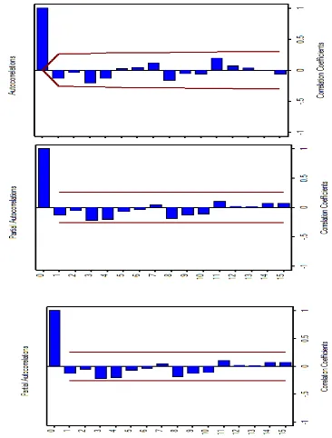
Figure 7: ACF and PACF of first differencing Box-Cox(1) of CPI
Figure 7, shows that the CPI data which has been transformed by Box-Cox transformation with 𝜆 = 1 and first differencing, atthe ACF bar shows nonsignificant at lag 1, so it is assumed that the data were generated from MA(1). From the PACF graph, the bar at lag 1 nonsignificant, so it is assumed that the data were generated from AR(1), with differenced series equal to 1, we have the initial ARIMA (1,1,1) model. This ARIMA model will be compared with other ARIMA models: ARIMA(1,1,0) and ARIMA(0,1,1) as the other best candidate model for the data.
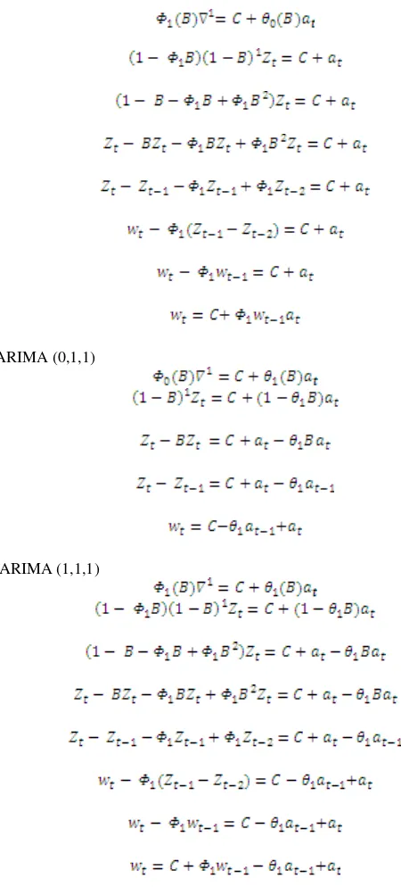
ARIMA (1,1,0)
ARIMA (0,1,1)
ARIMA (1,1,1)
The next steps are to estimate the parameters of the models. The estimation of parameter for ARIMA (1,1,0) model we used software SAS 9.0. The following are the results.
Table 2: The Estimation of Parameter for ARIMA (1,1,0) The ARIMA Procedure
Conditional Least Squares Estimation
Parameter Estimate Error t Value Pr > |t| MU 0.64704 0.17926 3.61 0.0006 AR1,1 0.32177 0.12549 2.56 0.0130
Sept.-Oct
The coefficient value for C is 0,64704 , and t-test=3.61 with p-value=0.0006 and we conclude that C is difference from 0. The estimate for the coefficient of AR(1) is 0,32177 t-test=2.56 with p-value=0.013 which is sifnificant. Therefore the AR(1) in the model is significant. So the estimation of ARIMA (1,1,0) model is:
Based on the estimation above, the parameter AR(1) is significant, so we can used the ARIMA (1,1,0) model to explain the series data.
The estimation of parameter for ARIMA (0,1,1) model we used software SAS 9.0. The following are the results.
Table 3: The Estimation of Parameter for ARIMA (0,1,1)
The ARIMA Procedure Conditional Least Squares Estimation
Parameter Estimate Error t Value Pr > |t| MU 0.65364 0.15920 4.11 0.0001
MA1,1 -0.30006 0.12671 -2.37 0.0213
Constant Estimate 0.653636 Variance Estimate 0.892929 Std Error Estimate 0.944949 AIC 2.779794 BIC 2.886369 Number of Residuals 59
The coefficient value for C is 0,65364 , and t-test=4.11 with p-value=0.0001 and we conclude that C is difference from 0. The estimation for the coefficient of MA(1) is -0.30006 t-test =-2.37 with p-value=0.0213 <0.05 which is significant. Therefore the MA(1) in the model is significant. So the estimation of ARIMA (0,1,1) model is:
Based on the estimation above, the parameter MA(1) is significant, so we can used the ARIMA (0,1,1) model to explain the series data.
The estimation of parameter for ARIMA (1,1,1) model we used software SAS 9.0. The following are the results.
Table 4: The Estimation of Parameter for ARIMA (1,1,1)
The ARIMA Procedure Conditional Least Square Estimation
Parameter Estimate Error t Value Pr > |t| MU 0.64936 0.17534 3.70 0.0005 MA1,1 -0.12574 0.40953 -0.31 0.7599 AR1,1 0.21230 0.40300 0.53 0.6004
Constant Estimate 0.511499 Variance Estimate 0.901528 Std Error Estimate 0.949488 AIC 2.753297 BIC 2.823722 Number of Residuals 59
The coefficient value for C is 0,64936, and t-test=3.70 with p-value=0.0005 and we conclude that C is difference from 0. The estimate for the coefficient of AR(1) is 0,21230 with t-test=0.53 p-value=0.6004 which is nonsignificant. Therefore the AR(1) in the model is not significant. The estimate for the coefficient of MA(1) is -0,12574 with t-test=-0.31 and p-value=0.7599 which is nonsignificant. Therefore the MA(1) in the model is not significant.
The estimation of ARIMA (1,1,1) model is:
Based on the result above the parameters of AR (1) and MA(1) are nonsignificant in the model, therefore the ARIMA (1,1,1) is not a good model to explain the series data.
4. THE MODEL CHECKING
After we estimate the significant and candidate for the best model, namely the model ARIMA (1,1,0) and ARIMA (0,1,1). Next we will test for the residual whether they are satisfied the process white noise and satisfied the homoscedasticity [18].
ARIMA (1,1,0)
Figure 8: Graph of white noiseARIMA (1,1,0)
Hypotheses :
H0 = (residual satisfied the white
noise process).
H1 = (residual is not satisfied the
white noise process).
Figure 8, shows that the bar at lag 0 to lag 15 at the graph of white noiseprocess laid below the significant line. From the graph, the p-value for lag 0 to lag 15 are greater than 0.05. Even the lag 0 and lag 1 the value are close to 1. So the p-values > 0,05, therefore we do not reject the null hypotheses and the residual satisfied the white noise process.
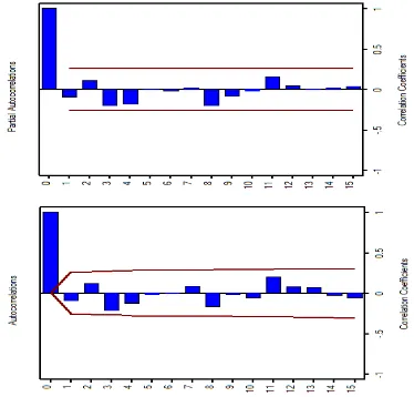
Figure 9: ACF and PACF of residual ARIMA (1,1,0)
Sept.-Oct
in the significant line, therefore we conclude that there is no autocorrelation and the data shows homoscedasticity. The equation of the ARIMA (1,1,0) model satisfied the white noise process and homoscedasticity, therefore the ARIMA (1,1,0) model can be used.
ARIMA (0,1,1)
Figure 10: Graph of white noiseARIMA (0,1,1)
Hypotheses : the white noise process below the significant line. From the graph the p-value at lag 0 to lag 15 laid below the value 0,01, even the p-value lag 0 and lag 1 bar close to 1. Therefore we do not reject the null hypotheses, or the data satisfied the white noise process.
Figure 11: Graph of ACF and PACF residual ARIMA (0,1,1)
In Figure 11 the graph ACF and PACF from the residual ARIMA (0,1,1) model all the bar from lag 1 to lag 15 laid in significant line, therefore there is no autocorrelation and the data satisfied the homoscedasticity.
To compare which one is the best model between ARIMA (1,1,0) and ARIMA (0,1,1), we compare the values of MSE (Mean Square Error), AIC (Akaike Information Criteria), and BIC (Bayesian Information Criteria)[16, 17].
Table 5: The values of MSE, AIC, and BIC ARIMA(1,1,0) is less than the BIC of ARIMA(0,1,1). Based on the values of MSE, AIC and BIC the best model is the model with the smaller values of MSE, AIC and BIC, therefore the best model is the ARIMA (1,1,0).
5. FORECASTING
From the analysis above, we have the best model is ARIMA(1,1,0), the next step is that we are going to use this model for forecasting or prediction for the future six periode. In this forecasting, we will predict the values of CPI from January to June 2014.
Figure 12 below shows the prediction values of CPI Bandar Lampung City from January to June 2014 are increase.
65
(with forecasts and their 95% confidence limits)
Figure 12: Time Series Plot for Forecasting of CPI
Table 6: Forecasting for CPI values from January to June 2014
Month Real Data Forecasting
January
Figure 13: Graph of Real Data and Forecasting of CPI
Sept.-Oct
that the forecasting from the ARIMA (1,1,0) are very good and very close to the real data.
REFERENCES
[1] Monga,G.S.(1977). Mathematics and Statistics for Economics. New Delhi:Vikas Publishing House. [2] Subhani,M.I. and Panjwani,K., (2009). Relationship
between Consumer Price Index (CPI) and Govern-ment Bonds. South Asian Journal of Management Sciences. Vol.3, No.1, pp.11-17.
[3] Mendenhall,W., Reinmuth,J.E., Beaver, R. and Duhan, D. (1986). Statistics for Management and Economics.
Boston: Duxbury Press.
[4] Boskin, M.J.,Ellen R. D., Gordon, R.J., Zvi Griliches and Jorgenson,D.W. (1998). Consumer Prices, the Consumer Price Index, and the Cost of Living. The Journal of Economic Perspectives, Vol. 12, No. 1, pp. 3-26.
[5] Cryer J.D. and Chan K.S. (2008). Time Series Analysis with Application in R. New York :Springer.
[6] Brocwell,P.J., and Davis,R.A. (2002). Introduction to time series and Forecasting. New York: Springer. [7] Box,G.E.P. and Jenkins,G.M. (1976). Time series
Analysis: Forecasting and Control. San Fransisco: Holden-Day.
[8] Montgomery, D.C., Jennings,C.L., and Kulahci,M. (2008). Introduction to Time Series Analysis and Forecasting. New York: John Wiley& Sons.
[9] Chatfield, Chris. (2004). The Analysis of Time Series An Indtroduction Sixth Edition. New York: Chapman & Hall/CRC
[10] Wei, W.S. (2006). Time Series Analysis Univariate and Multivariate Methods Second Edition. Canada: Pearson education Inc.
[11] Box, G.E.P. and G.M. Jenkins, (1970). Time series analysis: Forecasting and control. Holden-Day, San Francisco.
[12] Adam, S.O., Awujola,A., and Alumgudu,A.I., (2014). Modeling Nigeria’s CPI using ARIMA model. Int. Journal of Development and Economic Sustainability,
Vol.2, No2, pp37-47.
[13] Fengwang Zhang, Wengang Che, Beibei Xu, and Jingzhi Xu, (2013). The Research of ARMA Model in CPI Time Series. Proceedings of the 2nd Int. Symposium on Computer, Communi-cation, Control and Automation (ISCCCA).
[14] Pankratz, Alan. (1991). Forecasting with Dynamic Regression Models. Canada:Willey Intersciences Publication.
[15] Tsay, R.S. (2010). .Analysis of Financial Time Series Third Edition. Canada: John Wiley & Son Inc.
[16] Yafee, R. A. Introduction To Time Series Analysis and Forecasting With Applications of SAS and SPSS. New York: Academic Press Inc.
[17] Chair of Statistic. (2011). A First Course on Time Series Analysis. University of Wurzbug.
[18] Shaikh A. Hamid and Tej S. Dhakar. (2008). The behaviour of the US consumer price index 1913–2003: a study of seasonality in the monthly US CPI.