Chp09 – Classical Statistical Inference

Introduction to Probability

SECOND EDITION

Dimitri

P.

Bertsekas and John N. Tsitsiklis

Massachusetts Institute of Technology

WWW site for book information and orders

http://www.athenasc.com

9

Classical Statistical Inference

Contents

9.1. Classical Parameter Estimation .

9.2. Linear Regression . . .

.

9.3. Binary Hypothesis Testing

9.4. Significance Testing .

.

.

9.5. Summary and Discussion

Problems . . .

.

·

p. 460

·

p. 475

·

p. 485

·

p. 495

·

p. 506

·

p. 507

459

The third section deals with binary hypothesis testing problems. Here,

we develop methods that bear similarity with the (Bayesian) MAP method,

discussed in the preceding chapter. In particular, we calculate the "likelihood"

of each hypothesis under the observed data, and we choose a hypothesis by

comparing the ratio of the two likelihoods with a suitably chosen threshold.

The last section addresses different types of hypothesis testing problems.

For an example, suppose a coin is tossed

n

times, the resulting sequence of

heads and tails is observed. and we wish to decide whether the coin is fair or

not . The main hypothesis that we wish to test is whether

p

=

1/2, where

p

denotes the unknown probability of heads. The alternative hypothesis

(p

i= 1 /2)

is

composite,

in the sense that it consists of several, possibly infinitely many,

subhypotheses (e.g. ,

p

=

0. 1 .

p

=

0.4999.

etc . ) . It is clear that no method can

reliably distinguish between a coin with

p

=

0

.

5

and a coin with

p

=

0.4999

on the basis of a moderate number of observations. Such problems are usually

approached using the methodology of

significance testing.

Here, one asks the

question: "are the observed data compatible with the hypothesis that

p

=

0.5?"

Roughly speaking, a hypothesis is rejected if the observed data are unlikely to

have been generated "accidentally" or "by chance." under that hypothesis.

Major Terms, Problems, and Methods in this Chapter

•

Classical statistics

treats unknown parameters as constants to be

determined. A separate probabilistic model is assumed for each pos­

sible value of the unknown parameter.

•

In

parameter estimation,

we want to generate estimates that are

nearly correct under any possible value of the unknown parameter.

•

In

hypothesis testing,

the unknown parameter takes a finite number

m

of values

(

m

> 2), corresponding to competing hypotheses; we want

to choose one of the hypotheses, aiming to achieve a small probability

of error under any of the possible hypotheses.

•

In

significance testing,

we want to accept or reject a single hypoth­

esis, while keeping the probability of false rejection suitably small.

•

Principal classical inference methods in this chapter:

(a)

Maximum likelihood (ML) estimation:

Select the parame­

ter that makes the observed data "most likely," i.e., maximizes

the probability of obtaining the data at hand (Section 9. 1 ) .

(b)

Linear regression:

Find the linear relation that matches best

460 Classical Statistical Inference Chap. 9

(c)

Likelihood ratio test:

Given two hypotheses, select one based

on the ratio of their "likelihoods," so that certain error probabil­

ities are suitably small (Section

9.3) .

(d)

Significance testing:

Given a hypothesis, reject it if and only if

the observed data falls within a certain rejection region. This re­

gion is specially designed to keep the probability of false rejection

below some threshold (Section

9.4) .

9 . 1

CLASSICAL PARAMETER ESTIMATION

In this section. we focus on parameter estimation, using the classical approach

where the parameter

e

is not random. but is rather viewed as an unknown con­

stant. We first introduce some definitions and associated properties of estima­

tors. We then discuss the maximum likelihood estimator. which may be viewed

as the classical counterpart of the Bayesian

MAP

estimator. We finally focus on

the simple but important example of estimating an unknown mean, and possibly

an unknown variance. We also discuss the associated issue of constructing an

interval that contains the unknown parameter with high probability (a " confi­

dence interval" ). The methods that we develop rely heavily on the laws of large

numbers and the central limit theorem (cf. Chapter

5).

Properties of Estimators

Given observations

X

=

(Xl

.

.

.

.

.

Xn). an

estimator

is a random variable of

the form

8 =

g(X),

for some function

g.

Note that since the distribution of

X

depends on

e.

the same is true for the distribution of 8. We use the term

estimate

to refer to an actual realized value of 8.

Sometimes, particularly when we are interested in the role of the number

of observations

n,

we use the notation 8n for an estimator. It is then also

appropriate to view 8n as a sequence of estimators (one for each value of

n

)

.

The mean and variance of en are denoted Et/J8n] and vart/(8n), respectively.

and are defined in the usual way. Both Et/ [en] and vart/(8n) are numerical

functions of

e.

but for simplicity. when the context is clear we sometimes do not

show this dependence.

We introduce some terminology related to various properties of estimators.

Terminology Regarding Estimators

Let 8n be an

estimator

of an unknown parameter

e,

that is, a function of

Sec. 9. 1 Classical Parameter Estimation 461

•

The

estimation error,

denoted by

e

n , is defined by

e

n

=

e

n

- e.

•

The

bias

of the estimator, denoted by be

(e

n

)

, is the expected value

of the estimation error:

•

The expected value, the variance, and the bias of

e

n depend on

e,

while the estimation error depends in addition on the observations

Xl , . . . ,Xn.

•

We call

e

n

unbiased

if Ee

[e

n

]

= e,

for every possible value of

e.

•

We call

e

n

asymptotically unbiased

if limn-->oo Ee

[e

n

]

= e,

for

every possible value of

e.

•

We call

e

n

consistent

if the sequence

e

n converges to the true value

of the parameter

e,

in probability, for every possible value of

e.

An estimator, being a function of the random observations. cannot be ex­

pected to be exactly equal to the unknown value (). Thus, the estimation error

will be generically nonzero. On the other hand, if the average estimation error

is zero. for every possible value of

e,

then we have an unbiased estimator, and

this is a desirable property. Asymptotic unbiasedness only requires that the es­

timator become unbiased as the number

n

of observations increases. and this is

desirable when

n

is large.

Besides the bias be

_(e

n

)

, we are usually interested in the size of the estima­

tion error. This is captured by the mean squared error Ee

[e�]

. which is related

to the bias and the variance of

e

n according to the following formula:

t

Ee

[8�]

=

b

� (e

n

)

+

vare (

e

ll

)

.

This formula is important because in many statistical problems. t here is a trade­

off between the two terms on the right-hand-side. Often

a

r('duction in the

variance is accompanied by an increase in the bias. Of course. a good estimator

is one that manages to keep both terms small.

We will now discuss some specific estimation approaches. starting with

maximum likelihood estimation. This is a general method that bears similarity

to MAP estimation. introduced in the context of Bayesian inference. We will

subsequently consider the simple but important case of estimating the mean

and variance of a random variable. This will bring about a connection with our

discussion of the laws of large numbers in Chapter

5.

, . . . , Xn ;

to

if IS as

x

9.2. X is () takes

one of the _m values G iven the value of the observation _{X Xl} the values of the l i keli hood function _{p X} Ot ) become avail able for all _il and a value of () tha.t m aximizes _{p X} is selected.

, . . . ! Xl1 ;

0)

=

to

n

i ::::: 1

9

conve-" . . Xn ;

Sec. 9. 1 Classical Parameter Estimation 463

over

O.

When X is continuous, there is a similar possibility, with PMFs replaced

by PDFs: we maximize over 0 the expression

n n

i=l i=l

The term "likelihood" needs to be interpreted properly. In particular, hav­

ing observed the value

x

of X,

px (x;

0

)

is not

the probability that the unknown

parameter is equal to

O.

Instead, it is the probability that the observed value

x

can arise when the parameter is equal to

O.

Thus, in maximizing the likelihood,

we are asking the question: "What is the value of 0 under which the observations

we have seen are most likely to arise?"

Recall that in Bayesian MAP estimation, the estimate is chosen to maxi­

mize the expression

pe (O) px l e (x I

0

)

over all 0, where

pe (O)

is the prior PMF

of an unknown discrete parameter

O.

Thus, if we view

px (x;

0

)

as a conditional

PMF, we may interpret ML estimation as MAP estimation with a

flat prior,

i.e., a prior which is the same for all 0, indicating the absence of any useful

prior knowledge. Similarly, in the case of continuous 0 with a bounded range

of possible values, we may interpret ML estimation as MAP estimation with a

uniform prior:

le (O) c

for all 0 and some constant

c.

Example 9.1. Let us revisit Example 8.2, in which Juliet is always late by an amount X that is uniformly distributed over the interval

[0, 0] , and 0 is an unknown

parameter. In that example. we used a random variable

e

with flat prior PDF

1e (0)

(uniform over the interval

[0, 1])

to model the parameter. and we showed that the MAP estimate is the value x of X. In the classical context of this section, there is no prior, and

0 is treated as a constant, but the ML estimate is also

tJ =

x.

Example 9.2. Estimating the Mean of a Bernoulli Random Variable. We want to estimate the probability of heads, 0, of a biased coin, based on the outcomes of

n

_{independent tosses Xl , " . . Xn (Xi} = 1 for a head, and Xi = ° for a tail). This is similar to the Bayesian setting of Example 8.8, where we assumed a flat prior. We found there that the peak of the posterior PDF (the MAP estimate) is located at

0

=

kin,

where

k

is the number of heads observed. It follows that

kin

is also the ML estimate of 0, so that the ML estimator is

A . . . +

n

This estimator is unbiased. It is also consistent, because

en

converges to

0

in probability, by the weak law of large numbers.

464 Cla.ssical Statistical Inference Chap. 9

Example

9.3.

Estimating the Parameter of an Exponential Random Vari­

able.

Customers arrive to a facility, with the ith customer arriving at time Yi . We assume that the ith interarrival time,

Xi

= Yi - Yi-l (with the convention

Yo

=

0)

is exponentially distributed with unknown parameter

()

,

and that the random vari­ ables

Xl ,

.

.

.

, Xn

are independent. (This is the Poisson arrivals model, studied in Chapter

6.)

We wish to estimate the value of () (interpreted as the arrival rate), on the basis of the observations

XI , . . . , X

n.

The corresponding likelihood function is

n

n

t=1

i=1

and the log-likelihood function is

log

Ix

(x;

0)

₌

n

log

() - OYn,

where

_n

Yn

=

L Xi.

i=1

The derivative with respect to () is

(n/())

-

_Yn,

and by setting it to

0,

we see that the maximum of log

Ix

(x;

0), over 0

� 0,

is attained at

_On

=

n/Yn.

The resulting estimator is

�

(Yn ) -1

8n =

-

_n

It is the inverse of the sample mean of the interarrival times, and it can be inter­ preted as an empirical arrival rate.

Note that by the weak law of large numbers,

_Yn/n

converges in probability to

E

[

Xt

l

=

I/O,

as

n

-+

oc. This can be used to show that

en

converges to () in probability, so the estimator is consistent.

Our discussion and examples so far have focused on the case of a single

unknown parameter (). The next example involves a two-dimensional parameter.

Example

9.4.

Estimating the Mean and Variance of a Normal.

Consider the problem of estimating the mean

JL

and variance

_v

of a normal distribution using

n

independent observations

XI , . . . , X

_n.

The parameter vector here is

()

=

(JL,

v).

The corresponding likelihood function is

After some calculation it can be written as t

1

{

ns�

} {

n

(

mn - JL

)

2

}

Sec. 9. 1 Classical Parameter Estimation

where

mn

is the realized value of the random variable

n

Mn

=

� LXl'

i=l

and 8

�

is the realized value of the random variable

The log-likelihood function is

n n n8

�

n

(

mn

- J-l)2

10g fx(x; J-l, v)

=

-"2

· log(2rr)

- "2

.

log v

-2v -

2v

465

Setting to zero the derivatives of this function with respect to

_J-l

and v, we obtain the estimate and estimator, respectively,

Note that

Mn

is the sample mean, while

S!

may be viewed as a "sample variance." As will be shown shortly,

E9[S�l

converges to

_v

as n increases, so that

S�

is asymp­

totically unbiased. Using also the weak law of large numbers, it can be shown that

Mn

and

S�

are consistent estimators of

_J-l

and v, respectively.

Maximum likelihood estimation has sOAme appealing properties. For exam­

ple, it obeys the

invariance principle:

if

en

is the ML estimate of 0, then for

any one-to-one function

h

of 0, the

1\IL

estimate of the parameter (

=

h(O)

is

h(en).

Also. when the observations are Li.d . , and under some mild additional

assumptions, it can be shown that the ML estimator is consistent .

Another interesting property is that when 0 is a scalar parameter, then

under some mild conditions, the ML estimator has an

asymptotic normality

property. In particular. it can be shown that the distribution of

(en - O)/a(en),

where

a2(en )

is the variance of

en ,

approaches a standard normal distribution.

Thus, if we are able

to a

l

s

o

estimate a(8n),

we can use it to derive an error vari­

ance estimate based on a normal approximation. When 0 is a vector parameter,

a similar statement applies to each one of its components.

t To verify this. write for

i

=

1,

... , n,

sum over

i,

and note that

n

n

466 Classical Statistical Inference Chap. 9

Maximum Likelihood Estimation

•

We are given the realization

x =

(Xl,

..

.

, Xn )

of a random vector

X

=

(Xl , . . . , Xn ) ,

distributed according to a

PMF PX(Xj

e)

or PDF

!x(Xj

e).

•

The maximum likelihood (ML) estimate is a value of

e

that maximizes

the likelihood function,

px (x; e)

or

fx (x; e),

over all

e.

•

The ML estimate of a one-to-one function

h(e)

of

e

is

h(en),

where

en

is the ML estimate of

e

(

the invariance principle

)

.

•

When the random variables

Xi

are i.i.d., and under some mild addi­

tional assumptions, each component of the ML estimator is consistent

and asymptotically normal.

Estimation of the Mean and Variance of a Random Variable

We now discuss the simple but important problem of estimating the mean and

the variance of a probability distribution. This is similar to the preceding Exam­

ple 9.4, but in contrast with that example, we do not assume that the distribution

is normal. In fact, the estimators presented here do not require knowledge of the

distributions

px (x; e)

[

or

fx (x; e)

if

x

is continuous

]

.

The sample mean is not necessarily thAe estimator with the smallest vari­

ance. For example, consider the estimator

en

= O.

which ignores the observa­

tions and always yields an estimate of zero. The variance of

e

n is zero, but its

bias is bo

(e

n

)

= -e.

In particular, the mean squared error depends on

e

and is

equal to

e2.

The next example compares the sample mean with a Bayesian MAP esti­

mator that we derived in Section

8.2

under certain assumptions.

Sec. 9. 1 Classical Parameter Estimation 467

(). For the case where the prior mean of () was zero, we arrived at the following estimator:

A

Xl + . . . + Xn

en

= .

n + l

This estimator is biased, because _{El den]} =

n()/(n + 1)

and b9

(

e

n

)

=

-()/(n + 1).

However, limn_a;) b9

(

e

n

)

=

0, so en is asymptotically unbiased. Its variance is

and it is slightly smaller than the variance

v/n

of the sample mean. Note that in the special case of this example, var9

(

e

n

)

is independent of (). The mean squared error is equal to

Suppose that in addition to the sample mean/estimator of (),

Xl + · · · + Xn

Mn = _n

,

we are interested in an estimator of the variance

v.

A

natural one is

which coincides with the ML estimator derived in Example

9.4

under a normality

assumption.

U sing the facts

we have

E(9,v)

[xl] =

()2

+ V,

E(e,")

[

s!]

=

!

E(e,")

[t.

Xl -

2Mn t.

Xi + nM�

1

=

_E(e,")

[

!

t

Xl - 2M� + M�

]

=

E(9,v)

[� t

Xl - M�

]

1=1

=

()2

+ V -

(()2

+

�)

n - l

468 Classical Statistical Inference Chap. 9

Thus,

S�

is not an unbiased estimator of

v,

although it

is

asymptotically unbi­

ased.

We can obtain an unbiased variance estimator after some suitable scaling.

This is the estimator

n

�2

1

_L

n

-2

Sn = --

(Xi

- Aln)2

=

--Sn.

n - l

_i=l

n - l

The preceding calculation shows that

E(8,v)

[S�]

=

v,

so

_�

S�

is an unbiased estimator of

v,

for all n. However. for large n, the estimators

-2

S

�

and

Sn

are essentially the same.

Estimates of the Mean and Variance of a Random Variable

Let the observations

_{Xl , . . . , Xn}

be i.i.d., with mean (J and variance

v

that

are unknown.

•

The sample mean

Xl + " ' + Xn Atfn

=

_n

is an unbiased estimator of (J, and its mean squared error is

vln.

•

Two variance estimators are

n

S�

=

n I l

L(Xi - Mn)2. _i=l

•

The estimator

S�

coincides with the ML estimator if the

Xi

are nor­

mal. It is biased but asymptotically unbiased. The estimator

S�

is

unbiased. For large

n,

the two variance estimators essentially coincide.

Confidence Intervals

Consider an estimator

en

of an unknown parameter (J. Besides the numerical

value provided by an estimate. we are often interested in constructing a so-called

confidence interval. Roughly speaking, this is an interval that contains (J with a

certain high probability, for every possible value of (J.

For a precise definition, let us first fix a desired

confidence level,

1

- Q,

Sec. 9. 1 Classical Parameter Estimation 469

a lower estimator

8;;-

and an upper estimator

8;t" ,

designed so that

8;;- ::; 8;t" ,

and

for every possible value of (). Note that, similar to estimators,

8;;-

and

8;t' ,

are

functions of the observations, and hence random variables whose distributions

depend on

e.

We call

[8;;- ,

8;i]

a

1

-

Q

confidence interval.

Example 9.6. Suppose that the observations Xi are LLd. normal, with unknown

mean () and known variance

v.

Then, the sample mean estimator

is normal,t with mean () and variance

v/n.

Let

Q

=

0.05.

Using the CDF

4>(z)

of the standard normal (available in the normal tables), we have

4>(1.96)

=

0.975

=

l - Q/2

and we obtain

P9

(len -

()I

::;

1.96

)

=

0

.

95

.

Nn

We can rewrite this statement in the form

which implies that

[A

en -

en

A

₊

is a

95%

confidence intervaL where we identify

e�

and

e�

with

en -

l.96

Nn

and

en

+

1.96

respectively.

In the preceding example, we may be tempted to describe the concept of

a

95%

confidence interval by a statement such

as

"the true parameter lies in

the confidence interval with probability

0.95."

Such statements, however, can

be ambiguous. For example, suppose that after the observations are obtained,

the confidence interval turns out to be

[-2.3, 4. 1] .

We cannot say that

e

lies in

[-2.3, 4.1]

with probability

0.95,

because the latter statement does not involve

any random variables; after all, in the classical approach,

e

is a constant. In­

stead, the random entity in the phrase "the true parameter lies in the confidence

interval" is the confidence interval, not the true parameter.

For a concrete interpretation, suppose that () is fixed. We construct a

confidence interval many times, using the same statistical procedure, i.e., each

470 Classical Statistical Inference Chap. 9

time, we obtain an independent collection of

n

observations and construct the

corresponding

95%

confidence interval. We then expect that about

95%

of these

confidence intervals will include (). This should be true regardless of what the

value of () is.

Confidence Intervals

•

A

confidence interval

for a scalar unknown parameter () is an interval

whose endpoints

8;;

and

et

bracket () with a given high probability.

• 8;;

and

at

are random variables that depend on the observations

Xl , . . . ,Xn.

•

A 1

- 0:

confidence interval is one that satisfies

for all possible values of ().

Confidence intervals are usually constructed by forming an interval around

an estimator

8

n

(

cf. Example

9.6).

Furthermore, out of a variety of possible

confidence intervals, one with the smallest possible width is usually desirable.

However, this construction is sometimes hard because the distribution of the

error

8

_{n :- () is either unknown or depends on (). Fortunately, for many important}

models,

en -

() is asymptotically normal and asymptotically unbiased. By this

we mean that the CDF of the random variable

en -

()

vare

(

e

n

)

approaches the standard normal CDF as

n

increases, for every value of (). We may

then proceed exactly as in our earlier normal example

(

Example

9.6),

provided

that vare

(

8

n

)

is known or can be approximated, as we now discuss.

Confidence Intervals Based on Estimator Variance Approximati�ns

Suppose that the observations

_Xi

are i.i.d. with mean () and variance

v

that are

unknown. We may estimate () with the sample mean

A X1 + .. . + Xn

n

and estimate

v

with the unbiased estimator

n

A

I

L

A

Sec. 9. 1 Classical Parameter Estimation 471

that we introduced earlier. In particular, we may estimate the variance

v / n

of

the sample mean by

S�/n.

Then, for a given

0,

we may use these estimates

and the central limit theorem to construct an (approximate)

1

-

0

confidence

interval. This is the interval

where

z

is obtained from the relation

o

�(z) = l

-2

and the normal tables, and where

S

n

is the positive square root of

S� .

For

instance, if

0

=

0.05, we use the fact

� ( 1 .96)

=

0.975

=

1

-

0/2

(from the

normal tables) and obtain an approximate 95% confidence interval of the form

Note that in this ?pproach, there are two different approximations in effect.

First, we are treating

en

as if it were a normal random variable; second, we are

replacing the true variance

v/n

of

en

by its estimate

S�/n.

Even in the special case where the

Xi

are normal random variables, the

confidence interval produced by the preceding procedure is still approximate.

The reason is that

S�

is only an approximation to the true variance

v,

and the

random variable

yn

(en - 8)

Tn

=

�

Sn

is not normal. However, for normal

Xi,

it can be shown that the PDF of

Tn

does not depend on

8

and

v,

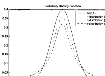
and can be computed explicitly. It is called the

t-distribution with

n

-

1

degrees of freedom.

t

Like the standard normal

PDF, it is symmetric and bell-shaped, but it is a little more spread out and has

heavier tails (see Fig.

9.3).

The probabilities of various intervals of interest are

available in tables, similar to the normal tables. Thus, when the

Xi

are normal

(or nearly normal) and

n

is relatively small, a more accurate confidence interval

is of the form

472 Classical Statistical Inference Chap. 9

where

z

is obtained from the relation

and Wn- l (Z) is the

CDF

of the t-distribution with

n -

1

degrees of freedom,

available in tables. These tables may be found in many sources. An abbreviated

version is given in the opposite page.

0.35

0.3

0.25

0.2

0.1 5 0. 1 0.05

-: .:: ::::

Probability Density Function

--N(O, l )

t-distribution (n::l l ) - - t-distribution (n=3) - - - t-distribution (n::2)

...

.:::: =. .::::

--5 -4 -3 -2 -1 o 2 3 4 5

Figure 9.3. The PDF of the t-distribution with n - 1 degrees of freedom in comparison with the standard normal PDF.

On the other hand, when

n

is moderately large (e.g.,

n �

50), the t­

distribution is very close to the normal distribution, and the normal tables can

be used.

Example 9.7. The weight of an object is measured eight times using an electronic scale that reports the true weight plus a random error that is normally distributed with zero mean and unknown variance. Assume that the errors in the observations are independent. The following results are obtained:

0.5547, 0.5404, 0.6364, 0.6438, 0.4917, 0.5674, 0.5564, 0.6066.

We compute a

95%

confidence interval

(

a =

0.05)

using the t-distribution. The value of the sample mean _en is

0.5747,

and the estimated variance of _en is

�2 n

Sn ₌

1

_(Xi _ 8n)2 ₌

3.2952 . 10-4 •

Sec. 9. 1 Classical Parameter Estimation 473

474 Classical Statistical Inference Chap. 9

The approximate confidence intervals constructed so far relied on the par­

ticular estimator

S�

for the unknown variance

v.

However, different estimators

or approximations of the variance are possible. For example, suppose that the

observations

Xl , . . . , X n

are Li.d. Bernoulli with unknown mean

8,

and vari­

anc�

v = 8(1 -

8).

Then, instead of

S�A'

the variance could be approximated

by

en( 1 - en).

Indeed, as

n

_increases,

en

_{converges to}

8,

_{in probability, from}

which it can be shown that

en( 1 - en)

converges to

v.

Another possibility is to

just observe that

8(1 - 8)

<

1/4

for all

8

E

[0. 1] ' and use

1 /4

as a conservative

estimate of the variance. The following example illustrates these alternatives.

Example 9.8. Polling. Consider the polling problem of Section

5.4

(Example

5.11),

where we wish to estimate the fraction e of voters who support a particular

candidate for office. We collect n independent sample voter responses

Xl , . . . , X

n,

where

Xi

is viewed as a Bernoulli random variable. with

Xi

=

1

if the ith voter sup­ ports the candidate. We estimate e with the sample mean

en,

and construct a con­

fidence interval based on a normal approximation and different ways of estimating or approximating the unknown variance. For concreteness, suppose that

684

out of a sample of n =

1200

voters support the candidate, so that

en

=

684/1200

=

0.57.

(a) If we use the variance estimate

=

(

684 .

(

1 -

2

+

( 1200 - 684) .

(

0

_

2)

;::: 0.245,

and treat

en

as a normal random variable with mean e and variance

0.245,

we obtain the

95%

confidence interval

[

en

-

1.96

en

+

1.96

1

=

[

0.57 - 1.96 ·

v'll.245,

0.57

+

=

[0.542, 0.598].

(b) The variance estimate

A A

684

(

684

₎

en ( 1 - e

n

)

=

1200 ' 1 - 1200

=

0.245

is the same as the previous one (up to three decimal place accuracy), and the resulting

95%

confidence interval

[

8n

-

1.96

en) , en

+

1 .96

en)

1

Sec. 9.2 Linear Regression 475

(c) The conservative upper bound of

1/4

for the variance results in the confidence interval

[en

- 1.96

en

+

1.96

=

[

0.57 -

0.57

+

1200

1200

=

[0.542, 0.599],

which is only slightly wider, but practically the same as before.

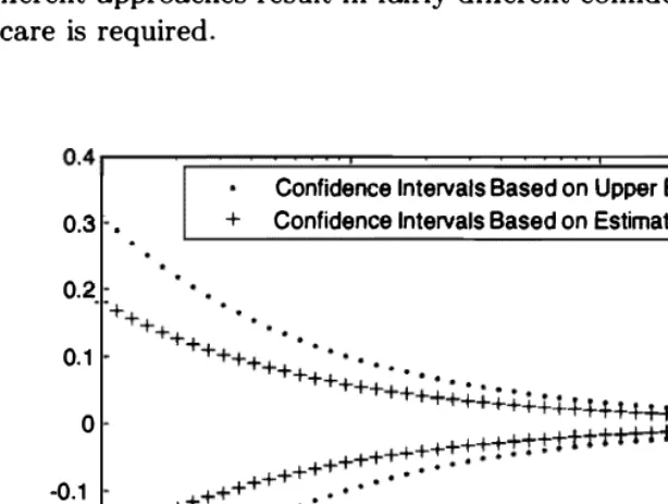
Figure

9.4

illustrates the confidence intervals obtained using methods (b) and (c), for a fixed value _en =

0.57

and a range of sample sizes from n =

10

to

n

10,000.

We see that when n is in the hundreds, as is typically the case in

voter polling, the difference is slight. On the other hand, for small values of n,

the different approaches result in fairly different confidence intervals, and therefore some care is required.

Confidence Intervals Based on Upper Bound

0.3 •

0.2

0.1

o -0.1

-0.2

-0.3 •

+ Confidence Intervals Based on Estimated Variance

1� 1� 1� 1�

n

Figure 9.4. The distance of the confidence interval endpoints from

en

for meth­ ods (b) and (c) of approximating the variance in the polling Example 9.8, when en = 0.57 and for a range of sample sizes from n = 10 to n = 10,000.

9.2 LINEAR REGRESSION

9

in the context of various probabilistic frameworks, which provide perspective and

a for

first consider the case of only two

wish to model between two

a

a systematic , approximately linear relation between Xi and Yi . Then, it

is

natural

to to build

a

where _()o In

the value

difference

ove

r

fh

are

unknown parameters to be est imated .

given

some

00

{)

1 of

to Xi 1 as predicted by the is

A choice

a good to

the

parameter estimates 00

residuals.

n n

- ili )2 = -

(JO

-

(JI X

z

)2

,

i= 1 i = 1

: see Fig. for

an illustration.

o

9.5: Ill ustration of a set of d ata

small residuals motivation, the

{h

minimize

x

OO +81 X, obtained by over Yi),

and a linear model Y =

t he sum of the squares of the residuals

-Sec. 9.2 Linear Regression 477

Note that the postulated linear model may or may not be true. For exam­

ple, the true relation between the two variables may be nonlinear. The linear

least squares approach aims at finding the best possible linear model. and in­

volves an implicit hypothesis that a linear model is valid. In practice, there is

often an additional phase where we examine whether the hypothesis of a linear

model is supported by the data and try to validate the estimated �model.

�

To derive the formulas for the linear regression estimates

(}o

and

(}1 ,

we

observe that once the data are given, the sum of the squared residuals is a

quadratic function of

(}o

and

(}1.

To perform the minimization, we set to zero the

partial derivatives with respect to

(}o

and (}l . We obtain two linear equations in

(}o

and

(}l ,

which can be solved explicitly. After some algebra, we find that the

solution has a simple and appealing form, summarized below.

Linear Regression

Given

n

data pairs

(Xi, Yi),

the estimates that minimize the sum of the

squared residuals are given by

where

n

I)Xi - X)(Yi

- y)

{it

=

i=l

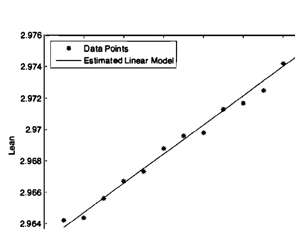
n

Example

9.9. The leaning tower of Pisa continuously tilts over time. Measure­

ments between years

1975

and

1987

of the "lean" of a fixed point on the tower (the distance in meters of the actual position of the point, and its position if the tower were straight) have produced the following table.

Year

1975 1976 1977 1978 1979 1980 1981

Lean

2.9642 2.9644 2.9656 2.9667 2.9673 2.9688 2.9696

Year

1982 1983 1984 1985 1986 1987

Lean

2.9698 2.9713 2.9717 2.9725 2.9742 2.9757

478 Classical Statistical Inference

and is illustrated in Figure 9.6.

*

Justification of the Least Squares Formulation

t

The least squares formulation can be justified on the basis of probabilistic con­

siderations in several different ways, based on different sets of assumptions.

(a)

Maximum likelihood

(

linear model, normal noise

)

.

We assume that

the

Xi

are given numbers (not random variables) . We assume that

_Yi

is the

Sec. 9.2 Linear Regression 479

realization of a random variable

Yi,

generated according to a model of the

form

i

=

1 ,

. . .

, n,

where the

Wi

are i.i.d. normal random variables with mean zero and vari­

ance

(72.

It follows that the

Yi

are independent normal variables, where

Yi

has mean

(}

o

+

(}lXi

and variance

(72.

The likelihood function takes the form

f

y

( ' (}) = IIn

y,

1

exp

{ _

(Yi - (}O - (}lXi)2 }

2

2

.

i=l

(7

Maximizing the likelihood function is the same as maximizing the exponent

in the above expression, which is equivalent to minimizing the sum of the

squared residuals. Thus, the linear regression estimates can be viewed as

ML estimates within a suitable linear Inormal context. In fact they can be

shown to be unbiased estimates in this context. Furthermore, the variances

of the estimates can be calculated using convenient formulas (see the end­

of-chapter problems) , and then used to construct confidence intervals using

the methodology of Section

9. 1 .

(b)

Approximate Bayesian linear LMS estimation (under a possibly

nonlinear model).

Suppose now that both

Xi

and

Yi

are realizations of

random variables Xi and

Yi.

The different pairs

(

X

i

,

Yi)

are Li.d., but

with unknown joint distribution. Consider an additional independent pair

(Xo, Yo),

with the same joint distribution. Suppose we observe

Xo

and

stituting these estimates into the above formulas for (}o and

(}1,

we recover

the expressions for the linear regression parameter estimates given earlier.

Note that this argument does not assume that a linear model is valid.

(c)

Approximate Bayesian LMS estimation (linear model).

Let the

pairs

(Xi,

Yi)

be random and i.i.d. as in (b) above. Let us also make the

additional assumption that the pairs satisfy a linear model of the form

Yi

=

(}

o

+

(}lXi

+

Wi,

480 Classical Statistical Inference Chap. 9

E[Yo

I

Xol

minimizes the mean squared estimation error

E[(Yo - g(XO))2] ,

over all functions

g.

Under our assumptions,

E[Yo

I

Xol

=

0

0

+OlXO.

Thus,

the true parameters 00 and

fh

minimize

over all O

h

and

Oi.

By the weak law of large numbers, this expression is the

limit as

n ---t 00

of

This indicates that we will obtain a good approximation of the minimizers

of

E[(Yo - Oh - OiXO)2]

(

the true parameters

)

, by minimizing the above

expression

(

with

Xi

and

Yi

replaced by their observed values

Xi

and

Yi,

respectively

)

. But minimizing this expression is the same as minimizing

the sum of the squared residuals.

Bayesian Linear Regression

t

Linear models and regression are not exclusively tied to classical inference meth­

ods. They can also be studied within a Bayesian framework, as we now explain.

In particular, we may model

Xl, .. . ,Xn

as given numbers, and Yl , . . . ,Yn as the

observed values of a vector

Y

=

(Yl, " " Yn)

of random variables that obey a

linear relation

Here,

8 = (80 , 81 )

is the parameter to be estimated, and

WI , .

.

.

, �Vn

are Li.d.

random variables with mean zero and known variance

(12.

Consistent with the

Bayesian philosophy, we model

80

and

8 1

as random variables. We assume

that

80, 81 , WI .

.

.

. , Wn

are independent, and that

80. 8 1

have mean zero and

variances

(15, (1r.

respectively.

We may now derive a Bayesian estimator based on the MAP approach and

the assumption that

80, 81 ,

and

WI , . ..

, Wn

are normal random variables. We

maximize over

00, 01

the posterior PDF

ielY(Oo,

01 I

Y! , .

.

.

, Yn)'

By Bayes' rule,

the posterior PDF is

+

divided by a positive normalizing constant that does not depend on

(Oo,Od.

Under our normality assumptions, this expression can be written as

{ 05 } { Or } lIn { (Yi - 00 - XiOi)2 }

c · exp -

-

· exp -

-

.

exp -

_,

2(12

_o

2(12

1

i=l

2(12

t This subsection can be skipped without loss of continuity.

Sec. 9.2 Linear Regression 481

where

c

is a normalizing constant that does not depend on

(00. OJ ).

Equivalently,

we minimize over

00

and

01

the expression

Note the similarity with the expression

L�l

(Yi - 00

_{-xiOl )2,}

_{which is minimized}

in the earlier classical linear regression formulation. (The two minimizations

would be identical if

ao

and

al

were so large that the terms

OS/2a5

and

8I/2aI

could be neglected. ) The minimization is carried out by setting to zero the

partial derivatives with respect to

80

and

81 .

After some algebra, we obtain the

following solution.

Bayesian Linear Regression

•

Model:

(a) We assume a linear relation

Yi

= 80 + 81xi + Wi .

(b) The

Xi

are modeled as known constants.

(c) The random variables

80, 8 1 , WI , . . . , Wn

are normal and inde­

pendent.

(d) The random variables

80

and

81

have mean zero and variances

a5, aI,

respectively.

(e) The random variables

Wi

have mean zero and variance

a2 •

•

Estimation Formulas:

Given the data pairs

(Xi, Yi),

the

MAP

estimates of

80

and

81

are

where

i=l

2

A

nao

_ A _

80

= _{2 2}

(y

-

81x),

a

+

nao

1

n

482 Classical Statistical Inference Chap. 9

We make a few remarks:

(a) If

0'2

is very large compared to

0'5

and

O'

r

,

we obtain

Bo

�

0

and

Bl

� o.

What is happening here is that the observations are too noisy and are

essentially ignored, so that the estimates become the same as the prior

means, which we assumed to be zero.

(b) If we let the prior variances

0'5

and

O'

r

increase to infinity, we are indicating

the absence of any useful prior information on 80 and

81.

In this case,

the MAP estimates become independent of

0'2,

and they agree with the

classical linear regression formulas that we derived earlier.

(c) Suppose, for simplicity, that

x = O.

When estimating

81 ,

the values

Yi

of

the observations

Yi

are weighted in proportion to the associated values

Xi.

This is intuitive: when

Xi

is large, the contribution of

81xi

to

Yi

is relatively

large, and therefore

Yi

contains useful information on

81 .

Conversely, if

Xi

is zero, the observation

Yi

is independent of 81 and can be ignored.

A A

(d) The estimates

()o

and

()1

are linear functions of the

Yi,

but not of the

Xi .

Recall, however, that the

Xi

are treated as exogenous, non-random quanti­

ties, whereas the

Yi

are observed values of the random variables

Yi.

Thus

the MAP estimators

80, 8 1

are linear estimators, in the sense defined in

Section

8.4.

_{It follows, in view of our normality assumptions, that the esti­}

mators are also Bayesian linear LMS estimators as well as LMS estimators

(cf. the discussion near the end of Section

8.4).

Multiple Linear Regression

Our discussion of linear regression so far involved a single

explanatory vari­

able,

namely

X,

a special case known as

simple regression.

The objective was

to build a model that explains the observed values

Yi

on the basis of the val­

ues

Xi.

Many phenomena, however, involve multiple underlying or explanatory

variables. (For example, we may consider a model that tries to explain annual

income as a function of both age and years of education.) Models of this type

are called

multiple regression

models.

For instance, suppose that our data consist of triples of the form

(Xi , Yi, Zi)

and that we wish to estimate the parameters

()j

of a model of the form

As an example,

Yi

may be the income,

Xi

the age, and

Zi

the years of education

of the ith person in a random sample. We then seek to minimize the sum of the

squared residuals

n

L(Yi

-

()o

- ()lXi - ()2Zi)2,

i=1

Sec. 9.2 Linear Regression 483

Oi

is conceptually the same as for the case of a single explanatory variable, but

of course the formulas are more complicated.

As a special case, suppose that

Zi

=

XT ,

in which case we are dealing with

a model of the form

Y

�

00

+

OI X

+

02x2.

Such a model would be appropriate if there are good reasons to expect a quadratic

dependence of

Yi

on

Xi.

(

Of course, higher order polynomial models are also pos­

sible.

)

While such a quadratic dependence is nonlinear, the underlying model is

still said to be linear, in the sense that the unknown parameters

OJ

are linearly

related to the observed random variables

Yi .

More generally, we may consider a

model of the form

_m

Y

�

00

+

L Ojhj (x),

j=1

where the

hj

are functions that capture the general form of the anticipated de­

pendence of y on

x.

We may then obtain parameters

00, 01 ,

. . .

, Om

by minimizing

over

00, 01 , . . . ,Om

the expression

This minimization problem is known to admit closed form

as

well as efficient

numerical solutions.

Nonlinear Regression

There are nonlinear extensions of the linear regression methodology to situations

where the assumed model structure is nonlinear in the unknown parameters. In

particular, we assume that the variables

x

and

Y

obey a relation of the form

Y

�

h(x; 0),

where

h

is a given function and

0

is a parameter to be estimated. We are given

data pairs

(Xi, Yi),

i

=

1,

. .

.

, n,

and we seek a value of

0

that minimizes the sum

of the squared residuals

n

L (Yi - h(Xi ; 0)) 2.

i=l

484 Classical Statistical Inference Chap. 9

where the

Wi

are Li.d. normal random variables with zero mean. To see this,

note that the likelihood function takes the form

f

y

( ·e)

Y,

=

rrn

1

exp

{ _

(Yi - h(Xi; e))2 }

2 2

'

i=l

0"

where

0"2

is the variance of

Wi.

Maximizing the likelihood function is the same

as maximizing the exponent in the above expression, which is equivalent to

minimizing the sum of the squared residuals.

Practical Considerations

Regression is used widely in many contexts, from engineering to the social sci­

ences. Yet its application often requires caution. We discuss here some important

issues that need to be kept in mind, and the main ways in which regression may

fail to produce reliable estimates.

(a)

Heteroskedasticity.

The motivation of linear regression as ML estima­

tion in the presence of normal noise terms

Wi

contains the assumption that

the variance of

Wi

is the same for all

i.

Quite often, however, the variance

of

Wi

varies substantially over the data pairs. For example, the variance of

Wi

may be strongly affected by the value of

Xi.

(For a concrete example,

suppose that

Xi

is yearly income and

Yi

is yearly consumption. It is natural

to expect that the variance of the consumption of rich individuals is much

larger than that of poorer individuals. ) In this ca..c;;e, a few noise terms with

large variance may end up having an undue influence on the parameter

estimates. An appropriate remedy is to consider a weighted least squares

criterion of the form

2:�1 ();i(Yi eo e1xi)2,

where the weights

();i

are

smaller for those

i

for which the variance of

Wi

is large.

(b)

Nonlinearity.

Often a variable

X

can explain the values of a variable

y,

but the effect is nonlinear. As already discussed, a regression model

based on data pairs of the form

(h(Xi), Yi)

may be more appropriate, with

a suitably chosen function

h.

(c)

Multicollinearity.

Suppose that we use two explanatory variables

X

and

z

in a model that predicts another variable

y.

If the two variables

x

and

z

bear

a strong relation, the estimation procedure may be unable to distinguish

reliably the relative effects of each explanatory variable. For an extreme

example, suppose that the true relation is of the form

Y

=

2x

+ 1

and that

the relation

z =

2x

always holds. Then� the model

Y

= z + 1

is equally .valid,

and no estimation procedure can discriminate between these two models.

(d)

Overfitting.

Multiple regression with a large number of explanatory vari­

to a

suIting provide a

nevertheless be incorrect. As a rule of thumb, there ten times

)

more data

(e) a two x

y should not be mistaken for a discovery a causal relation. A tight

x has a causal on y� but

be some

Xi be

child and Yi be the wealth of the second child in the same family.

We expect to increase roughly linearly with X i , but this can be traced on

the of a common and a

of one on the other.

we will forgo

traditional statistical l_ang_uage

,

plays the role of a default model, be proved

or on

The available observation is a ve_ctor �

.

. . !

Xn)

of random variables

on the hypothesis. We P (X E

w hen hypothesis is true . Note

is _not

(x;

X ,

these are not conditional probabilities, because the true hypothesis treated as a random variable. Similarly, we will use such as

)

or

values x of the

rule can by a partition

values of the

observation

X

=

(X

1 , . . . ,

)

into two

called the and its complement , Rc , caned the

(declared

9

possible

of a deci_sion rule

9.8: Structu re of a decision rule for binary hypothesis testing. It is specified of the set of aU observations into a set R and its RC . The nul l if the realized value of the

observation fal ls in the

For a region are two possible

of errors:

(a) Reject Ho even though Ho is This is called a

rejection,

and happen_s with _probability

o:(R) =

E Ho) .

(b)

Accept Ho even though Ho is false. This is called a

j3(R) = P(X r/.: R; HI ) .

respective of error is

I error, or a false

II or a

an analogy with

Sec. 9.3 Binary Hypothesis Testing 487

(assuming that X is discrete) .

t

This decision rule can be rewritten as follows:

define the

likelihood ratio

L(x)

by

If X is continuous, the approach is the same, except that the likelihood ratio is

defined as a ratio of PDFs:

L(x)

=

!xle(x

_{!xle(x 1 00)}

I

Motivated by the preceding form of the MAP rule, we are led to consider

rejection regions of the form

R =

{x I L(x)

> �} ,

where the likelihood ratio

L(x)

is defined similar to the Bayesian case:t

L(x)

_

px (x; Hd

- px(x; Ho) '

or

L(x)

=

!x (x;

!x (x; Ho)

The critical value

�

remains free to be chosen on the basis of other considerations.

The special case where

�

= 1

corresponds to the ML rule.

Example 9. 10. We have a six-sided die that we want to test for fairness, and we formulate two hypotheses for the probabilities of the six faces:

Ho

(fair die) :

t In this paragraph, we use conditional probability notation since we are dealing with a Bayesian framework.

488

Classical Statistical Inference

The likelihood ratio for a single roll x of the die is

{

1 /4 3 ,

SincE' thp likelihood rat io takes only two distinct values, thE're are three possibilities to considE'r for the critical value �, with three corrf'sponding rejE'ction regions:

3 critical valuE'. In particular. the probability of false rejection P(Reject Ho : Ho) is

o:(�)

=

and the probability of false acceptance P(Accept Ho: Hd is

8({)

=

9.9: Error probabi lities in a likelihood ratio test. As the critical val ue � the becomes smal ler. As a the false

Q decreases. while the When

of Q on { is

value of � that to a a: _{on the the} dependence of a on � may not be conti nuous . e.g. , if the likel ihood ratio L (x) can only take finitely many different val ues the figure on the

• Start with a value Q for

•

to Q :

> �j Ho)

= 0:.

• x of is if >

Typica] Q are Q = 0. 1 , Q = 0.05� or Q = 0.0 1 , depending on

degree of rejection. Note to be able to

to a given problem, the

(a) We b e

(b)

is needed to

probability Q .

are required:

or

critical value _E, that corresponds to a

489

9

9. 1 1 , and

1

_{exp {--},}

) =

1

exp{

},

is

=

exp {

}

{ I }

if > or a

1

x > v � +

2 "

is

R = {x l x > 1'}

some 1', to �

1

"Y = v � + - '

_{2 '}

9.

we

to _l'

Q =

1' = 1 may

-Sec. 9.3 Binary Hypothesis Testing 491

When

L(X)

is a continuous random variable, as in the preceding example,

the probability

P (L(X)

> �; Ho)

moves continuously from

1

to

0

as

�

increases.

Thus, we can find a value of

�

_{for which the requirement}

_{P (L(X)}

> �; Ho)

= a

is satisfied. If, however,

L(X)

is a discrete random variable, it may be impossible

to satisfy the equality

P (L(X)

> �; Ho)

_{= a}

_{exactly, no matter how}

�

_{is chosen;}

cf. Example

9. 10.

In such cases, there are several possibilities:

(a) Strive for approximate equality.

(b) Choose the smallest value of

�

that satisfies

P (L(X)

> �; Ho) �

a.

(b) Use an exogenous source of randomness to choose between two alternative

candidate critical values. This variant (known as a "randomized likelihood

ratio test" ) is of some theoretical interest. However, it is not sufficiently

important in practice to deserve further discussion in this book.

We have motivated so far the use of a LRT through an analogy with

Bayesian inference. However, we will now provide a stronger justification: for a

given false rejection probability, the LRT offers the smallest possible false accep­

tance probability.

Neyman-Pearson Lemma

Consider a particular choice of � in the LRT, which results in error proba­

bilities

P(L(X)

>

�;

Ho)

=

a,

Suppose that some other test, with rejection region

R,

achieves a smaller or

equal false rejection probability:

P(X

E R; Ho) < a.

Then,

P(X ¢

R; HI)

>

_(3,

with strict inequality

P(X ¢

R; HI)

>

(3 when

P(X

E R; Ho) < a.

For a justification of the Neyman-Pearson Lemma, consider a hypothetical

Bayesian decision problem where the prior probabilities of

Ho

and

HI

satisfy

so that

pe(Bo)

_{= �,}

pe(BI )

�

pe(Oo)

=

1 +

(

Then, the threshold used by the MAP rule is equal to

�,

_{as discussed in the}

error

- 1 { E

1 1

�

1

1 {

)

.

as R ranges over al l

of the observation The efficient frontier of e is the

E e such that there is no and or 0: <: a(R) and /3 � The

/3(�»

9 . 1 2: Set of pairs

(Q(R), .B(R))

as the R ranges over all

subsets of the observation space { I , . . . , in 9. 1 0 9. 1 2 . The

Example

Comparison of Different

We observe

two i.i.d. normal random variables

Xl

and , with unit variance. Under Ho their

common mean is 0; common mean is 2.

t o Q = 0.05.

of

{3. The likelihood ratio is of the form

+ (X2 -

2)2) /2}

L(x) =

= exp

{2(Xl

+

X2) - 4} .

)/2 }

1

-of

Comparing L(x) to a critical value { is equiv_{alent to comparing Xl + X2 to , =}

(4 + log Thus, u nder the LRT, we decide in favor of if

Xl

+

X2

> 'j for

some ,.

To determine the exact form rejection region , we to find , so that false rejection probability P ( Xl + X2 > "/: Ho ) is equal to 0.05.

, Z = +

X2)/v'2

is a

the normal we >

1.645)

= 0.05, so we

resulting in t he

, =

1.645 ·

=

region

= {

I X l + X2 >

} .

of we

494

where ( is chosen so that the false rejection probability is again 0.05. To determine the value of (, we write

Sec. 9.4 Significance Testing

We observe that when X = k, the likelihood ratio is of the form

L(k) =

(

n

)

_{8�(1 - 8dn-k}

k ₌

(

_{81 . 1 - (0}

)

_{k .}

(

₁

-

₈₁

)

n _{= 2k}

(

_�

)

₂₅ .

(

n

)

k k 80 1 -

(h

1

-

80 3

k 80 (1 -

80t-495

Note that L(k) is a monotonically increasing function of k. Thus, the rejection condition L(k) > � is equivalent to a condition k > 'Y, for a suitable value of 'Y. We conclude that the LRT is of the form

reject Ho if X > 'Y.

To guarantee the requirement on the false rejection probability, we need to find the smallest possible value of 'Y for which P(X > 'Y; Ho) ::; 0.1, or

By evaluating numerically the right-hand side above for different choices of 'Y, we find that the required value is 'Y = 16.

An alternative method for choosing 'Y involves an approximation based on the central limit theorem. Under Ho,

z

=

X - n80

- (0)

X - 12.5

is approximately a standard normal random variable. Therefore, we need

(

X - 12.5 'Y - 12

.

5

)

(

2'Y

)

O.l = P(X > 'Y; Ho) = P > = P Z > -_{5 - 5 .}

From the normal tables, we have _{cI>(1 .28) =} 0.9, and therefore, we should choose 'Y

so that (2'Y/5) - 5 = 1

.

28

,

or 'Y = 15

.

7

.

Since X is integer-valued, we find that the LRT should reject Ho whenever X > 15.

9.4 SIGNIFICANCE TESTING