English translation © 2012 M.E. Sharpe, Inc., from the Russian text © 2010 “Obshchestvo i ekonomika” and the authors. “Rol’ sredneinalogovoi stavki v keiinsianskoi modeli sovok-upnogo sprosa,” Obshchestvo i ekonomika, 2010, no. 3–4, pp. 61–80. A publication of the International Association of the Academies of Sciences.
Iuri Ananiashvili is a Doctor of Economic Sciences and a professor in the Department of Econometrics, Ivane Javakhishvili Tbilisi State University; e-mail: iuri_ananiashvili@ yahoo.com. Vladimer Papava is a Doctor of Economic Sciences, professor, corresponding member of the National Academy of Sciences of Georgia, and chief research fellow at the Paata Gugushvili Institute of Economics; e-mail: [email protected].
Translated by James E. Walker.
© 2012 M.E. Sharpe, Inc. All rights reserved. ISSN 1061–1991/2012 $9.50 + 0.00. DOI 10.2753/PET1061-1991541204
I
URIA
NANIASHVILIANDV
LADIMERP
APAVAThe Role of the Average Tax Rate in the
Keynesian Model of Aggregate Demand
Based on an analysis of a modified version of the standard Keynesian model of a product market, it is shown that a change in the average tax rate has a complex effect on aggregate demand. Depending on the marginal propensity of households to consume and the marginal propensity for government pur-chases, an increase in the average tax rate may lead to either a decrease or an increase in aggregate demand. In this case, since the parameter of marginal propensities to purchase is easily regulated, by selecting its appropriate value the government can purposefully use a tax increase to stimulate or to reduce aggregate demand.
Since the 1930s, after John Maynard Keynes proposed the concept of government regulation of the economy,1 economists’ interest in taxes has grown considerably. As we know, in this concept, taxes, along with government purchases and transfer payments, are supposed to play a significant role in regulating aggregate demand and, through aggregate demand, in solving problems of employment, inflation, and economic growth.2
since the main element of aggregate spending—the amount of household consumer spending—decreases in the former case and increases in the latter.3 However, be-cause every phenomenon, including a change in taxes, has two sides—positive and negative—by considering the relationship between taxes and aggregate demand only in this context, we significantly simplify the existing reality. It can be shown that, in a certain situation, a tax increase causes an increase in aggregate demand and a tax cut causes a decrease.4 We will consider this question in greater detail.
Version I of the Keynesian model of aggregate demand
The explanation of the mechanism and pattern of the average tax rate’s influence on aggregate demand is traditionally based on using a modeling method. We will turn to this method and first consider the simplest standard Keynesian model of equilibrium in the market for goods and services, which can be written as follows:5
E = C + I + G + NX, (1)
C = a + b(Y – T), (2)
I = I0, G = G0, NX = NX0, (3)
T = T(Y), (4)
Y = E, (5)
where E is aggregate spending; C is household consumption; I is gross domestic private investments; G is government purchases; NX is net exports; a is autonomous consumption; b is marginal propensity of households to consume, 0 < b < 1; T is net taxes (the difference between taxes and transfers); and Y is gross domestic product (GDP).
In this system, conditions (1)–(4) determine aggregate spending. According to (2), the element C of this spending is a linear function of current disposable income (Y – T). As for the remaining three elements, I, G, and NX, for the sake of simplicity it is understood that they are given exogenously in the model and fixed at the levels I0, G0, and NX0, respectively, as indicated in (3).
The condition corresponding to net taxes (4) requires special scrutiny. Tradi-tionally, in a simple model such as (1)–(5) it is either accepted that taxes are of a lump-sum nature,6 and T = T
0, where T0 is a fixed amount, or a linear taxation system is considered, in which T is defined as a linear function of Y. In the latter case, depending on what form of taxation T(Y) describes, three possible versions can be considered: functions corresponding to proportional, linearly progressive, and linearly regressive taxation.
In the case of proportional taxation,
T(Y) = t1Y – t2t1Y = (1 – t2)t1Y = tY, (6)
tax rate; t2 is the average rate of transfers and subsidies; and t = (1 – t2)t1 is the average rate of net taxation.
With linearly progressive taxation,
T(Y) = t1Y – TR,
where TR is a given fixed amount of transfers and subsidies (TR > 0).
It is obvious that this function corresponds to a value of the average net taxation rate that increases in relation to Y: t = T/Y.
With linearly regressive taxation,7
T(Y) = (T} + t1Y) – t2(T} + t1Y) = (1 – t2)(T} + t1Y),
where T} is the amount of tax that does not depend on income.
We should point out that in model (1)–(5), the consideration of any of the functions given here in the role of T(Y) makes it possible to draw almost the same conclusions. Therefore, we will dwell on just one of them, for example, (6).
Henceforth we will call the system (1)–(6) Version I of the Keynesian model. Taking into account conditions (2), (3), and (6), in (1) we get:
E = b(1 – t)Y + I0 + G0 + NX0 + a.
With a fixed level of prices (which takes place in the model under consideration), E, which is determined by the given equation, can be regarded as the value of ag-gregate demand. As we see, E depends on the agag-gregated average tax rate t and, all else being equal, decreases in relation to the latter. In turn, in model (1)–(6), for a given fixed level of prices, the output (supply) of GDP amounts to Y. This implies that it is completely determined by aggregate demand.
In such conditions, the value of equilibrium GDP is determined from the equi-librium equation of the market for products and services (5):
Y = λ1A1, (7)
where A1 is the amount of autonomous spending:
A1 = a + I0 + G0 + NX0, (8)
and λ1 is autonomous spending multiplier: λ1 1
1 1 =
−b( −t). (9)
Since the multiplier λ1 decreases in relation to t, (7)–(9) formally lead to the following conclusions:
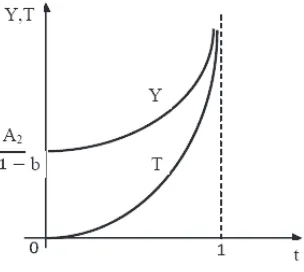
1. For given autonomous spending (all else being equal), equilibrium output is a decreasing function of t. At the same time, if we assume that t can take extreme values from 0 to 1, then the equilibrium output is maximum when t = 0 and minimum when t = 1. In particular,
2. For given autonomous spending, the net budget revenues (net taxes T) corresponding to equilibrium output are an increasing function of t. T is maximum when t = 1 and minimum when t = 0. In this case,
Tmax = A1 and Tmin = 0.
3. For given t, the equilibrium output and corresponding budget revenues increase (or decrease) when there is an increase (or decrease) in autonomous spending A1, of which one of the elements is government purchases G0.
The curves in Figure 1 show that, all else being equal, in the standard Keynes-ian model, with a change in the average tax rate t the values of equilibrium output and the corresponding net budget revenues change. Here we should point out that a change, an increase, for example, in A1 causes simultaneous upward movement of the curves corresponding to T and Y.
With aggregate supply that does not depend on t, which takes place in model (1)–(6),8 the relationship between the average tax rate, equilibrium output, and budget revenues shown in Figure 1 can be considered true only when govern-ment purchases G0 and net taxes T do not depend on each other. Naturally, in such conditions, when the average tax rate rises and G0 is fixed, there is an outflow of some funds from economic circulation, which, all else being equal, has a negative effect on the amount of aggregate demand and causes a contraction of equilibrium output, as is shown in Figure 1.
However, in reality, T and G are quantities that depend on each other. In prac-tice, the value of G is generally planned, for the most part, depending on what the expected net tax revenues T are. Furthermore, the need for changes in the average tax rate t is determined precisely by the steady growth of government purchases.9 Hence, in the model of aggregate demand, G and T should be considered not as isolated from each other—as in (1)–(6)—but as related to each other.
Version II of the Keynesian model of aggregate demand
We now consider the connection between government purchases (G) and net taxes (T) using an equation for the government’s budget:
D = G + rB–1 – T = (G – T) + rB–1 (10)
In the case of a deficit budget, tax revenues are not enough to cover spending. Therefore, the government is forced to borrow an appropriate amount from the private sector, international financial organizations, other countries, or the central bank. Borrowing from the private sector is particularly common. This process is carried out directly by the state treasury, whose securities are sold to individuals, firms, commercial banks, and other financial institutions. The money obtained in this way at the expense of the state treasury is used, just the way tax revenues are, to cover government spending. Financing a deficit with credit from the private sector (debt financing) is the basic form of deficit financing and is widely used in most countries in the current conditions. However, there are individual exceptions, especially in developing countries, when the treasury borrows from the central bank to finance a deficit. In this case, the central bank actually purchases an appropri-ate part of the treasury’s debt and creappropri-ates “high-efficiency money.”11 As we know, such financing is called monetization of the deficit. Without dwelling here on the positive and negative points of financing a budget deficit in these ways, we only point out that a budget cannot be constantly in deficit. There are periods when it is in surplus. In such cases, the government uses the surplus to repay or reduce the accumulated debt, or to create a reserve fund.
For simplicity, in what follows we use D to represent a deficit and B to represent government debt. At the same time, if necessary, we will specify the content of these quantities more precisely.
Equation (10) shows that the total budget deficit D is divided into two parts. One of them (G – T) is called a primary deficit when it is positive, and a positive primary balance when it is negative;12 and the other, rB
necessary to service it may be so high that the budget as a whole is in deficit, even in the case of a positive primary balance.
As we see, the amount of government debt at the beginning of the period de-termines how much the current budget is in deficit. For its part, the budget deficit is also a basis for the origin and growth of debt. Or rather, a budget deficit in the current period fosters the growth of government debt at the beginning of the next period. In general, the following relationship is valid:13
B = B–1 + D,
where B–1 and B are the values of government debt at the beginning and end of the period, respectively.
In this relationship we take into account the value of D from (10). Using simple operations, we get an equation that can be used to determine government debt based on the primary budget deficit as:
B = (G – T) + (1 + r)B–1. (11)
We will assume that B–1 in (11) is fixed and is a given quantity. This is a natural assumption, since the amount of B–1 is completely determined by decisions that the government has made in past periods. We will also assume that the value of the debt B at the end of the period is exogenously planned in the government bud-get and, if necessary, can be changed by taking on new debt or reducing current spending. As for government purchases G, they are tied to T and are determined from (11) as follows:
G = T + (B – (1 + r)B–1). (11a)
Consequently, we understand that the amount of government purchases is determined, on the one hand, by net tax revenues T and, on the other hand, by the policy that is conducted in relation to government debt. In other words, a change in G cannot be isolated—in the form in which it is traditionally considered in simple Keynesian models, including the model (1)–(6)—and it is always associated with a change in taxes or debt (or both at the same time).
We replace the condition G = G0 in model (1)–(6) with (11a), and we call the system modified in this way Version II of the Keynesian model. The equation for calculating equilibrium output will take the following form for this model:
Y = λ2A2, (12)
where
A2 = a + (B – (1 + r)B–1) + I0 + NX0, (13)
λ2
1
1 1
=
−b( − −t) t. (14)
spending A2, along with other elements, is not total government purchases G0, but only the part of them made at the expense of government debt incurred in the cur-rent period (B – (1 + r)B–1). According to (11), this quantity is determined by the primary budget deficit (G – T). Moreover, in Version II of the Keynesian model, the autonomous spending multiplier λ2 has a completely different form. While in conditions (7)–(9) the multiplier λ1 diminishes in relation to t, the opposite situ-ation takes place in this case, and the multiplier λ2 increases in relation to t. This circumstance leads to the following conclusions for Version II of the Keynesian model.
1. All else being equal, the creation or growth of government debt (creation or growth of a primary budget deficit (G – T)) has a positive effect on equilibrium output, while reduction of government debt or growth of government assets (creation or growth of a primary budget surplus (T – G)) has a negative effect. It is obvious that this situation is completely consistent with traditional Keynesian theory.
2. All else being equal, equilibrium output is an increasing function of the average tax rate t: dY/dt > 0. For given positive autonomous spending:
Ymin = A2/(1 – b), when t = 0; and Ymax = ∞, when t = 1.
This result, which is not the customary one for Keynesian theory, is interesting from the point of view that, according to Version II of the Keynesian model, in conditions of insufficient autonomous spending, one of the most important ways of increasing aggregate demand and boosting economic activity is to increase the average tax rate.
3. All else being equal, net budget revenues are an increasing function of t, and for given A2 > 0:
Tmin = 0, when t = 0; and Tmax = ∞, when t = 1.
Figure 2 shows curves representing the dependence of Y and T on the average tax rate in conditions of the model (12)–(14). Comparison of Figures 1 and 2 clearly indicates the difference between the results that follow from Versions I and II of the Keynesian model.
We dwell further on an interesting result that follows from the relationship (12)–(14). In characterizing the effectiveness of fiscal policy tools, researchers often turn to the theorem of the well-known economist Trygve Haavelmo.14 Based on a simple Keynesian model in which taxes are determined independently of Y, the theorem asserts that the balanced budget multiplier is equal to zero. In other words, according to this theorem, if the government increases its purchases and taxes by the same amount ∆G = ∆T, then output will rise by the same amount, that is, the equality ∆G = ∆T = ∆Y will be fulfilled. It can be shown that this theorem is also valid in Version II of the Keynesian model.15
of equilibrium, or, (G – T) = 0, which is the same thing. Then we can write:
G = T = tY,
where Y, according to conditions (12)–(14), is determined by the following equation:
Y A
Suppose that the government has decided to increase its purchases by increasing taxes. In the context of this model, doing so entails an increase in the average tax rate by some amount ∆t (∆t > 0, 0 < t + ∆t < 1). It is easy to see that such a change in t will cause a change in equilibrium output, and we get:
Y Y A
Since Y > 0 and ∆t > 0, from the derived expression it follows that the increase in output is positive.
We will show that ∆Y = ∆T = ∆G. To do this, we consider the pair of equations: T = tY, and
T + ∆T = (t + ∆t)(Y + ∆Y).
Subtracting the first equation from the second, we get: ∆T = t∆Y + ∆tY + ∆t∆Y.
According to (15), ∆tY on the right side of this expression is determined as ∆tY = (1 – t – ∆t) ∆Y. Taking this into account, we get ∆T = ∆Y. For its part, from (11a) it follows that ∆T = ∆G. Consequently, according to Version II of the Keynesian model, all else being equal, a tax increase fosters growth of output, but the overall effect obtained in this way is used only to provide for government purchases (the amount of household consumption remains unchanged, in spite of the growth of output; and investments and net exports are also unchanged, since, according to the assumption, these characteristics are given exogenously in the model and they are fixed). This result, together with equality (15), makes it possible to determine in advance how much the average tax rate should be raised in order to obtain the desired increase in government purchases ∆G without unbalancing the budget (or exceeding the planned deficit). In particular, since, all else being equal, with a tax increase, the equality ∆G = ∆Y will take place, from (15) it follows that the ap-propriate value of the tax increase for a given ∆G will be:
∆ ∆
This equation shows that the value of ∆t needed to obtain a unit increase of G is variable and depends on the existing level of the average tax rate t and the existing output Y. All else being equal, the higher the average tax rate or the existing output is, the less ∆t can be to obtain a unit increase of G.
To clarify why equilibrium output is increasing in relation to the tax rate in Version II of the Keynesian model, we will first explain the principle of operation of the multiplier λ2. We will use the standard method and consider a situation in which the amount of autonomous spending A2 increases by one unit. This change will cause a multistage process in each stage of which the equilibrium output and the income corresponding to it will grow by a certain amount. In keeping with these stages, we will designate the value of the corresponding increases as ∆Y(1), ∆Y(2), ∆Y(3), and so on.
It is clear that for the first stage ∆Y(1) = 1. From this unit increase of income, (1 – t) will remain in the private sector, and the other part (t) will go to the govern-ment’s budget in the form of taxes.
a unit of income additionally created in the economy. Therefore, [b(1 – t) + t ] rep-resents the joint marginal propensity of households and the government to purchase products and services.
Considering this circumstance, it is easy to see that for the third stage: ∆Y(3) = [b(1 – t) + t] ∆Y(2) = [b(1 – t) + t]2.
The increments of equilibrium output corresponding to subsequent stages are obtained analogously. Therefore, we will finally write:
∆Y = ∆Y(1) + ∆Y(2) + ∆Y(3) + ... = 1 + [b(1 – t) + t] + [b(1 – t) + t]2 + .... In a normal situation, 0 < b < 1 and 0 < t < 1. On the strength of this,
0 < [b(1 – t) + t] = [b + (1 – b)t] < [b + (1 – b)] = 1.
Consequently, the derived series is an infinitely decreasing geometric progres-sion, and the following equality is valid:
∆Y = [1 – b(1 – t) – t]–1 = λ2.
As we see, the main role in the multiplier process of creating equilibrium output is played by the joint marginal propensity of households and the government to purchase goods and services [b(1 – t) + t]. This parameter is the weighted value of two types of marginal propensity. One of them—b—is the marginal propensity of households to consume, and the other is the marginal propensity of the government to purchase products and services. In the model under consideration, the latter is equal to one, since, according to (11a), each additional unit of net tax revenue is fully spent on government purchases. The two values of marginal propensity (b and 1) are weighted according to 1 – t and t. Since the marginal propensity for government purchases of products and services is greater than b (0 < b < 1), the greater the value of t, the higher the joint marginal propensity [b(1 – t) + t] will be. And this means that, in the case of a high average tax rate, a large part of the income goes into the market in the form of spending and, all else being equal, the level of equilibrium output is also high.
From what has been said, it follows that when the marginal propensity of house-holds to consume is low in a country, and government purchases are planned in accordance with (11a), then to stimulate aggregate demand and increase equilibrium output, it is advisable to raise the average tax rate. At the same time, it should be taken into account that implementing this measure will not affect the total amount of household consumption and will only increase the part of output that will go to providing for government purchases.16
Version III of the Keynesian model of aggregate demand
suppose that only a certain part of the net taxes going to the budget is used for purchases, and the rest is used to service government debt and create a reserve fund. In addition, we will assume that part of the government purchases is determined exogenously and does not depend on taxes. In such conditions, the correlation between G and T can be expressed by the following linear function:
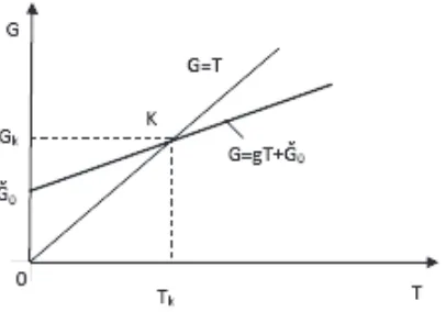
G = gT + G}0, (17)
where G}0 is the autonomous value of government purchases the amount of which does not depend on taxes and is determined exogenously. In conditions of insufficient tax revenues, this part of purchases can be made through borrowing; and g is the marginal propensity for government purchases. This parameter should be seen as exogenously regulated. Based on the situation existing in the economy, the government can increase or decrease the value of g, but in any case the marginal propensity to purchase must satisfy the condition 0 ≤ g ≤ 1, which is a fairly natural requirement.
Figure 3 shows that in the case of (17), if the amount of net taxes going to the budget T is less than Tk, then (G – T) > 0. Consequently, there is a primary budget deficit. If T > T
k, then there is a primary budget surplus (positive primary balance). And finally, a
bal-anced primary budget is reached at the point K, at which time Gk = Tk = G}0/(1 – g). In model (1)–(6), we replace the condition G = G0 with (17) and call the system thus obtained Version III of the Keynesian model. It is easy to establish that, accord-ing to this version, equilibrium output is determined by the followaccord-ing equation:
Y = λ3A3, (18)
where:
A3 = a + I0 + G}0 + NX0, (19)
λ3
1
1 1
1 1
=
As we see, in this model it is not the total amount of government purchases G that participates in the creation of autonomous spending A3, along with the elements a, I0, and NX0, as is traditional in the Keynesian model of aggregate demand, but a part of this amount G}0: autonomous government purchases, that is, purchases whose amount does not depend on net taxes going to the budget. Consequently, the autonomous spending multiplier λ3 is also different. The latter is determined by the joint marginal propensity of households and government to purchase products and services [b(1 – t) + gt], which is the weighted average of b and g. Comparing (9), (14), and (20), we notice that the multipliers λ1 and λ2 are particular cases of λ3. specifically, λ1 is derived from λ3 in the case when g—the marginal propensity for government purchases—is equal to zero;17 and if g = 1 in (20), then λ3 turns into λ2.
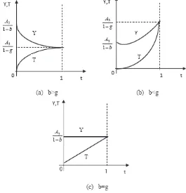
Previously, when considering Versions I and II of the Keynesian model, it was shown that changes in the average tax rate t affect equilibrium output differently in the cases when g = 0 and g = 1. Generalization of this fact gives us (18)–(20), from which it follows that in the Keynesian model the role of the average tax rate is determined by the relationship between the marginal propensity to consume b and the marginal propensity for government purchases g. When b > g, a rise in the average tax rate lowers the joint propensity of households and the government to purchase products and services [b(1 – t) + gt]. Therefore, all else being equal, an increase in t causes a reduction in equilibrium output. And in the opposite case (i.e., when b < g), an increase in the average tax rate causes growth of the joint marginal propensity of households and the government to purchase products and services, which, all else being equal, is a condition that fosters the growth of ag-gregate demand and, consequently, equilibrium output. And finally, when b = g, then both the joint marginal propensity of households and the government to purchase products and services and aggregate demand are indifferent to t.
Figure 4 shows curves corresponding to equilibrium output and net budget revenues determined in relation to t for Version III of the Keynesian model, with different possible combinations of the values of b and g.
From the analysis done using the versions of the Keynesian model examined above, we can draw the following conclusion. The effect of an increase (or decrease) in the average tax rate and taxes as a whole on aggregate demand is not unequivo-cally negative (or positive), as it is customarily presented in canonical form in contemporary macroeconomic textbooks.18 Depending on what the values of the marginal propensity to consume b and the marginal propensity to purchase g are, in the general case a tax increase can cause either a reduction or growth of aggregate demand. At the same time, since g is a parameter that the government can easily regulate, by selecting its appropriate value the government can purposefully use a tax increase to conduct a stimulating or inhibiting economic policy.
designate the expected changes as ∆Y, ∆T, ∆G, and ∆C.
It is easy to see that the change in equilibrium output is calculated in the fol-lowing form:
∆
∆ ∆
Y A
b t t g b
A
b t g b
A t g b
b t g
=
− − + − − − − − =
= −
− −
3 3
3
1 1
1
( ) ( )( ) ( ) ( )
( )
[( ) ( −−b)][(1− − +b) (t ∆t g)( −b)].
Considering the values of Y from system (18)–(20), this equation can finally be written as:
∆ ∆
∆
Y t g b Y
b t t g b
= −
− − + −
( )
[(1 ) ( )( )].
(21)
To determine ∆T, we transform (21) as follows:
∆t(g – b)Y = (1 – b)∆Y – t∆Y(g – b) – ∆t∆Y(g – b).
As a result of regrouping and combining similar terms, we get:
(∆tY + t∆Y + ∆t∆Y)(g – b) = (1 – b) ∆Y.
Since in the case of g ≠ b, ∆T = ∆tY + t∆Y + ∆t∆Y, while in the case of g = b, ∆T = ∆tY, the increase from net taxes has to be calculated according to the equation:
∆ ∆
According to (17), ∆G = g∆T. Consequently, the amount of increase in govern-ment purchases corresponds to the equation:
As for the increase in household consumption, based on function (2), it is cal-culated as follows:
We will analyze equations (21)–(24) and the conclusions stemming from them. First, we call attention to (21). It is easy to verify that in a normal situation the value of the denominator on the right side of this expression satisfies the condition [(1 – b) – (t + ∆t)(g – b)] > 0. Therefore, when t increases (i.e., when ∆t > 0, the
Consequently, only in certain cases does an increase in t cause growth of equilib-rium output.19 But then, from (22)–(24) it follows that the signs of ∆T, ∆G, and ∆C do not depend on the relationship of the parameters g and b. In general, disregard-ing some insignificant exceptions, with an increase in t net taxes and government purchases grow, and the amount of consumption decreases. More specifically, equations (22)–(24) indicate the following interesting circumstances.
Second, all else being equal, an increase in t does not change the amount of the budget deficit (or surplus) in only one case: when the marginal propensity to purchase g = 1. In this case, ∆T = ∆G. With any other value of the marginal pro-pensity to purchase, net taxes will rise more than government purchases if there is an increase in t, and this will create an opportunity to reduce the deficit (if there is one) or to create and increase a surplus:
∆ ∆
Third, it is easy to see that, all else being equal, in all cases of a change in t, the following equality is fulfilled:
∆G + ∆C = ∆Y, (28)
in which ∆G and ∆C have different signs. In particular, when t increases, then, regardless of whether ∆Y is positive or negative, ∆G ≥ 0 and ∆C ≤ 0. When the marginal propensity to purchase g = 1, the amount of consumption does not change (∆C = 0), and the entire growth of output goes to government purchases (∆G = ∆Y > 0). When g = 0, the situation is directly opposite. In this case, ∆G = 0, and a tax increase reduces consumption and output by the same amount (∆C = ∆Y < 0). From equations (28) and (25), it follows that, in the general case, with an increase in t, ∆G and ∆C are in the following relationship to each other:
Consequently, when g > b, with an increase in t, purchases will grow more than consumption is reduced. This circumstance determines the grow of aggregate spend-ing, as a result of which output Y also grows. And on the other hand, when g < b, consumption decreases more than purchases grow. In turn, this causes a decrease in aggregate spending and output.
Notes
1. For a survey of this concept, see, for example, V. Andrianov, “Gosudarstvo ili pynok? Keinsianstvo ili monetarism?” Obshchestvo i ekonomika, 2008, no. 10–11.
2. In contemporary economics, the role of fiscal policy and the tax system in not lim-ited to their effect on aggregate demand. A new doctrine emerged in the 1970s (supply-side economics), in which taxes and the tax system came to be seen as a purely fiscal tool that the government can use to stimulate business activity not through aggregate demand, but through reduction of the tax burden. However, this aspect of taxes is not addressed in this article. For more details about the role of taxes and tax policy in government regulation of the economy, see, for example, E.B. [A.B.] Atkinson and Dzh.E. Stiglits [J.E. Stiglitz],
Econom-ics] (Moscow: Aspekt Press, 1995); Dzh.E. Stiglits, Ekonomika gosudarstvennogo sektora
[Economics of the Public Sector] (Moscow: MGU INFRA-M, 1997); L.I. Iakobson, Gosu-darstvennyi sektor ekonomiki (Moscow: GU VShE, 2000).
3. See, for example, R. Dornbush [Dornbusch] and S. Fisher [Fischer], Makroekonomika
[Macroeconomics] (Moscow: MGU INFRA-M, 1997), pp. 93–97; N.G. Menk’iu [Mankiw],
Makroekonomika [Macroeconomics] (Moscow: MGU, 1994), pp. 374–84; Dzh. Saks [J. Sachs] and F.B. Larren [Larrain], Makroekonomika. Global’nyi podkhod [Macroeconomics in the Global Economy] (Moscow: Delo, 1996), pp. 405–12; O. Blanchard, Macroeconomics (Upper Saddle River, NJ: Prentice Hall, Pearson Education International, 2005), pp. 116–18.
4. Iu. Ananiashvili, “Vliianie nalogov na sovokupnyi spros,” Ekonomika da biznesi,
2008, no. 3 (in Georgian).
5. See, for example, Dornbush and Fisher, Makroekonomika, pp. 72–112; Mankiw,
Makroekonomika, pp. 366–84.
6. A lump-sum, or fixed, tax is one whose amount does not depend on the tax base. 7. The concepts of progressive and regressive taxation are defined in various ways in the economic literature (see, e.g., V.S. Zanadvorov, “Teoriia nalogooblozheniia,” Ekonomicheskii zhurnal VShE, 2003, no. 4). The approach used in our case is the one that Atkinson and Stiglitz rely on (Atkinson and Stiglits, Lektsii po ekonomicheskoi teorii gosudarstvennogo sektora,
p. 50). Taxation is progressive when the average tax rate rises with income growth. In the case of regressive taxation, the average tax rate decreases with an increase in income.
8. The assumption, all else being equal, is used to clearly establish the direction of the average tax rate’s influence on aggregate demand. Meanwhile, there is extensive literature studying the effect of the tax burden and the average tax rate on the level of business activity of individual economic agents and on the amount of aggregate output (supply) as a whole. See, for example, A. Bobrova, “O kriterii optimal’nogo nalogovogo bremeni,”
Obshchestvo i ekonomiki, 2005, no. 10–11; N. Kochetov, “Ob otsenke nalogovoi nagruzki na finansovye potoki predpriiatii,” Obshchestvo i ekonomika, 2006, no. 9; E.V. Balatskii [Balatsky], “Analiz vliianiia nalogovoi nagruzki na ekonomicheskii rost s pomosch’iu proizvodstvenno-institutsional’nykh funktsii,” Problemy prognozirovaniia, 2003, no. 2; Iu. Ananiashvili and V. Papava, Nalogi, spros i predlozhenie: laffero-keinsianskii podkhod
(Tbilisi: Siakhle, 2009) (in Georgian).
9. According to Wagner’s law, demand for public goods rises faster than demand for private goods, which is gradually saturated. Therefore, consumers are willing to give up more and more of their income as taxes funding the production of public goods (M.G. Kolosnit-sina, “Ekonomika obshchestvennogo sektora: gosudarstvennye raskhody,” Ekonomicheskii zhurnal VShE, 2003, no. 3, p. 390).
10. Public debt includes the loans taken internally in the private sector (domestic debt) and outside the country in various financial institutions and states (foreign debt).
11. Saks and Larren, Makroekonomika. Global’nyi podkhod, p. 290. 12. Dornbush and Fisher, Makroekonomika, p. 587.
13. See, for example, Blanchard, Macroeconomics, p. 579.
14. See, for example, L.S. Tarasevich, V.M. Gal’perin, P.I. Grebennikov, and A.I. Leusskii,
Makroekonomika (Izdatel’stvo SPbGUEF, 1999), p. 78.
15. It is not possible to prove the validity of this theorem based on Version I of the Keynesian model, or model (1)–(6), since government purchases and taxes are not a priori interrelated in it.
17. Zero marginal propensity to purchase does not mean that no purchases are made. The point is that the concept of marginal propensity to purchase is understood as spending on the acquisition of goods and services that the government takes upon itself from an additional unit of net taxes. Since the government can make purchases through borrowing or from nontax revenues, with a zero value of g it is entirely possible that G is positive. In model (1)–(6), as well as in the simple modification of it that is widely used in macroeconomic textbooks to illustrate the results of fiscal policy, it is actually implicitly understood that government purchases are made precisely through borrowing or from nontax revenues.
18. See, for example, Dornbush and Fisher, Makroekonomika, pp. 93–97; Mankiw,
Makroekonomika, pp. 374–84; Saks and Larren, Makroekonomika. Global’nyi podkhod,
pp. 405–12; Blanchard, Macroeconomics, pp. 116–18.