RETRIEVING FOREST STRUCTURE VARIABLES FROM VERY HIGH RESOLUTION
SATELLITE IMAGES USING AN AUTOMATIC METHOD
B.Beguet1,2, N.Chehata1,3, S. Boukir1and D. Guyon2
1EA 4592 G&E Laboratory, University of Bordeaux, 1 All´ee F.Daguin, 33607 Pessac Cedex, France 2INRA, UR1263 EPHYSE, 33140 Villenave d’Ornon, France
3LISAH UMR 144, IRD, El Menzah 4, Tunis, Tunisia 1[email protected],2[email protected]
Commission VII/1
KEY WORDS: Forestry, Modelling, Texture, Multi-resolution, Quickbird
ABSTRACT:
The main goal of this study is to define a method to describe the forest structure of maritime pine stands from Very High Resolution satellite imagery. The emphasis is placed on the automatisation of the process to identify the most relevant image features, exploiting both spectral and spatial information. Our approach is based on linear regressions between the forest structure variables to be estimated and various spectral and Haralick’s texture features (derived from Grey Level Co-occurrence Matrix). The main drawback of this well-known texture representation is the underlying parameters (window size, displacement length, orientation and quantification level) which are extremely difficult to set due to the spatial complexity of forest structure. To tackle this major issue, probably the main cause of poor texture analysis in practice, we propose an automatic feature selection process whose originality lies on the use of image test frames of adequate forest samples whose forest structure variables were measured at ground. This method, inspired by camera calibration protocols, selects the best image features via statistical modelling, exploring a wide range of parameter values. Hence, just a few samples are required to build up the test frames but allow a fast assessment of thousands of descriptors, given the large number of tested combinations of parameters values. This method was developed and tested on Quickbird panchromatic and multispectral images. It has been successfully applied to the modelling of 7 typical forest structure variables (age, tree height, crown diameter, diameter at breast height, basal area, density and tree spacing). The coefficient of correlation,R2, of the best single models for 6 of the forest variables of interest, estimated from the test frames, ranges from 0.89 to 0.97. Only the basal area was weakly correlated to the considered image features (0.64). To improve the results, combinations of panchromatic and or multi-spectral features were tested using multiple linear regressions. As collinearity is a very perturbing problem in multi-linear regression, this issue is carefully addressed. Different variables subset selection methods are tested. A new stepwise method, derived from LARS (Least Angular Regression), turned out the most convincing, significantly improving the quality of estimation for all the forest structure variables (R2 >0.98). Validation is done through stand ages retrieval along the whole site. The best estimation results are obtained from subsets combining multi-spectral and panchromatic features, with various values of window size, highlighting the potential of a multi-scale approach for retrieving forest structure variables from VHR satellite images.
1 INTRODUCTION
Many studies have focused on estimating forest parameters from remote sensing data since the early years of satellite imagery. The accuracy in retrieving forest stand variables such as stem volume, tree height and basal area from different image sources depends on their spatial resolution (Hyyppa et al., 2000). While SPOT or Landsat TM data give low correlation performance, aerial pho-tographs provide highly significant information. Using SPOT im-ages, (Wunderle et al., 2007, Wolter et al., 2009, Castillo et al., 2010) retrieve some forest stand attributes, exploiting image tex-ture, with a good accuracy. Over the last decade, a growing num-ber of Very High Resolution (VHR) remote sensing data from various spatial sensors has become available. The spatial reso-lution of the provided images is comparable to the one of aerial photographs. Some recent studies (Kayitakire et al., 2006, Feng et al., 2010, Proisy et al., 2007, Ozdemir and Karnieli, 2011, Song et al., 2010) have shown the potential of VHR imagery for forest inventory applications thanks to the strong relationship between forest spatial structure and image texture at stand level. In this paper, we aim to fully exploit the potential of texture features, extracted from VHR satellite images, in describing typical forest variables, with a particular emphasis on automatic parameter tun-ing, one of the major issues in texture analysis.
VHR imagery provides a meaningful textural information.
struc-ture. To tackle this major issue, probably the main cause of poor texture analysis in practice, an automatic feature selection pro-cess that explores a wide range of texture parameter values is a worthwhile solution to investigate.
The objective of the present study is to provide a fully automatic method to retrieve the most correlated texture features with the following forest structure variables: crown diameter, density and tree spacing which induce less or more texture in the image de-pending on the image spatial resolution. Complementary forest structure variables are also considered as tree height, diameter at breast height and basal area, as well as stand age which can be considered as a synthetic forest variable. The height of top of tree also contributes to image texture, in particular since it impacts on the length of its shadows according to the solar elevation or to the view zenith angle of the sensor. Texture analysis is based on GCLM with an automatic selection process of the features and their parameterization.
To achieve optimal results, some combinations of panchromatic and/or multi-spectral features were tested using multiple linear regressions between ground measured variables and image fea-tures. As collinearity is a very perturbing problem in multi-linear regression, this issue is carefully addressed through a new vari-able subset selection algorithm that has never been involved in re-mote sensing forestry : LARS (Least Angular Regression) (Efron et al., 2004), and outperformed other existing variable subset se-lection techniques. The developed method was assessed on mar-itime pine stands covering a large forest structure diversity from Quickbird images.
2 MATERIAL
2.1 Study site
The Nezer site is located in a large forest of maritime pine (Pinus pinaster Ait.) in southwestern France. Its surface is nearly flat. It is composed of maritime pine even-aged stands which are in-tensively managed. Their size is variable from approximately 4 to 50 ha. They are often circled by firebreak clearings or roads. The pine trees are planted in rows 4 m apart, which are oriented West-East in most of stands.
2.2 Field data
Measurements of forest structural variables were made on 12 stands at the end of year 2003. The trees sampled in each stand were located within a 80m×80m square plot representative of the forest structure in the 200m×200m area that encloses it. Crown
diameter (Cd), stand density (Nah), tree Height (Ht), Diameter at breast height (Dbh), and Basal area (Ba) were measured. Tree Spacing (Sp) is estimated as an empirical function of density, this allows a linearization of density variations.
Sp(m) =
√ 20000
√
3density(tree/ha) (1)
Age of the sampled stands is ranged from 13 to 51 years. The variation range of the forest variables are presented in Table 1. As expected, due to allometric constraints, a strong correlation is observed between age, Cd, Dbh, Ht, Nah and Sp. Only Ba, which strongly depends on the changes in density and Dbh due to thinning, is not as correlated to other structural variables. The exact age is known for all stands of the site from forest manager’s archives. Only 184 stands, with available remote sensing data, are involved in this study.
2.3 Remote sensing data
Quickbird is among the satellite sensors with the highest spatial resolution and its spectral characteristics are suitable for forest
Cd (m) Nah (tree/ha) Sp (m) Ht (m) Dbh (m) Ba (m2/ha) Age (year) Min 2.9 189 3.0 9.2 0.15 20.2 13 Max 7.8 1253 7.8 24.6 0.46 33.2 51
Table 1:Range of variations of forest variables over 12 sampled stands
applications. This sensor has a spatial resolution ranging from 0.61 to 0.70 m in the panchromatic channel (Pan) and from 2.44 to 2.88 in the multi-spectral channels (MS), depending on the view angle, and a radiometric resolution of 11 bits. The image, acquired on the 6th of October 2003, was delivered as a sensor corrected standard product of an excellent quality, with no clouds and a view angle of 19◦. All channels (MS and Pan) were well
co-registered (registration error<1 pixel). As the image was acquired in October, a period where under-tree green biomass amount is rather low, the spatial variations in understory vege-tation reflectance were probably low.
3 METHODS
3.1 Features
We considered first order texture features (mean and variance) and second order GLCM texture features to describe the spatial relationship between a pixel and its neighborhood. (Haralick et al., 1973) defined 14 texture features derived from GLCM. Some of them are considered as particularly relevant for image analysis on forest applications (Franklin et al., 2001, Coburn and Roberts, 2004, Kayitakire et al., 2006, Murray et al., 2010, Wunderle et al., 2007, Ozdemir and Karnieli, 2011, Castillo et al., 2010). These studies generally involved one spatial resolution, either panchro-matic or multi-spectral. To our knowledge, only Wolter (Wolter et al., 2009) has combined features at both resolutions, but from var-iogramm and not GLCM as in the present work. All texture mea-sures were calculated on both Panchromatic and Multi-spectral bands. We used the four available spectral bands (Blue (B), Green (G), Red (R), Near Infra Red (NIR)) and the well-known NDVI (Normalized Difference Vegetation Index). We considered the eight most used Haralick’s features in remote sensing forestry (Wunderle et al., 2007, Ozdemir and Karnieli, 2011, Castillo et al., 2010) :
Haralick’s Correlation (harcorr)= f8 = ∑
i,j(i,j)g(i,j)−µ
2
t
σ2t where
µtandσtare the mean and standard deviation respectively of the row (or
column, due to symmetry) sums. Above,µ=∑
i,ji·g(i, j) =
Besides, we added another feature, pantex, which represents the min value of the contrast in 8 directions (Pesari et al., 2008). This provides an anisotropic feature. GLCM parameters are: radius of the moving windowr (window size = 2 r+1), displacement
considered, setting nbbin=8, as traditionally used in literature, ap-pears to be sufficient. As there is no way of knowinga priorithe
Data r(pixel) d(pixel) o(degree) Pan 5-25 step: 5 1-10 step :1 0-135 step: 45 MS 3-12 step: 3 1-4 step:1 0-135 step: 45
Table 2:GLCM parameter range values
appropriate GLCM parameters to use for our data, we chose to explore a wide range of parameter values. The first order features were calculated using the same window radius values.
3.2 Automatic feature selection
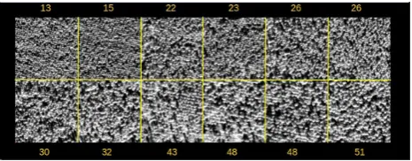
Test frame : We propose an automatic feature selection pro-cess whose originality lies on the use of test frames of adequate forest samples where the structure variables were measured from ground. This method, inspired by camera calibration protocols, selects the best image features via statistical modelling, exploring a wide range of parameter values. Hence, just a few samples are required to build up the test frames but allow a fast assessment of thousands of descriptors, given the large number of tested com-binations of parameters values. Compared to more traditional su-pervised methods, which are very costly in terms of field surveys and time-consuming, our method requires a slight supervision. Furthermore, in the context of texture analysis, which involves high computational costs, the use of test frames appears as an ap-pealing way to explore a wide range of texture parameters which would be impractical in case of large image samples. The for-est tfor-est frame is constructed with 12 small image samples corre-sponding to the field measurements (cf. Figure 1). Square plot areas are centered on the field measurement area, with a width of 200 pixels for Pan and 50 pixels for MS (around 120 meters on the ground). Maximum and minimum values of the whole test frame are used to construct the GLCM’s quantification levels (this guarantees that onlyforestpixels will be used). For each square plot, the average (M) and the variance (V) of all features were saved for statistical analysis.
Two approaches were tested for statistical modelling; linear re-gression where a forest variable is described by a single texture feature and thus exploiting only one spatial resolution. The sec-ond approach is a multi-scale method based on multiple regres-sions using several Pan and MS features to estimate a given forest variable.
Figure 1:Panchromatic test frame, sorted by increasing age
Single variable linear regressions : To retrieve forest struc-ture variables from VHR imagery, we relied on linear regressions between each of the 7 typical forest structure variables to be esti-mated and various textural features (first order and Haralick’s fea-tures). The Pearson correlation coefficientR2is used to analyze the correlation between each forest variable and texture features. Each forest variable is modeled as a function of a single texture feature. The best model for each variable is obtained automati-cally by selecting the one with the highestR2.
Towards a multi-scale approach : The novelty in this approach is to combine features at different spatial and spectral resolutions using Pan and MS bands, and requiring different parametriza-tions, in an automated way. To achieve this goal, multiple re-gressions are used. Considering a large number of features, that are likely correlated, the challenge is in minimizing the multi-collinearity on subset solutions in order to generate stable models and avoid overfitting. This can be done using the Variance In-flation Factor (VIF), a good multicollinearity detector which is defined as follows for any variable j involved in multiple regres-sion :
vj= 1 1
−R2j whereR
2
jis the correlation coefficient from a
regres-sion of predictorjagainst the remaining predictors. The higher
vj(VIF), the higher the collinearity between the predictorjand
the remaining predictors is high. VIF equals to 1 if there is no correlation between features. A critical value of 4 is usually used (Castillo et al., 2010).
Different subset selection methods exist for multiple regressions. In this study, we compared the performances of three methods : the classic step-by-step forward method, a LASSO (Least Ab-solute Shrinkage and Selection Operator) method, and a forward stepwise approach based on LARS (Least Angular Regression) (Efron et al., 2004). The LARS algorithm is a novel forward step-wise method. Unlike the classic Forward method which adds the variable leading to the highest F-statistic, the LARS algorithm adds the variable that better explains the current residuals. The LASSO minimizes the usual sum of squared errors, with a bound on the sum of the absolute values of the coefficients. LASSO and LARS stepwise have the same computational costs as ordinary least square regression. To compare the models performances, the PRESS (Predicted Residual Error Square Sum) (Allen, 1974) is used. This criterion is defined as :
P RESS=∑n
i=1(yi−yˆi(−i))
2whereyˆ
i(−i)is the prediction
for observationiwhen this observation is used as a supplementary data for the corresponding regression. This criteria is equivalent to a leave-one-out cross validation : the prediction error for an observation is obtained with a model constructed without this ob-servation.
In addition, the Mallow’sCpstatistic is used to decide the appro-priate number of variables to keep in the model. This statistic’s expression is given by:
Cp= (SSEp
SSE2)−(n−2p)whereSSE2is the mean square error
of the full model, andSSEpis the residuals square sum of the
model containing thepvariables of interest. The stop condition is whenCp=p, wherepis the number of variables (Efron et al., 2004).
The subset selection method that minimizes the VIF will be pre-ferred. We aim to fully automatically find a good subset solution without any manual intervention.
4 RESULTS AND DISCUSSION
All image features extractions are based on the use of the Or-feoToolbox library (OTB1) (Inglada and Christophe, 2009), sta-tistical analysis is based on Rproject. The whole is managed us-ing Python programmus-ing language.
4.1 Single solutions
The tested dataset is made up of 2894 and 4760 feature descrip-tors for Pan and Ms respectively. For each forest variable, numer-ous significant linear relationships with image features are found
(considering a p-value<0.01 forR2). No anomaly was observed on the normal hypothesis for those features. Features with the highest absolute correlation coefficient are presented in Table 3 for Pan and MS bands separately. All model parameters estima-tions are significant considering a 1% level.
Variable Band Feature r d 0 moment R2 pvalue RMSE Cd Pan inertia 10 6 45 M 0.943 1.515e-07 0.342
PIR inertia 3 2 90 M 0.940 1.924e-07 0.350 Nah Pan inertia 25 1 90 M 0.943 1.459e-07 75.282
B corr 6 3 0 V 0.970 5.350e-09 54.153 Sp Pan inertia 25 1 45 M 0.928 4.881e-07 0.388
PIR invdif 6 3 0 M 0.926 5.390e-07 0.392 Ht Pan inertia 25 1 45 M 0.897 2.901e-06 1.428 PIR invdif 6 3 0 M 0.923 6.636e-07 1.233 Dbh Pan inertia 25 6 45 M 0.905 1.911e-06 0.027 PIR invdif 12 3 90 M 0.930 4.257e-07 0.023 Ba Pan inertia 25 7 45 V 0.610 0.002 2.567 NDVI corr 3 1 0 M 0.641 0.001 2.463 Age Pan invdif 25 6 45 M 0.893 3.564e-06 4.106 G variance 12 M 0.848 2.095e-05 4.892
Table 3:Forest structure variables and their best image descriptors
The best descriptors were found for density and crown diame-ter (which have the biggest impact on image texture) which are the Blue band correlation and the Pan inertia respectively. All other forest variables are well described except for the basal area. This result was expected considering literature (Kayitakire et al., 2006). Performances are similar for Pan and MS on this reduced set of stands. In addition, second order texture features (GLCM) clearly appear to be the most descriptive of forest structure, only one first order texture (green band variance) has been selected for age estimation. Inertia and inverse difference are the most fre-quently selected GLCM texture features in this study. The near infra red is the most relevant band for MS. A window radius of 25 is the best for Pan, it varies between 3 and 12 for MS. The optimal displacement for Pan is either 6 or 1 pixel with a 45◦orientation
while for MS, the optimal displacement is of 3 pixels with a 0◦
or 90◦orientation.
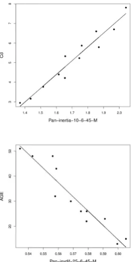
Figure 2: Relationship between forest structure variables and selected image features
Figure 2 shows some of the best achieved relationships between forest variables and image features. Linear presumptions are con-firmed and no alarming behaviors are noticeable on residual plots.
The variability of feature parameters shows that a wide range of parameters has to be tested to optimize the prediction preci-sion for a considered forest variable. Overall results are good compared to other works on VHR imagery. For instance, (Kay-itakire et al., 2006) found the following correlation coefficients with other texture features (correlation and contrast) from the panchromatic Ikonos band (1m) and 30 observations of spruce stands: 0.81, 0.76, 0.82, 0.82 and 0.35 for age, Ht , Dbh, density and Ba. RMSE reached 2, 0.4 and 7 for Ht, Dbh and Ba. One has to be cautious though not to draw fast conclusions from these results due to the limited data (12 observations) that has been used in the estimation process.
4.2 Multiple solutions
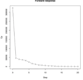
The determination of the best subset selection method was car-ried out by testing the three methods (classic Forward, Lasso and LARS stepwise) on all variables with both Pan and Ms datasets. Results are shown only for the estimation of age for which the highest number of observations is available (184 versus 12 for the other variables). The three methods behave similarly for all tested forest variables. The number of variables was fixed to three according the Cp statistic. Figure 3 shows the Cp’s curve (which indicates the gain when adding a variable at each step) for the LARS stepwise selections. The subset selection methods for
re-Figure 3:Cp’s curve for LARS stepwise selection on panchromatic data
trieving the age variable are compared in Table 4 and Table 5 using Pan and MS data respectively. For each model, we show the LMG (initials of the authors who first proposed the method) statistic to estimate the contribution of each variable on the ob-tained model (Gromping, 2006). LMG averages the sum of se-quential squares for all possible arrangements of the variables in the model. One can observe that the LARS stepwise selec-tion generates a subset without multicollinearity (VIF close to 1). The forward selection leads to the best prediction performance considering the PRESS criteria, however VIF values are criti-cal (>4). The lasso selection proposes a more balanced model (considering the contribution of variables (LMG)) but the solu-tion suffers from multicollinearity too.
Methods Band Feature r d 0 moment LMG VIF PRESS Forward Pan invdif 25 6 45 M 0.521 4.534 38.113
Pan clushade 25 5 90 M 0.393 2.779 Pan energy 10 3 0 M 0.084 2.247 Lasso Pan invdif 25 6 45 M 0.356 4.653 105.213
Pan inertia 20 8 0 V 0.320 6.247 Pan clushade 20 6 90 M 0.322 3.725 Stepwise Pan invdif 25 6 45 M 0.906 1.041 80.423
Pan inertia 25 3 45 M 0.078 1.069 Pan corr 25 2 0 V 0.015 1.102
Table 4:Comparison of subset selection methods in retrieving ages from panchromatic data (n= 12)
Methods Band Feature r d 0 moment LMG VIF PRESS Forward G variance 12 M 0.434 7.738 116.77
G clushade 3 1 0 V 0.393 5.299 PIR clushade 6 2 90 M 0.351 3.794 Lasso G variance 12 M 0.336 5.365 361.283
NDVI clushade 3 2 45 V 0.332 5.612 R corr 6 2 0 V 0.330 5.082 Stepwise G variance 12 M 0.819 1.118 115.731
PIR corr 6 2 45 M 0.038 1.039 R corr 9 4 0 V 0.142 1.081
Table 5:Comparison of subset selection methods in retrieving ages from multispectral data (n= 12)
quality of predictions in all cases including the basal area com-pared to single regressions (Table 3). One can observe that most
Band Feature r d 0 moment LMG VIF PRESS RMSE Cd Pan inertia 10 6 45 M 0.906 1.018 0.219 0.09
G corr 9 3 90 V 0.053 1.139 NDVI harcorr 12 1 0 V 0.040 1.144
Nah B corr 6 3 0 V 0.862 1.728 2640.916 10.875 B corr 6 3 45 M 0.086 1.968
Pan corr 20 8 45 V 0.051 1.602
Sp Pan inertia 25 1 45 M 0.928 1.247 0.254 0.09 Pan corr 5 3 90 V 0.033 1.110
Pan corr 10 5 45 M 0.037 1.130
Ht PIR invdif 6 3 0 M 0.871 1.124 5.887 0.402 R corr 9 4 0 V 0.114 1.061
PIR corr 3 2 45 M 0.014 1.073
Dbh PIR invdif 12 3 90 M 0.830 1.111 0.001 0.005 B corr 3 2 0 V 0.157 1.110
Pan inertia 15 1 45 V 0.011 1.003
Ba NDVI corr 3 1 0 M 0.786 1.134 10.859 0.487 Pan inertia 25 2 0 V 0.203 1.371
NDVI clushade 12 3 0 M 0.009 1.234
Age Pan invdif 25 6 45 M 0.841 1.046 84.538 1.287 Pan inertia 25 3 45 M 0.079 1.011
G corr 12 3 90 V 0.079 1.056
Table 6: Multiple solutions combining panchromatic and multispectral data (n= 12)
of the optimal subsets use jointly Pan and MS data which con-firms the relevance of a multi-scale approach. Besides, models are composed of features with various parameterizations. The VIF exhibits again a very low multicollinearity (close to 1) be-tween all the selected subsets of texture features, for every esti-mated forest variable. Hence, the subset selection method gen-erated a relevant solution, ensuring both high accuracy and low multicollinearity, in all tested cases. Compared to similar works on multi-linear regressions (Wolter et al., 2009), our approach tackles the multicollinearity problem in a more convincing way, being both a non parametric approach (no threshold to set) and completely automatic on both the selection of the subset of tex-ture featex-tures and the underlying optimal parameters (window size, displacement length and orientation). We chose to limit the range of Haralick parameters to experiment as a trade-off between accu-racy and efficiency, thus leading to a sub-optimal solution for all estimated forest variables. A broader range of descriptors could be easily considered to improve accuracy but at higher computa-tional costs.
4.3 Validation on stand age
All features were calculated following the same protocol for all the site stands as for the previous test frame. A square plot (120m) was defined around the center of each stand. The optimal sin-gle features for age prediction are presented in Table 7. Stand
Band Feature r d 0 moment R2 pvalue RMSE Pan invdif 10 8 45 V 0.706 <2.2e-16 5.665 G variance 3 M 0.663 <2.2e-16 6.068
Table 7:Best image features for age prediction (n= 184)
age varies from 4 to 51 years. The introduction of observations with more variability leads to linear relationships of lower signif-icance. Comparing these results with those obtained by 12 ob-servations, we can notice that the same best features are found for both Pan and MS data (Table 3). The obtained window ra-dius is lower, which could be explained by the presence of very young stands, corresponding to smaller texture structure. This shows that window size is very sensitive to tree size or tree spac-ing variations. The multi-scale approach combines features with
different parameters (especially window size and resolution, both strongly related to the intrinsic nature of the texture which could be more or less captured and retrieved depending on the set up of these important spatial parameters). It is a good way to capture a well adapted information. The LARS selection was then applied
Figure 4:Cp’s curve for age features selection
on the full dataset.The obtained variable subset is presented in Ta-ble 8 and the corresponding Cp’s curve in Figure 4. The optimal feature subset is not subject to multicollinearity, confirming the efficiency of the LARS subset selection. The predicted RMSE (obtained by leave-one-out validation) is 5.25 years, correspond-ing to 10% of the age dynamic over the site.
Band Feature r d 0 moment LMG VIF PRESS RMSE Pan invdif 10 8 45 V 0.510 2.551 3423.509 4.313 Pan harcorr 5 1 135 M 0.123 1.357
NDVI harcorr 12 4 0 M 0.067 1.697 Pan inertia 25 2 45 V 0.011 1.150 G corr 3 4 135 M 0.080 1.353 NDVI corr 9 2 135 M 0.054 1.798 Pan corr 5 2 45 V 0.043 1.276 PIR corr 9 1 45 M 0.134 1.276 R corr 6 3 45 M 0.017 1.042 NDVI corr 6 4 90 V 0.088 1.075
Table 8:Optimal image feature subset for age retrieval
Figure 5:Observed and predicted age on the whole site
The predicted variable is relevant for stands younger than 35 years old (Figure 5).
In pine maritime forest of southwestern France, the oldest stands (over 40 years) are often heterogeneous and their canopy cover is often open mainly due to the sylvicultural rules applied before the 70’s. Moreover, above a given age (about 35 years), the trees growth slows down and the forest variables tend to be plateauing with age. This explains why the correlation between observed and predicted age decreases for the oldest stands.
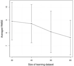
obtained an averaged RMSE ranging from 9 to 7.5 years. As we introduce a lot of randomness, the RMSE’s standard deviation is important. This highlights the strong influence of the choice of observations and their number on the relevance of the test frame construction.
Figure 6:RMSE variations of predicted age as a function of the obser-vation number (each point is the average of 100 experiments)
Finally, as crown diameter and spacing are strongly correlated with age we can expect for these forest variables a similar be-havior regarding the statistical analysis performances presented in this section.
5 CONCLUSIONS AND FUTURE WORK
This study provided an automatic method to retrieve forest struc-ture variables using spectral and Haralick’s texstruc-ture extracted from VHR optical satellite images. An automatic feature selection pro-cess whose originality lies on the use of image test frames of adequate forest samples was tested. This method allows a fast as-sessment of thousands of descriptors, exploring a wide range of parameter values. The best image features are selected via statis-tical modelling.
Seven typical forest structure variables were successfully mod-eled. Apart from the basal area, the regression coefficient,R2, of the best single models ranges from 0.89 to 0.97. Then, a multi-scale approach, combining panchromatic and/or multi-spectral features with different parameterizations, is proposed. The mul-ticollinearity problem is addressed carefully using the VIF crite-rion. Comparing three variable subset selection methods, a new stepwise method, derived from LARS, turned out the most con-vincing, significantly improving the quality of estimation for all the forest structure variables, including the basal area (R2 > 0.98). A validation on stand age retrieval over the whole site highlighted the potential of a multi-scale approach for retrieving forest structure variables from VHR satellite images. The whole protocol we have introduced can be easily applied to any other forest site data using site-specific test frames.
Our method will be applied on different sites, using other VHR sensors, expecting data from the new Pleiades satellite which has been successfully launched in December 2011.
ACKNOWLEDGEMENTS
This research was supported by the regional council of Bordeaux (R´egion Aquitaine) and CNES2 through the ORFEO program. The authors ac-knowledge INRA3for the VHR imagery and corresponding field data.
2Centre National d’Etudes Spatiales 3Institut National de Recherche Agronomique
REFERENCES
Allen, D. M., 1974. The relationship between variable selection and pre-diction. Technometrics 16:125, pp. 125–127.
Barbier, N., Couteron, P., Proisy, C., Malhi, Y. and Gastellu-Etchegorry, J. P., 2010. The variation of apparent crown size and canopy heterogeneity across lowland amazonian forests. Global Ecology and Biogeography 19, pp. 72–84.
Castillo, M. A., Ricker, M. and Jong, B. H. J. D., 2010. Estimation of tropical forest structure from spot-5 satellite images. International Journal of Remote Sensing 31-10, pp. 2767–2782.
Coburn, C. A. and Roberts, A. C. B., 2004. A multiscale texture analysis procedure for improved forest stand classification. International Journal of Remote Sensing 25, pp. 4287–4308.
Efron, B., Hastie, T. and Tibshirani, I. J. R., 2004. Least angle regression. The Annals of Statistics 32-2, pp. 407–499.
Feng, Y., Li, Z. and Tokola, T., 2010. Estimation of stand mean crown diameter from high-spatial-resolution imagery based on a geostatistical method. International Journal of Remote Sensing 31-2, pp. 363–378. Franklin, S. E., Maudie, A. J. and Lavigne, M. B., 2001. Using spatial co-occurence texture to increase forest structure and species composition classification accuracy. Photogrammetric Engineering & Remote Sensing 67-7, pp. 849–855.
Gromping, U., 2006. Relative importance for linear regression in r: The package relaimpo. Journal of Statistical Softaware 17, pp. 1–27.
Guyon, D. and Riom, J., 1996. Estimation de caract´eristiques foresti`eres `a partir d’images `a haute r´esolution spatiale (spot5). BUL. S.F.P.T. 141, pp. 46–50.
Haralick, R. M., Shanmugan, K. and Dinstein, I., 1973. Texture features for image classification. IEEE Transactions Systems, Man and Cybernet-ics pp. 610 – 621.
Huang, C., Song, K., Kim, S., Townshend, J. R. G., Davis, P., Masek, J. G. and Goward, S. N., 2008. Use of a dark object concept and support vector machines to automate forest cover change analysis. Remote Sensing of Environment 112(3), pp. 970–985.
Hyyppa, J., Hyypa, H., Inkinen, M., Engdahl, M., Linko, S. and Zhu, Y. H., 2000. Accuracy comparison of various remote sensing data sources in the retrieval of forest stands attributes. Forest Ecology and Manage-ment 128, 1-2, pp. 109–120.
Inglada, J. and Christophe, E., 2009. The orfeo toolbox remote sensing image processing software. In: IEEE International Geoscience and Re-mote Sensing Symposium.
Kayitakire, F., Hamel, C. and Defourny, P., 2006. Retrieving forest struc-ture variables based on image texstruc-ture analysis and ikonos-2 imagery. Re-mote Sensing of Environment 102, pp. 390–401.
M.Tuceryan, 1998. The Handbook of Pattern Recognition and Computer Vision (2nd Edition)(207-248). C. H. Chen, L. F. Pau, P. S. P. Wang. Murray, H., Lucieer, A. and R.Williams, 2010. Texture-based classifi-cation of sub-antarctic vegetation communities on heard island. Inter-national Journal of Applied Earth Observation and Geoinformation 12, pp. 138–149.
Ozdemir, I. and Karnieli, A., 2011. Predicting forest structural parameters using the image texture derived from worldview-2 multispectral imagery in a dryland forest, israel. International Journal of Applied Earth Obser-vation and Geoinformation 13, pp. 701–710.
Pesari, M., Gerhardinger, A. and Kayitakire, F., 2008. A robust built-up area precense index by anisotropic rotation-invariant textural measure. IEEE Journal of selected topics in applied earth observations and remote sensing.
Proisy, C., Couteron, P. and Fromard, F., 2007. Predicting and mapping mangrove biomass from canopy grain analysis using fourier-based textu-ral ordination of ikonos images. Remote Sensing of Environment 109, pp. 379–392.
Song, C., Dickinson, M. B., Su, L., Zhang, S. and Yaussey, D., 2010. Esti-mating average tree crown size using spatial information from ikonos and quickbird images: Across-sensor and across-site comparisons. Remote Sensing of Environment 114, pp. 1099–1107.
Wolter, T., Townsend, P. A. and Sturtevant, B. R., 2009. Estimation of forest structural parameters using 5 and 10 meter spot-5 satellite data. Remote Sensing of Environment 113, pp. 2019–2036.