Full Terms & Conditions of access and use can be found at
http://www.tandfonline.com/action/journalInformation?journalCode=ubes20
Download by: [Universitas Maritim Raja Ali Haji] Date: 11 January 2016, At: 22:14
Journal of Business & Economic Statistics
ISSN: 0735-0015 (Print) 1537-2707 (Online) Journal homepage: http://www.tandfonline.com/loi/ubes20
Modeling the Conditional Distribution of Daily
Stock Index Returns: An Alternative Bayesian
Semiparametric Model
Maria Kalli , Stephen G. Walker & Paul Damien
To cite this article: Maria Kalli , Stephen G. Walker & Paul Damien (2013) Modeling
the Conditional Distribution of Daily Stock Index Returns: An Alternative Bayesian Semiparametric Model, Journal of Business & Economic Statistics, 31:4, 371-383, DOI: 10.1080/07350015.2013.794142
To link to this article: http://dx.doi.org/10.1080/07350015.2013.794142
Accepted author version posted online: 06 May 2013.
Submit your article to this journal
Article views: 679
Modeling the Conditional Distribution of Daily
Stock Index Returns: An Alternative Bayesian
Semiparametric Model
Maria K
ALLIBusiness School, Canterbury Christ Church University, Canterbury, Kent CT2 7NF, UK ([email protected])
Stephen G. W
ALKERSchool of Mathematics, Statistics & Actuarial Science, University of Kent, Canterbury, Kent CT2 7NF, UK ([email protected])
Paul D
AMIENMcCombs Business School, University of Texas at Austin, Austin, TX 78712 ([email protected])
This article introduces a new family of Bayesian semiparametric models for the conditional distribution of daily stock index returns. The proposed models capture key stylized facts of such returns, namely, heavy tails, asymmetry, volatility clustering, and the “leverage effect.” A Bayesian nonparametric prior is used to generate random density functions that are unimodal and asymmetric. Volatility is modeled parametrically. The new model is applied to the daily returns of the S&P 500, FTSE 100, and EUROSTOXX 50 indices and is compared with GARCH, stochastic volatility, and other Bayesian semiparametric models.
KEY WORDS: Infinite uniform mixture; Markov chain Monte Carlo; Slice sampling; Stick-breaking processes.
1. INTRODUCTION
Financial managers as well as investors would like to be in a position to accurately forecast asset return movements. The underlying distribution of these returns affects their decisions. Their predictions on asset price movements will be inaccurate, leading to bad investment decisions, if the distributional assump-tions are not reflected in the financial data they are interested in.
The challenging task of modeling the conditional distribution of asset returns has been the subject of many studies. Some develop ARCH-GARCH-type models, first introduced in Engle (1982) and Bollerslev (1986), while others build on the stochas-tic volatility (SV) model first introduced by Taylor (1982). For a comprehensive list of models, see Taylor (2005), Tsay (2005), and Bollerslev (2008). The difficulty lies in developing a model that captures the complicated features of the returns’ distribu-tion, often referred to as stylized facts (see Cont2001; Poon and Granger2003). In this article, we build a GARCH-type model for the asset returns’ conditional distribution, which has a mode and a mean close to zero, and accounts for asymmetry, heavy tails, volatility clustering, and “leverage effects.”
The deterministic nature and ease of estimation of GARCH-type models makes them a popular choice. The basic setup of these models is
yt = htǫt fort =1,2, . . . , n, (1)
whereyt is the log return,ǫt is the innovation following some distributionFǫwith mean zero and varianceσǫ2 =1, andh
2
t is the volatility at timet,which is a function of previous volatil-ities and returns. The choice ofFǫ determines the conditional
distribution of returns and impacts on distributions of future returns.
The normal distribution had been a popular choice for Fǫ. However, it has been shown that GARCH-type models with normal innovations fail to capture the heavy tails and slight asymmetry of the conditional distribution of returns. Alterna-tive distributional choices include the Student’s-t distribution (Bollerslev 1987), the generalized error distribution (Nelson 1990), and a mixture of normal distributions (Bai, Russell, and Tiao 2003). Although these alternatives account for the heavy-tailed behavior of the distribution, they fail to cap-ture skewness. To account for both aforementioned feacap-tures, Gallant and Tauchen (1989) used Gram–Chalier expansions, while Hansen (1994) introduced the skewed Student’s-t dis-tribution, and Theodossiou (1998) considered the generalized
t-distribution. Recently, Chen, Gerlach, and Lu (2012) used the asummetric Laplace distribution. However, all these choices are constrained by the properties and parameters of the distribu-tional family to which they belong.
This article describes a Bayesian nonparametric approach to modeling the conditional distribution of returns by nonparamet-rically estimating Fǫ. Bayesian nonparametric models place a prior on an infinite-dimensional parameter space and adapt their complexity to the data. A more appropriate term is infinite-capacity models, emphasizing the crucial property that they allow their complexity (i.e., the number of parameters) to grow
© 2013American Statistical Association Journal of Business & Economic Statistics October 2013, Vol. 31, No. 4 DOI:10.1080/07350015.2013.794142
371
as more data are observed; in contrast, finite-capacity models assume a fixed complexity. For a book length review of Bayesian nonparametric methods, see Hjort et al. (2010).
The Dirichlet Process Mixture (DPM) model, an infinite mix-ture model, first introduced by Lo (1984) is the most popular Bayesian nonparametric model in financial econometric appli-cations (see Chib and Hamilton 2002; Hirano 2002; Jensen 2004; Griffin and Steel 2006; Leslie, Kohn, and Nott 2007; Shahbaba 2009; Jensen and Maheu 2010). The DPM model uses the Dirichlet process (DP; Ferguson1973) as a prior over the parameters of a normal distribution, with densityk(·), facil-itating the modeling of complex densitiesf(·).Under the DPM modelf(·) = k(·|θ)G(dθ),whereθ is the parameter vector andGis the unknown random distribution drawn from a DP.
In our approach to modeling the innovations’ distribution,
Fǫ, we depart from the DPM model in two ways. We use a stick-breaking prior (SBP) instead of a DP to generateG, and substitute the normal density with a scaled uniform density. The uniform density ensures unimodality and an asymmetry parameter allows us to capture the asymmetry in asset returns. Stick-breaking processes are more general than the DP, in fact the DP is a subclass. They can therefore adapt more flexibly to the data and together with the scaled uniform density can capture more accurately the heavy-tailed behavior. We believe that with this model we can better account for extreme events, which impact on the tail behavior of the returns’ distribution, by mitigating the risk of placing artificial modes at unusual points. We model the volatility dynamics using: the GARCH(1,1), the GJR-GARCH(1,1), and the EGARCH(1,1) models; the latter two can capture the “leverage effect.”
The structure of this article is as follows, in Section2we de-scribe in detail our infinite uniform mixture (IUM) model based on SBPs for GARCH-type volatility representations. Section3 describes the sampling methodology for the IUM model, Section 4provides a simulation study comparing IUM to an SBP with a normal setup and to the DPM. In Section5, we analyze samples from the S&P 500, FTSE 100, and EUROSTOXX 50 daily in-dex returns using our IUM model and provide comparisons with GARCH, SV models and alternative Bayesian semiparametric models. We summarize our conclusions in Section6.
2. GARCH-TYPE INFINITE UNIFORM MIXTURE
(IUM) MODEL
Bayesian infinite mixture models were popularized by Lo (1984). The problem of estimating a densityf(·) is addressed using a Bayesian nonparametric prior over the parameters of a continuous density functionk(·). The model is represented by
f(·) =
k(· |θ)G(dθ),
whereθ is the parameter vector andGis an unknown random distribution drawn from a Bayesian nonparametric prior.
SBPs are examples of Bayesian nonparametric priors. They are discrete random probability measures represented by
G(·) =
∞
j=1
wjδθj(·), (2)
where δθj is the Dirac measure giving mass one at location
θj, with weightwj. The weights must satisfy two conditions in order for G to be a probability measure: 0< wj <1 and ∞
j=1wj = 1 with probability one. The locations θj are in-dependent identically distributed (iid) random variables with distributionG0and are independent of the random weightswj. The distributionG0is often referred to as the base or centering
distribution. This is so because for any measurable setBof a
σ-fieldB, we have E[G(B)]=G0(B).The random weightswj
are transformations of iid random variables,vj ∼Be(aj, bj), that is,
w1=v1 andwj =(1−v1). . .(1−vj−1)vj
=vj
l<j
(1−vl). (3)
Because of their representation they are referred to as breaking weights. For more on the long history of the stick-breaking notion of constructing infinite-dimensional priors, see Halmos (1944), Freedman (1963), Kingman (1974), and Ishwaran and James (2001).
The DP is a subclass of stick-breaking processes. It arises whenaj =1 andbj =c, wherec∈[0,∞).The parametercis often referred to as the DP concentration parameter because it controls how closeGis toG0. It also controls the rate of decay
of the weights. Looking at the expectation of the weights we have
E(wj)= 1 1+c
1− 1
1+c j−1
for j > l,
and we can clearly see that the value ofcsolely controls their decay. This decay is exponential, leading to fewer mixture com-ponents with nonnegligible weights asjincreases. This can be a disadvantage as more mixture components may be needed to capture the heavy tails of the conditional returns’ distribution. SBPs are more flexible. The number of nonnegligiblewj de-pends on two parameters, the beta parameters (aj, bj),rather than one. These parameters also depend onj, and therefore we have an infinite number of parameters controlling the rate of de-cay, which provides more flexibility to the model as more mix-ture components with small weights could be used to account for the heavy tail behavior of the returns’ distribution. This is the reason we have decided to use an SBP as the generating process forFǫ. In our illustrations, we specify the parameters of the SBP parameters in the following way. Ifwj ∼SBP (aj, bj), then
E[wj]= aj aj +bj
l<j
1−a al
l+bl
for j > l.
We will center this process over a distribution for the weight by choosing E[wj]=ξj,whereξj is Pr(X=j) for a random variableXwith a discrete distribution on 1,2,3, . . . .The ran-dom variableXis given a Beta-Geometric distribution, that is, Pr(X=j)=p(1−p)j−1, wherep∼Be(α1, α2).This yields
ξj =
Ŵ(α1+α2)Ŵ(α1+1)Ŵ(α2+j −1)
Ŵ(α1)Ŵ(α2)Ŵ(α1+α2+j)
,
which allows us to control the number of nonnegligible weights by choosing the values of (α1, α2).AppendixAprovides more
details on this specification.
The other novel contribution of this article is our choice of continuous density functionk(·) and centering distributionG0.
For the DPM model, bothk(·) andG0are the density of a normal
distribution and a normal distribution, respectively. We propose an infinite mixture of uniforms for the density of the innovations,
fǫ(·) represented by
fǫ(·)=
υ(ǫ|θ, λ)G(dθ), (4)
whereυ(ǫ|θ, λ) is the density function of the scaled uniform distributionU(−e−λθ, eλθ
) with asymmetry parameterλ and locationθ. The unknown distributionGis generated from an SBP(aj, bj) with a standard exponential distribution as the cen-tering distributionG0.With the representation of Equation (4),
we ensure unimodality of the conditional return distribution, model extreme returns using heavy tails and avoid the risk of artificial modes at these extreme returns as it may be the case under the DPM model. Take the simplest case of U(−θ, θ). This ensures unimodality for the innovations’ distribution with mode at zero. The random distributionGranges over all dis-tribution functions on (0,∞) and thereforefǫ ranges over all unimodal and symmetric density functions on (−∞,∞), see Feller (1957). We account for the slight asymmetry of returns with parameter λ following Fernandez and Steel (1998). We can have both negative and positive skewness, and symmetry whenλ <0, λ >0, andλ=0, respectively. The flexible con-struction of our infinite mixture of uniforms means that we can develop a unimodal model family that captures any level of kurtosis and accounts for the slight asymmetry in the returnsyt. Under our stick-breaking representation, the infinite mixture of uniforms for modeling the distribution of the innovations has the following hierarchical setup:
yt = htǫt,
whereyt are the log returns
ǫt ∼U −θdte
−λ, θ dte
λ
fort =1, . . . , n (5)
Pr(dt =j)=wj for j =1,2, . . .
θj ∼G0(·) forj =1,2, . . . ,whereG0 is a standard
exponential distribution
w1=v1 andwj =(1−v1). . .(1−vj−1)vj =vj
l<j (1−vl)
vj ∼Be(aj, bj).
Thus, the distribution ofǫtis represented by the infinite mixture
fv,θ(ǫt)=
∞
j=1
wjU(−θje−λ, θjeλ), (6)
with mean
(eλ
−e−λ)∞
j=1wjθj 2
and variance
4(e2λ
+e−2λ
−1)∞j=1wjθj2−3(e2λ+e−2λ−2)
∞
j=1wjθj 2
12 .
This implies that the conditional density of log return yt is represented by
fG,λ(yt|ht) =
∞
j=1
wjU(yt| −θjhte−λ, θjhteλ).
For our illustrations, we will use three GARCH-type models for volatility,ht:
1. The GARCH(1,1) of Bollerslev (1986) where
h2t =β0+β1yt2−1+φh 2
t−1. (7)
2. The GJR-GARCH(1,1) of Glosten, Jagannathan, and Runkle (1993) where
h2t =β0+β1yt2−1+β2It−1yt2−1+φh 2
t−1 (8)
withIt−1 =1 foryt−1<0 andIt−1=0 foryt−1≥0.
3. The EGARCH(1,1) of Nelson (1990) where
log h2t=β0+β1
|yt−1|
ht−1 −
E
|yt−1|
ht−1
+β2
yt−1
ht−1 +
φlog h2t−1. (9)
All models are characterized by an ARCH parameterβ1and a
volatility parameterφ. The sum ofβ1 andφcan be interpreted
as a measure of persistence of shocks to volatility. The latter two representations have an extra parameter β2 that is
intro-duced to capture the asymmetric response of volatility to posi-tive and negaposi-tive shocks to returns, that is, the “leverage effect.” In the case of GJR-GARCH(1,1), a β2>0 signifies the
cap-ture of the “leverage effect,” and in the case of EGARCH(1,1) aβ2<0.From now on we will refer to β0, β1, β2, andφas
volatility coefficients. To ensure stationarity foryt,conditions are imposed on these. For GARCH(1,1),β0>0,β1>0,φ >0,
and β1+φ <1; for GJR-GARCH, β0≥0, β1≥0, φ≥0,
β1+β2 ≥0,andβ1+β22 +φ <1; and for EGARCH(1,1), we
need to ensure that |φ|<1. The additional requirement for EGARCH(1,1) is the calculation ofE[|yt−1|
ht−1].For this article, we base this calculation on the prior distribution ofθ, and Equation (6), that is,∞j=1wjU(−θje−λ, θjeλ). The resulting formula is
E
|yt−1|
ht−1
= e
2λ
+e−2λ
2(eλ+eλ)
∞
j=1
wjθj, (10)
where∞j=1wjθjreduces to 1 as the prior forθj is the standard exponential distribution.
3. COMPUTATION
This section details the Markov chain Monte Carlo (MCMC) algorithm for fitting the GARCH-type IUM model. Under our model, the mixing distributionFǫis modeled by an SBP, leading to a stick-breaking uniform mixture distribution for the innova-tions,ǫt.The infinite number of mixture components together with the fact that our likelihood and the prior do not form a
conjugate pair (as is the case with the DPM) make inference difficult. Our MCMC algorithm provides samples from the joint posterior distribution of the model parameters, and makes use of the slice-efficient sampler of Kalli, Griffin, and Walker (2011) to address the issue of infinite mixture components and weights of the hierarchical model (5) and equation (6). The exact num-ber of components and weights that we need to produce a valid Markov chain with the correct stationary distribution is found by introducing a latent variableut(to ensure that the number of mixture components is finite), a decreasing positive sequence (ζj) (to address the updating of theut), and an allocation vari-able dt that indicates which of the mixture components have innovations allocated to them. For more details on the slice-efficient sampler and its mixing performance, see Kalli, Griffin, and Walker (2011). Following the introduction ofut, ζt, anddt,
The variables that need to be sampled at each iteration of this Gibbs algorithm are
{(θj, vj), j =1,2, . . .; (dt, ut), t =1, . . . , n},
and the joint posterior distribution is then proportional to
n
Sinceζandvare conditionally independent, the sampling steps are
We complete this section by detailing the sampling steps forθ, λ, and the volatility coefficients. For simplicity, we will explain the sampling scheme for the volatility coefficients when we have the GARCH(1,1) setup where
h2t =b0+b1y2t−1+φh 2
t−1,
noting that for the GJR-GARCH (1,1) and EGARCH(1,1) the sampling is the same but with the additional parameterb2, which
accounts for the “leverage effect.”
Recall thatyt =htǫtand thus the joint posterior distribution we will sample from is proportional to
n
The θ’s are generated from G0, which is a standard
expo-nential distribution; thus their full conditional is proportional to
e−θj
wherenj is the number ofyt allocated to clusterj, which is the size of the cluster formed by thosedt=j. The tricky part is to correctly identify the truncations imposed by1{−θje−λht < yt < θjeλht}, by considering the case whenytis negative and the case whenyt is positive. So the truncation whenyt is negative isθj >maxdt=j,yt<0{
t}.We can therefore define the truncation point forθj as
A rejection sampler is used to update theθdt’s from Equation (12). The candidate density is a truncated exponential with trθj being the truncation. For the case wherej > dt, we sample the θ’s from the prior, which is the standard exponential.
3.2 Updatingλ
For the updates of the skewness parameterλ, we again need to consider the truncations that arise due our choice of a uniform kernel. We take a normal prior with mean 0 and variance 1/2s
to capture the slight asymmetry of returns. In our illustrations
s=2. The full conditional forλis therefore proportional to
e−sλ2
To define the truncations, we again consider the case whenytis negative and the case whenytis positive. For a negativeyt, the truncation is
tr−λ=min yt<0
{−log(yt)+log(−θdt)+log(ht)}.
For a positiveyt, the truncation is
trλ=max yt>0
{log(yt)−log(θdt)−log(ht)}.
Since Equation (14) is a log concave function, we use the Adap-tive Rejection Sampler of Gilks and Wild (1992) to updateλ
subject to the truncation points trλand tr−λ.
3.3 Updating the Volatility Coefficients
The joint conditional for the volatility coefficients is propor-tional to
We draw attention to the fact that not all clusters have innova-tions allocated to them. We have empty and full clusters, the full being identified by theθdt.For updating the volatility co-efficients, we consider the full clusters. To improve the mixing of the Markov chain, we propose integrating over theθdt and working with a simpler likelihood. Our starting point is
π(y|h)∝
whereNcis the number of full clusters. As with the update of theθ’s, our prior is the standard exponential,nj is the number
ofytallocated to clusterj, and trθj is expressed in Equation (13). To simplify Equation (16), we introduce auxiliary variables,zj. The distribution ofzj conditional on theθj is gamma, that is, zj|θj ∼Ga(nj, θj).The likelihood then becomes
π(y|h)∝ n1 t=1ht
Nc
j=1
∞
t rθj znj−1
j e−
θj(zj+1)dθ
j.
Integrating over theθj, the simpler likelihood that we use to update the volatility coefficients is
π(y|h)∝ n1 t=1ht
Nc
j=1
znj−1
j
e−t rθj(zj+1)
zj+1
. (17)
We use the random walk Metropolis–Hastings (MH) sampler to update each of the volatility coefficients. In the case when
h2
t is represented as a GARCH(1,1) and GJR-GARCH(1,1), we incorporate their stationarity conditions in the sampler. For GARCH(1,1), we ensure thatβ0>0,β1>0,φ >0, andβ1+
φ <1; and for GJR-GARCH(1,1), we ensure thatβ0 ≥0,β1≥
0,φ≥0, andβ1+β2≥0 andβ1+β22 +φ <1.We choose a
normal distribution truncated to interval (0,1) as the candidate densityq(·) for each of these coefficients, with Equation (17) as the target density. We then accept the new valuesβ0′, β1′,andφ′
with probability
α(φ, φ′)= π(y|h
′)q(φ′, φ)
π(y|h)q(φ, φ′).
We usedφto show the acceptance ratio, as the setup of it is the same for all coefficients, just replaceφwithβ1 andβ0. In the
case whereh2
t has the EGARCH(1,1) representation, we ensure that|φ|<1 and use Equation (9) with a multivariate normal as the candidate densityq(·).
Updating these coefficients one at a time is a lengthy process due to the slow mixing of the MH sampler. This is because the correlation between the coefficients is high, and mixing is improved by sampling the volatility coefficients in a block (see, e.g., Chen and So2006). To efficiently sample from the block, we use the ideas of adaptive Monte Carlo discussed in Roberts and Rosenthal (2009). Adaptive Monte Carlo algorithms al-low the proposal distribution in an MH step to change over an MCMC run. This allows the sampler to adapt to the form of the posterior. The sampler is no longer Markovian and so care is needed to define an algorithm that converges to the posterior. Roberts and Rosenthal (2009) developed a general theory for convergence of these algorithms using two conditions: dimin-ishing adaptation and uniform ergodicity. We do not discuss these concepts further since the methods used in this article are well studied and convergence is proved in the accompanying references.
Letϕ = (β0, β1, φ), which allows us to use the random walk
MH with a multivariate normal as the candidate density as de-scribed in Haario, Saksman, and Tamminen (2001). Our multi-variate normal distribution has meanϕ and covariance matrix
cϕit.The positive constantcϕis introduced to secure good ac-ceptance rates. Though Haario, Saksman, and Tamminen (2001) suggested cϕ=2.34, they allowed the modeler to choose its value based on trial and error. In our illustrations, we used
cϕ =1.The covariance matrixitis the posterior covariance
matrix at each iteration, that is,
it=
1 it−2
it−1
i=1
ϕ(i)ϕ(i)T − it−1
i=1ϕ
(i) it−1
i=1ϕ (i)T
it−1
,
(18)
where it=1, . . . , M is the iteration index. This setup allows the covariance matrix to adapt with each update of the volatility coefficients, and thus provide a candidate density at each itera-tion,qit(ϕ, ϕ′), that adapts with each update of the coefficients
and of the covariance matrix. This results in improved mixing of the MCMC sampler.
This blocked update for ϕ uses estimates of the variances and covariances for all volatility coefficients. We suggest using an alternative update for a few iterations (in our examples 200 iterations) to allow these estimates to settle. Using the idea of Atchade and Rosenthal (2005), we adjust the variances of the candidate densities of each of the volatility coefficients as follows (we display the setup usingφbut this is exactly the same forβ0andβ1)
σφ2=σφ2+√1
it(α−0.3),
where αis the acceptance ratio and it is the index of the it-erations, it=1, . . . , M.This correction allows the variance to adapt with each acceptance step at each iteration and thus im-prove on the mixing. The choice of 0.3 is a conservative one and it ensures thatαdoes not fall below 0.3. Roberts, Gelman, and Gilks (1997) found that the optimal acceptance rate for random walk MH samplers is 0.234, however, in Roberts and Rosenthal (2009) it is suggested that it is best in the case of the aforementioned adaptive step to be conservative.
4. SIMULATION EXAMPLE
To assess the fit and predictive performance of the SBP uni-form mixture, hereafter referred to as IUM, we simulated a single time series foryt from the model in Equation (1), where t =1, . . . ,3000.Volatility was simulated by the GARCH(1,1) model
h2t =0.01+0.15yt2−1+0.80h2t−1, (19) and the innovations were generated from the mixture distribution
ǫt ∼0.9N(0.1,0.5)+0.1N(−1,4.41).
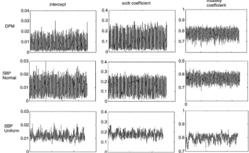
We compared the IUM model with the DPM model and to an SBP with a normal mixture setup. To facilitate inference for both of these alternatives, we adjusted our computation to account for the normal mixture setup. We provide the details of this adjustment in AppendixB. We ran the MCMC sampler under all three setups using 35,000 iterations and discarded the initial 5000 as burn in. Trace plots (Figure 1) and the median es-timates together with the 95% credible intervals of the posterior samples of the volatility parameters, β0, β1,and, φ (Table 1)
were generated.
The trace plots show the mixing of the volatility coefficients under the three Bayesian nonparametric models. It is very sim-ilar for the DPM and SBP-normal, and for the IUM it is also good. The volatility estimates of the IUM model are the ones that are closer to the true values. Though the other two models,
Figure 1. Trace plots of the posterior samples of the volatility coefficients,β0,β1(arch coefficient) andφ(volatility coefficient).
DPM and SBP-normal do well in estimating the value ofφ, they underestimate the values ofβ0 andβ1.Finally the 95%
credi-ble intervals under the DPM and the SBP-normal have similar width whereas those of the IUM model are actually narrower.
To compare the fit of each of the three competing models, we calculated the Mean Integrated Squared Error (MISE). Clas-sically the MISE = (ftrue
ǫ (x)−fˆǫ(x))2dx, wherefǫtrue(x) is the true density of the innovations and ˆfǫ(x) is the estimated density. The model with the smallest MISE is preferred. In our Bayesian approach, MISE is viewed as the posterior expecta-tion of the distance between the true density estimated at pointx
andfǫevaluated atx, that is, E[
(fǫtrue(x)−fǫ(x))2dx|y].We approximate this expectation by
1
M M
it=1
up lo
fǫtrue(x)−fǫ(it)(x)2 dx
,
where it=1, . . . , M is the index of the iterations andf(it)
ǫ is the estimated density at iteration it.We ensure thatFtrue
ǫ (lo)= 10−5andFtrue
ǫ (up)=1−10−5, and evaluate the integral using the trapezoidal rule. The MISE estimates are also displayed in Table 1. From the comparison of the three MISE estimates, it is clear that the IUM has the best fit. These results for both the MISE and the volatility estimates demonstrate the flexibility of the IUM over the two normal setups: the DPM and the SBM-normal. Having a uniform mixture coupled with the ability to control the decay of the weights leads to better fitting models and volatility estimates that are closer to the true values of the model from where the data were generated.
We assessed the predictive performance of the competing models by calculating both average log predictive scores (LPS) and average log predictive tail scores (LPTS; Delatola and Griffin 2011). These scores are based on the one step ahead predictive density f(yt+1|y(1:t−1),ϑ), where ϑ represents the
Table 1. Median estimates of volatility coefficients and MISE with their 95% credible intervals
β0 β1 φ MISE
True value 0.010 0.150 0.800
DPM 0.007 0.105 0.776 0.015
(0.002,0.017) (0.023,0.226) (0.718,0.823) (0.0003,0.1258)
SBP-normal 0.009 0.100 0.777 0.016
(0.003,0.019) (0.042,0.245) (0.727,0.808) (0.0004,0.1176)
IUM 0.011 0.165 0.797 0.007
(0.004,0.015) (0.085,0.219) (0.758,0.824) (0.0043,0.0234)
NOTE: Italics differentiate true parameter values from estimated values.
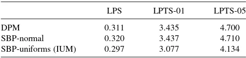
Table 2. LPS and LPTS under the three models for the simulated data
LPS LPTS-01 LPTS-05
DPM 0.311 3.435 4.700
SBP-normal 0.320 3.437 4.710
SBP-uniforms (IUM) 0.297 3.077 4.134
model parameters, ϕ, the vector of the volatility coefficients, andFǫ,the innovation distribution. We approximate the predic-tive density byf(yt+1|y(1:t−1),ϑˆ),where ˆϑrepresents parameter
estimates. Forϕthese are the posterior medians of each volatility coefficient. ForFǫ the point estimate isFǫ(B)=E[Fǫ(B)] for measurable setsB, which is the Bayes’ estimator under squared loss.
For the calculation of LPS and LPTS,t=1, . . . , nrefers to the latter half of the dataset, the evaluation (out of sample) set. The first half is the training (in sample) set, which is used to estimateϕandFǫ.We calculate LPS as
LPS = −1
n n
t=1
logf(yt|y1:(t−1),ϑˆ). (20)
Under this calculation, smaller values of the LPS indicate a better fitting model. In practice, we may be more interested in predicting extreme returns and thus we calculate the LPTS. We identifyzα, the upper 100α% of the absolute values of the stan-dardizedyt. Since we built a conditional model and are interested in the conditional “tails,” we carried out this standardization, to have a measure of the conditional extreme returns. The stan-dardized yt is calculated as y
★ t =
yt
ˆ
ht, where ˆ
ht is an estimate of volatilityht, calculated using the estimates of the volatility coefficients from the evaluation set. We then find1(|y★
t| ≥zα), the number of extreme returns of y★
t. Thus only predictions of returns with absolute value in the upper 100α% of|y★
t|are included in the score. So, LPTS are,
LPTS= −n 1 t=11(|y
★ t|> zα)
n
t=1
1 |y★ t|> zα
×logf(yt|y1:(t−1),ϑˆ). (21)
In our comparisons we looked at the upper 5% and 1% values. The results are displayed in Table 2. The IUM outperforms the other two models both in terms of the LPS and the LPTS. Its lower LPTS values demonstrate that it can predict extreme returns more accurately than the two alternatives.
5. EMPIRICAL EXAMPLES
In this article we look at daily log returns of three stock indices: the S&P 500, FTSE 100, and EUROSTOXX 50. Our samples for each index, respectively, are from: January 3, 1980 to December 30, 1987, January 3, 1997 to March 12, 2009, and June 7, 2002 to March 3, 2009.Figure 2shows the time plots for the daily log returns.Table 3shows the main summary statistics of these returns.
The plots inFigure 2identify periods of sustained high volatil-ity, which we refer to as volatility clusters. The most notable volatility clusters for each index are those near the end of the sampled time period, which are all related to stock
mar-Table 3. Summary statistics
Descriptives S&P 500 FTSE 100 EUROSTOXX 50
Median 0.044 0.031 0.000
St. Dev. 1.130 1.304 1.610
Skewness −4.129 −0.124 0.010
Kurtosis 90.609 (10.147) 8.772 8.929
ket crashes. For the S&P 500, it was the October 1987 crash whereas for the FTSE 100 and EUROSTOXX 50, it was the 2008 crash caused by the collapse of the subprime mortgage market. From the summary statistics displayed inTable 3, we focus on the estimates of kurtosis and skewness. All three sam-ples have high levels of kurtosis. For the S&P 500, estimated kurtosis is nine times higher when the extreme drop in the prices on October 19, 1987 is in the sample than when it is excluded (the kurtosis after the removal of the outlier is 10.147). This extreme observation also impacts on skewness, which increases to−0.022 from −4.129 once the extreme is removed. The es-timated skewness from the EUROSTOXX 50 sample is positive 0.010 rather than negative as it the case with the samples from the other two indices.
We apply our IUM with the GARCH(1,1), GJR-GARCH(1,1), and EGARCH(1,1) representations for the volatility to all three samples. We then compare our re-sults to those from GARCH(1,1), GJR-GARCH(1,1), and EGARCH(1,1) with Student’s-t innovations and skewed Student’s-t innovations. We refer to these models as para-metric models. They were fitted using Matlab’s Econopara-metrics and Kevin Shephard’s Financial Econometrics toolboxes. Both of these toolboxes carry out maximum likelihood estimation (MLE). Further comparisons were made with two SV models with Student’s-tinnovations one without (SV(1)-t), and one with “leverage effect” (SV(1)-t leverage), using the algorithms of Jacquier, Polson, and Rossi (1994,2004). Finally, we compared our IUM model with a DPM model with the same GARCH-type representations for the volatility, the SV-DPM model of Jensen and Maheu (2010), and theπ-DDP model of Griffin and Steel (2006). In all cases, the priors and samplers suggested by the authors are used. We refer to these models as Bayesian non-parametric models. The results for the IUM and DPM models were based on 480,000 runs with the first 20,000 discarded as burn in. The parameters aj, bj of the SBP are generated from the geometric-beta model (described in Section2) with param-etersα1=1, α2=6.For the DPM , the “precision” parameter,
c=1.
5.1 Results
As was the case with the simulated example, we assess the predictive performance of the competing models by calculating both average LPS and LPTS as per Equations (20) and (21). For the LPTS, we again considered the 5% and 1% points. The volatility estimates used to obtainy★
(the standardized yt) for each index were based on the GJR-GARCH(1,1) model with skewed Student’s-tinnovations. We did estimate the volatility using all GARCH-type models, and since the estimates were similar we decided to use those of the GJR-GARCH(1,1) model. The LPS and LPTS scores for each model and each dataset are included inTable 4.
Figure 2. Time plots of observed daily returns.
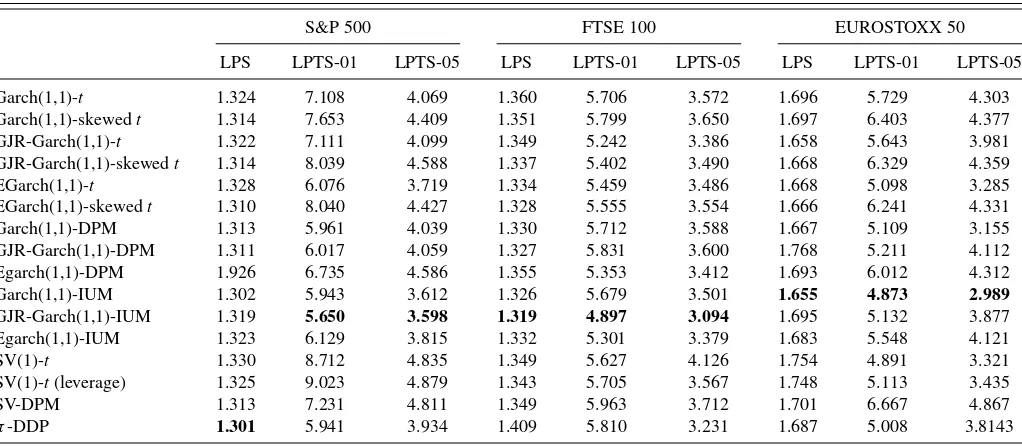
Looking at these scores, we see that the IUM model for the innovation distribution with the three GARCH-type volatility se-tups is a competitive model. It produces the lowest (best) LPS for two of the indices studied, the FTSE 100 and EUROSTOXX 50 and the second best LPS for the S&P 500. In terms of the LPTS, it outperforms all other models for the three indices. Based on the LPTS, both the GJR-IUM and
GARCH(1,1)-IUM have better predictive performance of extreme events when compared with the EGARCH(1,1)-IUM. All the GARCH-type IUM models produce better LPS and LPTS compared with the respective GARCH-type models with DPM innovations and SV-DPM for all indices.
InTable 5, we also provide in-sample estimates of the volatil-ity coefficients for all three sampled indices. For the point
Table 4. Log predictive scores and log predictive tail scores at 1% and 5% for S&P 500, FTSE 100, and EUROSTOXX 50
S&P 500 FTSE 100 EUROSTOXX 50
LPS LPTS-01 LPTS-05 LPS LPTS-01 LPTS-05 LPS LPTS-01 LPTS-05
Garch(1,1)-t 1.324 7.108 4.069 1.360 5.706 3.572 1.696 5.729 4.303
Garch(1,1)-skewedt 1.314 7.653 4.409 1.351 5.799 3.650 1.697 6.403 4.377
GJR-Garch(1,1)-t 1.322 7.111 4.099 1.349 5.242 3.386 1.658 5.643 3.981
GJR-Garch(1,1)-skewedt 1.314 8.039 4.588 1.337 5.402 3.490 1.668 6.329 4.359
EGarch(1,1)-t 1.328 6.076 3.719 1.334 5.459 3.486 1.668 5.098 3.285
EGarch(1,1)-skewedt 1.310 8.040 4.427 1.328 5.555 3.554 1.666 6.241 4.331
Garch(1,1)-DPM 1.313 5.961 4.039 1.330 5.712 3.588 1.667 5.109 3.155
GJR-Garch(1,1)-DPM 1.311 6.017 4.059 1.327 5.831 3.600 1.768 5.211 4.112
Egarch(1,1)-DPM 1.926 6.735 4.586 1.355 5.353 3.412 1.693 6.012 4.312
Garch(1,1)-IUM 1.302 5.943 3.612 1.326 5.679 3.501 1.655 4.873 2.989
GJR-Garch(1,1)-IUM 1.319 5.650 3.598 1.319 4.897 3.094 1.695 5.132 3.877
Egarch(1,1)-IUM 1.323 6.129 3.815 1.332 5.301 3.379 1.683 5.548 4.121
SV(1)-t 1.330 8.712 4.835 1.349 5.627 4.126 1.754 4.891 3.321
SV(1)-t(leverage) 1.325 9.023 4.879 1.343 5.705 3.567 1.748 5.113 3.435
SV-DPM 1.313 7.231 4.811 1.349 5.963 3.712 1.701 6.667 4.867
π-DDP 1.301 5.941 3.934 1.409 5.810 3.231 1.687 5.008 3.8143
NOTE: Models with the best predictive performance are in bold.
Table 5. Estimates of the volatility coefficients for S&P 500, FTSE 100, and EUROSTOXX 50. For the parametric models, the estimates with their 95% confidence intervals are shown. For the Bayesian nonparametric models, the posterior medians with the 95% credible intervals are shown. Note that *** signifies either a standard error virtually close to zero or bounds very close to zero
and hence 95% confidence intervals (or 95% credible intervals) were not calculated. The correlation coefficient estimates for the SV(1)-t with leverage were−0.240,−0.758, and −0.819 for each index, respectively
S&P 500 FTSE 100 EUROSTOXX 50
β0 β1 β2 φ β0 β1 β2 φ β0 β1 β2 φ
Garch(1,1)-t 0.022 0.042 – 0.934 0.011 0.100 – 0.897 0.012 0.084 – 0.912
(0.006,0.038) (0.022,0.062) – (0.903,0.965) (0.003,0.020) (0.078,0.122) – (0.875,0.920) (0.002,0.022) (0.061,0.108) – (0.889,0.936)
Garch(1,1) skewt 0.023 0.043 – 0.932 0.011 0.095 – 0.902 0.012 0.080 – 0.915
(0.022,0.023) (0.0428,0.0432) – (0.931,0.933) (***) (0.0948,0.0952) – (0.9018,0.9022) (0.0116,0.0124) (0.0796,0.0804) – (0.913,0.917)
GJR-Garch(1,1)-t 0.030 0.033 0.035 0.918 0.014 0.001 0.144 0.918 0.017 0.0001 0.156 0.914
(0.01,0.05) (0.009,0.057) (0.002,0.068) (0.883,0.953) (0.008,0.020) (***) (0.111,0.177) (0.898,0.938) (0.009,0.025) (***) (0.111,0.201) (0.889,0.940)
GJR-Garch(1,1) skewt 0.031 0.034 0.035 0.916 0.013 0.0001 0.138 0.922 0.016 0.0001 0.155 0.914
(0.030,0.032) (***) (0.033,0.037) (0.914,0.918) (***) (***) (0.137,0.139) (0.9218,0.9222) (***) (***) (0.154,0.157) (0.9136,0.9144)
Egarch(1,1)-t −0.019 0.176 −0.108 0.910 0.0001 0.122 −0.114 0.985 0.005 0.108 −0.140 0.985
(−0.033,−0.005) (0.115,0.237) (−0.145,−0.071) (0.871,0.950) (***) (0.089,0.155) (−0.138,−0.091) (0.981,0.989) (0.001,0.010) (0.069,0.147) (−0.167,−0.113) (0.981,0.989)
Egarch(1,1) skewt 0.004 0.107 −0.033 0.982 0.003 0.116 −0.112 0.985 0.007 0.104 −0.143 0.985
(***) (0.106,0.108) (−0.0334,−0.0326) (***) (***) (***) (***) (***) (***) (***) (−0.144,−0.142) (***)
Garch(1,1)-DPM 0.013 0.021 – 0.922 0.007 0.061 – 0.899 0.000 0.000 – 0.837
(0.002,0.056) (0.004,0.074) – (0.866,0.952) (0.001,0.016) (0.016,0.106) – (0.866,0.919) (***) (***) – (0.797,0.918)
GJR-Garch(1,1)-DPM 0.032 0.030 0.034 0.900 0.100 0.005 0.012 0.916 0.005 0.000 0.001 0.909
(−0.007,0.119) (0.005,0.079) (0.005,0.115) (0.828,0.937) (0.034,0.162) (0,0.019) (0.003,0.020) (0.890,0.932) (0.001,0.019) (***) (0.000,0.002) (0.876,0.928)
Egarch(1,1)-DPM −0.041 0.137 −0.040 0.978 −0.173 0.188 −0.003 0.985 0.000 0.000 −0.382 0.978
(−0.114,−0.013) (0.061,0.254) (−0.062,−0.001) (0.952,0.990) (−0.308,−0.109) (0.100,0.259) (−0.012,−0.001) (0.978,0.990) (−0.167,0.000) (0.000,0.082) (−0.600,−0.029) (0.965,0.988)
Garch(1,1)-IUM 0.025 0.045 – 0.918 0.003 0.032 – 0.903 0.002 0.012 – 0.920
(0.001,0.176) (0.008,0.095) – (0.851,0.958) (0,0.009) (0.003,0.100) – (0.890,0.915) (0,0.003) (0.009,0.019) – (0.895,0.932)
GJR-Garch(1,1)-IUM 0.060 0.044 0.072 0.890 0.014 0.004 0.111 0.912 0.001 0.0002 0.135 0.926
(0.013,0.150) (0.006,0.108) (0.015,0.126) (0.790,0.920) (0.004,0.024) (0,0.013) (0.030,0.163) (0.902,0.923) (0,0.007) (0,0.002) (0.009,0.165) (0.907,0.941)
Egarch(1,1)-IUM 0.08 0.192 −0.078 0.960 0.0003 0.132 −0.145 0.986 −0.057 0.089 −0.132 0.983
(0.001,0.121) (0.126,0.283) (−0.123,−0.033) (0.917,0.988) (−0.0032,0.0271) (0.082,0.190) (−0.192,−0.099) (0.984,0.989) (−0.102,0.004) (0.029,0.199) (−0.208,−0.040) (0.979,0.989)
SV(1)-t −0.015 – – 0.962 0.00 – – 0.984 0.002 – – 0.988
(−0.029,−0.004) – – (0.934,0.980) (−0.006,0.006) – – (0.976,0.992) (−0.006,0.011) – – (0.979,0.995)
SV(1)-tleverage −0.005 – – 0.984 0.007 – –8 0.985 0.011 – – 0.986
(−0.015,0.002) – – (0.9663,0.996) (0.003,0.012) – – (0.978,0.990) (0.006,0.017) – – (0.981,0.991)
SV(1)-DPM – – – 0.984 – – – 0.989 – – – 0.992
– – – (0.963,0.997) – – – (0.979,0.997) – – – (0.982,0.999)
estimates of the volatility coefficients under the Bayesian mod-els, we calculate the posterior medians and also provide their 95% credible intervals. Theπ-DDP of Griffin and Steel (2006) models the volatility nonparametrically and therefore there are no volatility coefficients to estimate. For the parametric models, we calculate these estimates based on MLE and provide their 95% confidence intervals. Regarding the SV(1)-twith “lever-age,” we do not include a value for a leverage coefficient. The “leverage effect” in this model is estimated by the correlation between the innovations and the noise terms of the volatility. We do provide these values within the caption ofTable 5. The esti-mates ofβ1andφfor the GARCH(1,1) and GJR-GARCH(1,1)
models are not much different under the Student’s-tand skewed Student’s-tchoices for the innovation distribution for all three in-dices. The estimates forφunder the two Bayesian nonparametric settings forFǫ, DPM and IUM, for each GARCH-type model are marginally lower to the those under Student’s-tand skewed Student’s-t innovations. In terms of the IUM model, the esti-mates ofβ1are actually similar whereas that of DPM are lower.
There is some disparity across both parametric and Bayesian nonparametric models when it comes to the leverage coefficient
β2. If we set the parametric models as the benchmarks, then
IUM seems to slightly under estimate for the FTSE 100 and EUROSTOXX 50 and over estimate for the S&P 500, whereas the DPM largely under estimatesβ2for the FTSE 100 and
EU-ROSTOXX 50, but provides a similar estimate for the S&P 500. The EGARCH(1,1) estimates ofβ1 andβ2vary across the
distributional choices for the innovations and across indices, whereas the estimates ofφare more similar. Looking at the es-timates ofφunder the two SV(1)-tmodels and the SV(1)-DPM, we would say that those are close to the corresponding estimates of the EGARCH(1,1) models.
We also provide in-sample estimates of the kurtosis ˆκy t of the unconditional distribution ofyt.We were able to check for the existence of a fourth moment and then proceed to calculate
ˆ κy
t for all GARCH-type setups with the EGARCH(1,1) being the exception. In EGARCH models, the exponential growth of the conditional variance ofytchanges with the level of shocks, which leads to the explosion of the unconditional variance of
ytwhen the probability of extreme shocks is large. This means that the existence of the unconditional variance of yt (in the EGARCH case) depends on the choice of innovations distribu-tion. We have chosen the Student’s-tand skewed Student’s-tto model the innovations in the parametric models and under these two choices the unconditional variance ofytdoes not exist. The formulas used to check for the existence of the fourth moment, and calculate ˆκy
t for the remaining GARCH-type and SV se-tups are included in AppendixC. These formulas were extracted from Jondeau and Rockinger (2003), Carnero-Angeles, Pena, and Ruiz (2004), and Verhoeven and McAleer (2004). All these formulas are based on the estimates of the volatility coefficients, and the estimated kurtosis of the innovation distribution, ˆκǫ.We used the estimates of the degrees of freedom and the skewness parameter (where applicable) to calculate ˆκǫ.For the Bayesian nonparametric GARCH-type models, the IUM and the DPM, the estimated kurtosis of the innovation distributionκǫ is that of the point estimateFǫ(·) ofFǫ. It is not possible to calculate
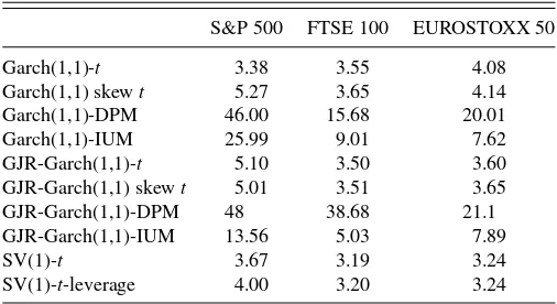
Table 6. Estimates of unconditional kurtosis, ˆκy
t, ofyt. The ***
signify failure to meet the conditions for the existence of a 4th moment, resulting in unbounded kurtosis (see AppendixC)
S&P 500 FTSE 100 EUROSTOXX 50
Garch(1,1)-t 3.71 *** ***
Garch(1,1) skewt 6.27 *** ***
Garch(1,1)-DPM 55.37 49.47 20.01
Garch(1,1)-IUM 85.70 9.63 7.68
GJR-Garch(1,1)-t 6.33 *** ***
GJR-Garch(1,1) skewt 6.19 *** ***
GJR-Garch(1,1)-DPM *** 40.04 21.10
GJR-Garch(1,1)-IUM *** 10.69 ***
SV(1)-t 5.60 8.34 10.94
SV(1)-t-leverage 5.82 7.64 8.65
an estimate of the unconditional kurtosis ofytunder theπ-DDP model of Griffin and Steel (2006) and under the SV(1)-DPM of Jensen and Maheu (2010). For the former model, this is because the volatility is modeled using an ordered dependent DP, and thus no volatility coefficient estimates exist, and for the latter model the innovation distribution is not specified. The estimates of the unconditional kurtosis ofyt are displayed inTable 6and the estimates of the kurtosis of the innovation distribution are displayed inTable 7. There are cases where the relevant con-dition for the existence of a fourth moment was not met and this occurs mostly with the EUROSTOXX 50. For this reason the unconditional kurtosis ofyt is considered unbounded and cannot be estimated. We were however able to calculate ˆκy
t for most models for the other two indices, the S&P 500 and FTSE 100. All GARCH-type models with DPM innovations tend to overestimate ˆκy
t for all indices. For the FTSE 100, we have three estimates that are close to the empirical value, those of the GARCH(1,1)-IUM, GJR-GARCH(1,1)-IUM, and SV(1)-t
(with and without leverage). The estimates of the GARCH(1,1)-IUM model are closest to the empirical values of kurtosis dis-played inTable 3for the S&P 500 and EUROSTOXX 50. These results support our motivation for using the IUM to model the innovation distribution.
Finally, in Table 8 we provide in-sample estimates of the skewness parameterλfor all GARCH-type models with skewed Student’s-t, DPM, and IUM innovations. Overall, the estimates
Table 7. Estimates of the kurtosis of the innovation distribution,κǫ (see AppendixB)
S&P 500 FTSE 100 EUROSTOXX 50
Garch(1,1)-t 3.38 3.55 4.08
Garch(1,1) skewt 5.27 3.65 4.14
Garch(1,1)-DPM 46.00 15.68 20.01
Garch(1,1)-IUM 25.99 9.01 7.62
GJR-Garch(1,1)-t 5.10 3.50 3.60
GJR-Garch(1,1) skewt 5.01 3.51 3.65
GJR-Garch(1,1)-DPM 48 38.68 21.1
GJR-Garch(1,1)-IUM 13.56 5.03 7.89
SV(1)-t 3.67 3.19 3.24
SV(1)-t-leverage 4.00 3.20 3.24
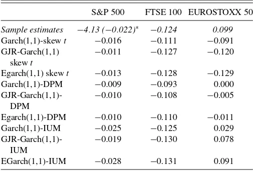
Table 8. Estimates of skewness parameter,λ. Comparisons are for GARCH-type models with skewed-t, DPM, and IUM innovations.
Sample estimates are in italics
S&P 500 FTSE 100 EUROSTOXX 50
Sample estimates −4.13 (−0.022)∗ −0.124 0.099
Garch(1,1)-skewt −0.016 −0.111 −0.091
GJR-Garch(1,1) skewt
−0.011 −0.127 −0.120
Egarch(1,1) skewt −0.013 −0.128 −0.129
Garch(1,1)-DPM −0.009 −0.093 0.000
GJR-Garch(1,1)-DPM
−0.010 −0.108 −0.005
Egarch(1,1)-DPM −0.010 −0.110 −0.011
Garch(1,1)-IUM −0.025 −0.125 0.029
GJR-Garch(1,1)-IUM
−0.019 −0.130 0.078
EGarch(1,1)-IUM −0.028 −0.131 0.091
*In parenthesis: skewness estimate when the extreme outlier is removed.
ofλfor models with IUM innovations are closest to the sample estimates for all indices.
6. CONCLUSIONS
This article introduces a new Bayesian semiparametric model for the conditional distribution of daily stock index returns. The innovation distribution is modeled nonparametrically with an infinite mixture of scaled uniform distributions (IUM) rather than an infinite mixture of normals, as is the case with the DPM. We replaced the normal kernel with the scaled uniform kernel to capture the unimodality, asymmetry, and heavy-tailed be-havior of the conditional return distribution. We used an SBP, instead of a DP prior to model the unknown number of mixture components, because it has the flexibility to generate more com-ponents with nonnegligible weights that could account for the heavy tails of the conditional return distribution. The uniform kernel together with the SBP can absorb extreme returns via the heavy tails and avoid the risk of creating a mode at those extreme points, as may be the case with the DPM model. We de-veloped an efficient MCMC based on the slice-efficient sampler introduced in Kalli, Griffin, and Walker (2011), which samples the volatility coefficients as a block using adaptive MH. In our simulated study based on a GARCH(1,1) model, our IUM has the best fit and predictive performance when compared with the DPM.
We accounted for the “leverage effect” using both a GJR-GARCH(1,1) and an EGJR-GARCH(1,1) and tested our IUM on three samples of daily index returns taken from the S&P 500, FTSE 100, and EUROSTOXX 50. We compared our model with GARCH(1,1), GJR-GARCH(1,1), and EGARCH(1,1) with Student’s-tand skewed Student’s-t, and DPM innovations, and found that its predictive performance in terms of extreme returns is better. It also accounts for kurtosis and skewness more accu-rately. We came to the same conclusion when we compared the IUM with an SV(1) with Student’s-tinnovations (with and with-out leverage), the SV(1)-DMP of Jensen and Maheu (2010), and
π-DDP (Griffin and Steel2006). The over-arching conclusion is that the IUM model developed in this article is competitive and
can lead to improved inferences and predictions in the context of returns data analysis.
APPENDIX A: SPECIFICATION OF SBP PARAMETERS
In Section2, we introduced a method of specifying the pa-rameters (aj, bj) of the SBP for the mixture weightswj. In this appendix, we discuss this method in more detail.
Ifwj ∼SBP(aj, bj), then dition to ensure that F is a random measure, see Ishwaran and James (2001). Asaj/bj =τj/(1−τj) and log(1+τi/(1−
thereforeFis a random measure.
We center this process over a distribution for the weights by choosing E[wj]=ξj,whereξj is Pr(X=j) for a random variableX with a discrete distribution on 1,2,3, . . . .The ran-dom variableX is given a Beta-Geometric distribution, that is, Pr(X=j)=p(1−p)j−1, wherep∼Be(α1, α2).This yields
ξj =
Ŵ(α1+α2)Ŵ(α1+1)Ŵ(α2+j−1)
Ŵ(α1)Ŵ(α2)Ŵ(α1+α2+j)
,
which allows us to control the number of nonnegligible weights by choosing the values of (α1, α2).
To understand how the variance of wj affects the weight decay, we reparameterize aj andbj as aj =rjτj and bj =
The choice ofqj is what controls the variance of wj and de-termines how close in probability the weights are to ξj. We
choose qj to satisfy qj =(1−τj)−1[1−
and hence
One particular idea, which is used in the numerical illustra-tions, is to take large variances, amounting to a noninforma-tive prior. This impliesqj is chosen to be small, but not zero, and hence one could setξjl<j(1−qlτl)−ξj2=cξ, for some smallcξ, for allj. This follows since var(wj)< ξj(1−ξj) and we obtain this limit asqj ↓0.
APPENDIX B: COMPUTATION STEPS WITH NORMAL KERNEL AND NORMAL BASE MEASURE
In both the SBP with normals and DPM case, the hierarchical setup is the geometric-beta model (described in AppendixA) with pa-rametersα1=1, α2=6.
We use the MCMC algorithm described in Section3for all models. For both SBP with the normal setup and DPM, the joint posterior distribution is proportional to
n
Recall that ζ andv are conditionally independent and so the sampling steps are:
The random walk MH described in Section3is used to sample the volatility coefficients. What changes in the case of the nor-mal setup is the likelihood and as a consequence the simplified likelihood used the MH sampler. The likelihood is proportional to
The simplified likelihood is obtained by integrating out theμdt over (−∞,∞) and then theσ2
whereNcis the number of full clusters,nj is the size of cluster
j, and
APPENDIX C: CONDITIONS FOR EXISTENCE OF FOURTH MOMENT FOR THE CALCULATION
OF THE KURTOSIS ESTIMATES
The GARCH(1,1) condition for the existence of a fourth mo-ment is
(β1+φ)2+β12(κǫ−1)<1.
If this condition is satisfied, then the unconditional kurtosis ofyt is
andκǫis the kurtosis of the innovation distribution (see Carnero-Angeles, Pena, and Ruiz2004).
The GJR-GARCH(1,1) condition for the existence of a fourth moment is If this condition is satisfied, then the unconditional kurtosis of
yt is tribution (see Verhoeven and McAleer2004).
In our illustrations, we are using an SV(1) setup for the volatil-ity, that is, logh2t = β0+φlogh2t−1+ηt,whereη∼N(0, ση2). In this case if the kurtosis of the innovations’ distributions,κǫ, is finite, the condition for the existence of the unconditional kurto-sis ofyt,κyt, is the stationarity condition, that is,|φ|<1.Then
(see Carnero-Angeles, Pena, and Ruiz2004).
The formula for calculating the kurtosis of the Student’s-t
distribution is
κǫ=3+ 6
df−4 for df>4,
where df are the degrees of freedom. Calculating the kurtosis of the skewed Student’s-tdistribution is more challenging. As with any distribution, the kurtosis of the innovations’ distribution is given by
We use the formulas in Jondeau and Rockinger (2003) to calcu-late these moments. The formulas are
E(ǫ) = 4λcǫ
andλis the skewness parameter.
ACKNOWLEDGMENTS
Authors thank the referees, the associate editor, and editor for their valuable comments.
[Received June 2010. Revised February 2013.]
REFERENCES
Atchade, Y., and Rosenthal, J. (2005), “On Adaptive Markov Chain Monte Carlo Algorithms,”Bernoulli, 11, 815–828. [375]
Bai, X., Russell, J., and Tiao, G. (2003), “Kurtosis of GARCH and Stochastic Volatility Models With Non-Normal Innovations,”Journal of Econometrics, 114, 349–360. [371]
Bollerslev, T. (1986), “Generalized Autoregressive Conditional Heteroscedas-ticity,”Journal of Econometrics, 31, 307–327. [371,373]
——— (1987), “A Conditionally Heteroskedastic Time Series Model for Spec-ulative Prices and Rates of Return,”Review of Economics and Statistics, 69, 542–547. [371]
——— (2008), “Glossary to ARCH (GARCH),” Technical Report 2008-49, Center of Research in Econometric Analysis of Time Series, School of Economics and Management, University of Aarhus. [371]
Carnero-Angeles, M., Pena, D., and Ruiz, E. (2004), “Persistence and Kur-tosis in GARCH and Stochastic Volatility Models,”Journal of Financial Econometrics, 2, 319–342. [380,382]
Chen, Q., Gerlach, R., and Lu, Z. (2012), “Bayesian Value at Risk and Expected Shortfall Forecasting Via the Asymmetric Laplace Distribution,” Computa-tional Statistics and Data Analysis, 56, 3498–3516. [371]
Chen, C., and So, M. (2006), “On Threshold Heteroscedastic Model,” Interna-tional Journal of Forecasting, 22, 73–89. [375]
Chib, S., and Hamilton, B. (2002), “Semiparametric Bayes Analysis of Longitudinal Data Treatment Models,”Journal of Econometrics, 110, 67–89. [372]
Cont, R. (2001), “Empirical Properties of Asset Returns: Stylized Facts and Statistical Issues,”Quantitative Finance, 1, 223–236. [371]
Delatola, E., and Griffin, J. (2011), “Bayesian Nonparametric Modelling of the Return Distribution With Stochastic Volatility,”Bayesian Analysis, 6, 901–926. [376]
Engle, R. F. (1982), “Autoregressive Conditional Heteroscedasticity With Es-timates of the Variance of U.K Inflation,”Econometrica, 50, 987–1008. [371]
Feller, W. (1957),Introduction to Probability Theory and its Applications(Vol. 1), New York: Wiley. [373]
Ferguson, T. (1973), “A Bayesian Analysis of Some Nonparametric Problems,”
The Annals of Statistics, 1, 209–230. [372]
Fernandez, C., and Steel, M. F. J. (1998), “On Bayesian Modelling of Fat Tails and Skewness,”Journal of the American Statistical Association, 93, 359– 371. [373]
Freedman, D. (1963), “On the Asymptotic Behaviour of Bayes Estimates in the Discrete Case,” Annals of Mathematical Statistics, 34, 1386–1403. [372]
Gallant, A., and Tauchen, G. (1989), “Semi-Nonparametric Estimation of Con-ditionally Constrained Heterogeneous Processes: Asset Prices Application,”
Econometrica, 57, 1091–1120. [371]
Gilks, W. R., and Wild, P. (1992), “Adaptive Rejection Sampling for Gibbs Sampling,”Applied Statistics, 41, 337–348. [374]
Glosten, L., Jagannathan, R., and Runkle, D. (1993), “On the Relation Between the Expected Value and the Volatility of the Nominal Excess Return on Stocks,”The Journal of Finance, 48, 1779–1801. [373]
Griffin, J. E., and Steel, M. F. J. (2006), “Order-Based Dependent Dirichlet Processes,”Journal of the American Statistical Association, 101, 179–194. [372,377,380,381]
Haario, H., Saksman, E., and Tamminen, J. (2001), “An Adaptive Metropolis Algorithm,”Bernoulli, 7, 223–242. [375]
Halmos, P. (1944), “Random Alms,”The Annals of Mathematical Statistics, 15, 182–189. [372]
Hansen, B. E. (1994), “Autoregressive Conditional Density Estimation,” Inter-national Economic Review, 35, 705–730. [371]
Hirano, K. (2002), “Semiparametric Bayesian Inference in Autoregressive Panel Data Models,”Econometrica, 70, 781–799. [372]
Hjort, N. L., Holmes, C., M¨uller, P., and Walker, S. (eds.). (2010),Bayesian Non-parametrics: Statistic and Probabilistic Mathematics(1st ed.), Cambridge: Cambridge University Press. [372]
Ishwaran, H., and James, L. F. (2001), “Gibbs Sampling Methods for Stick-Breaking Priors,”Journal of the American Statistical Association, 96, 161– 173. [372,381]
Jacquier, E., Polson, N., and Rossi, P. E. (1994), “Bayesian Analysis of Stochas-tic Volatility Models,” Journal of Business and Economic Statistics, 12, 371–417. [377]
——— (2004), “Bayesian Analysis of Stochastic Volatility Models With Fat-Tails and Correlated Errors,” Journal of Econometrics, 122, 185– 212. [377]
Jensen, M. (2004), “Semiparametric Bayesian Inference of Long Memory Stochastic Volatility Models,”Journal of Time Series Analysis, 25, 895– 922. [372]
Jensen, M. J., and Maheu, J. M. (2010), “Bayesian Semiparametric Stochastic Volatility Modeling,”Journal of Econometrics, 157, 306–316. [372,377,380,381]
Jondeau, E., and Rockinger, M. (2003), “Conditional Volatility, Skewness and Kurtosis: Existence, Persistence, and Comovements,”Journal of Economic Dynamics and Control, 27, 1699–1737. [380,383]
Kalli, M., Griffin, J., and Walker, S. (2011), “Slice Sampling Mixiture Models,”
Statistics and Computing, 21, 93–105. [374,381]
Kingman, J. (1974), “Random Discrete Distributions,”Journal of the Royal Statistical Society,Series B, 37, 1–22. [372]
Leslie, D., Kohn, R., and Nott, D. (2007), “A General Approach to Heteroscedas-tic Linear Regression,”Statistics and Computing, 17, 131–146. [372] Lo, A. Y. (1984), “On a Class of Bayesian Nonparametric Estimates: I. Density
Estimates,”The Annals of Statistics, 12, 351–357. [372]
Nelson, D. B. (1990), “Stationarity and Persistence in the GARCH(1,1) Model,”
Econometric Theory, 6, 318–334. [371,373]
Poon, S., and Granger, C. (2003), “Forecasting Volatility in Financial Markets: A Review,”Journal of Economic Literature, 41, 478–539. [371]
Roberts, G., Gelman, A., and Gilks, W. (1997), “Weak Convergence and Op-timal Scaling of Random Walk Metropolis Algorithms,”Annals of Applied Probability, 7, 110–120. [375]
Roberts, G., and Rosenthal, J. (2009), “Examples of Adaptive MCMC,”Journal of Computational and Graphical Statistics, 18, 349–367. [375]
Shahbaba, B. (2009), “Discovering Hidden Structures Using Mixture Models: Application to Nonlinear Time Series Processes,” Stud-ies in Nonlinear Dynamics and Econometrics, 13. Available at
http://www.bepress.com/snde/vol13/iss2/art5[372]
Taylor, S. (1982), “Financial Returns Modelled by the Product of two Stochastic Processes – A study of the Daily Sugar Prices 1961–1975,” inTime Series Analysis: Theory and Practice(Vol. 1), ed. O. D. Anderson, Amsterdam: North Holland, pp. 203–226. [371]
Taylor, S. J. (2005),Asset Price Dynamics, Volatility, and Prediction, Princeton, NJ: Princeton University Press. [371]
Theodossiou, P. (1998), “Financial Data and the Skewed Generalized T Distri-bution,”Management Science, 44, 1650–1661. [371]
Tsay, R. S. (2005),Analysis of Financial Time Series: Probability and Statistics
(2nd ed.), Hoboken, NJ: Wiley. [371]
Verhoeven, P., and McAleer, M. (2004), “Fat Tails and Asymmetry in Financial Volatility Models,”Mathematics and Computers in Simulation, 64, 351–361. [380,382]