Full Terms & Conditions of access and use can be found at
http://www.tandfonline.com/action/journalInformation?journalCode=ubes20
Download by: [Universitas Maritim Raja Ali Haji] Date: 11 January 2016, At: 22:18
Journal of Business & Economic Statistics
ISSN: 0735-0015 (Print) 1537-2707 (Online) Journal homepage: http://www.tandfonline.com/loi/ubes20
Constrained Regression for Interval-Valued Data
Gloria González-Rivera & Wei Lin
To cite this article: Gloria González-Rivera & Wei Lin (2013) Constrained Regression for Interval-Valued Data, Journal of Business & Economic Statistics, 31:4, 473-490, DOI: 10.1080/07350015.2013.818004
To link to this article: http://dx.doi.org/10.1080/07350015.2013.818004
View supplementary material
Accepted author version posted online: 12 Jul 2013.
Submit your article to this journal
Article views: 540
Supplementary materials for this article are available online. Please go tohttp://tandfonline.com/r/JBES
Constrained Regression for Interval-Valued Data
Gloria GONZ´
ALEZ-RIVERADepartment of Economics, University of California, Riverside, CA 92521 ([email protected])
Wei LIN
International School of Economics and Management, Capital University of Economics and Business, Beijing 100070, People’s Republic of China (weilin [email protected])
Current regression models for interval-valued data do not guarantee that the predicted lower bound of the interval is always smaller than its upper bound. We propose a constrained regression model that preserves the natural order of the interval in all instances, either for in-sample fitted intervals or for interval forecasts. Within the framework of interval time series, we specify a general dynamic bivariate system for the upper and lower bounds of the intervals. By imposing the order of the interval bounds into the model, the bivariate probability density function of the errors becomes conditionally truncated. In this context, the ordinary least squares (OLS) estimators of the parameters of the system are inconsistent. Estimation by maximum likelihood is possible but it is computationally burdensome due to the nonlinearity of the estimator when there is truncation. We propose a two-step procedure that combines maximum likelihood and least squares estimation and a modified two-step procedure that combines maximum likelihood and minimum-distance estimation. In both instances, the estimators are consistent. However, when multicollinearity arises in the second step of the estimation, the modified two-step procedure is superior at identifying the model regardless of the severity of the truncation. Monte Carlo simulations show good finite sample properties of the proposed estimators. A comparison with the current methods in the literature shows that our proposed methods are superior by delivering smaller losses and better estimators (no bias and low mean squared errors) than those from competing approaches. We illustrate our approach with the daily interval of low/high SP500 returns and find that truncation is very severe during and after the financial crisis of 2008, so OLS estimates should not be trusted and a modified two-step procedure should be implemented. Supplementary materials for this article are available online.
KEY WORDS: Inverse of the Mills ratio; Maximum likelihood estimation; Minimum distance estimator; Truncated probability density function.
1. INTRODUCTION
With the advent of sophisticated information systems, data collection has become less costly and, as a result, massive datasets have been generated in many disciplines. Economics and business are not exceptions. For instance, financial data are available at very high frequencies for almost every asset that is transacted in a public market providing datasets with millions of observations. Marketing datasets offer high granularity about consumers and products characteristics. Environmental stations produce datasets that contain high and low frequency records of temperatures, atmospheric conditions, pollutants, etc., across many regions. Statistical institutes, such as the Census Bureau, collect socioeconomic information about all individuals in a nation. These massive information datasets tend to be released in an aggregated format, either because of confidentiality rea-sons or because the interest of study is not the individual unit but a collective of units. In these cases, the researcher does not face classical datasets, that is,{yi}fori=1, . . . , nor{yt}for
t=1, . . . , T, whereyiorytare single values in the real line, but
data aggregated in some fashion, like interval data [yl, yu] that
offer information on the lower and upper bound of the variable of interest. For example, information about income or net worth comes very often in interval format or low and high prices of an asset in a given day or daily temperature intervals or low/high prices of electronic devices for several stores, etc.
Interval-valued data are also considered symbolic datasets. Within the symbolic approach (Billard and Diday2003,2006), there are several proposals to fit a regression model to
inter-val data. For a review, see Arroyo, Gonz´alez-Rivera, and Mat´e (2011). The simplest approach (Billard and Diday2000) is to fit a regression model to the centers of the intervals of the dependent variable and of the regressors. Further approaches consider two separate regressions, one for the lower bound and another for the upper bound of the intervals, either with no con-straints in the regression coefficients (Billard and Diday 2002) or by constraining both regressions to share the same regres-sion coefficients (Brito2007). In a similar line, Lima Neto and de Carvalho (2008) proposed running two different regressions, one for the center and another for the range of the intervals, with no constraints. None of these approaches guarantees that the fit-ted values from the regressions will satisfy the natural order of an interval, that is, ˆyl ≤yˆu, for all observations. Lima Neto
and de Carvalho (2010) imposed nonnegative constraints on the regression coefficients of the model for the range and solved a quadratic programming problem to find the least squares solu-tion. However, for these constraints to be effective, the range regression must entertain only nonnegative regressors (e.g., re-gressing the range of the dependent variable on the ranges of the regressors), which limit the usefulness of the model.
In this article, we propose a regression model, either for cross-sectional or time series data, that guarantees the natu-ral order of the fitted interval bounds for all the observations in
© 2013American Statistical Association Journal of Business & Economic Statistics October 2013, Vol. 31, No. 4 DOI:10.1080/07350015.2013.818004
473
the sample and for any potential interval forecast based on the model. Within the framework of interval time series (ITS), we specify a bivariate system for the lower and upper bounds of the time series. The observability restrictionyl,t ≤yu,t implies
that the conditional probability density function of the errors is truncated. Under the assumption of bivariate normal errors, the amount of truncation will depend on the variance-covariance matrix of the errors and it will be time-varying because the trun-cation is a function of the difference between the conditional means of the lower and upper bounds. When the observability restriction is severe, that is, the truncation of the bivariate den-sity is substantial, not only the conditional expectations of the errors are different from zero, but also the errors are correlated with the regressors, thus any least-squares estimation (linear or nonlinear) will fail to deliver consistent estimators of the param-eters of the model. We propose a two-step estimation procedure, combining maximum likelihood (ML) and least squares estima-tion, that will deliver consistent estimators. The first step con-sists of modeling the range of the interval, which is distributed as a truncated normal density, to obtain ML estimates of the inverse of the Mills ratio ˆλt−1, which embodies the severity of
the restriction. Only when the restriction is severe, the second step is necessary. This step consists of introducing ˆλt−1 in a
least-squares regression to correct the selection bias imposed by the restriction. However, the estimation in the second step may be plagued with multicollinearity problems because in some in-stances, ˆλt−1is an almost linear function of the regressors. Since
multicollinearity cannot be resolved by dropping some of the regressors, we propose a modified second step by implementing a minimum distance estimator that delivers consistent estimates of all parameters in the model. The advantage of the modified second step is that even when the observability restriction is not severe (ˆλt ≈0 for mostt), we are able to identify all parameters
without much loss in efficiency.
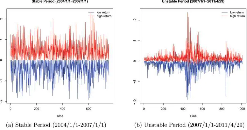
As an illustration of the methods that we propose, we model the interval of daily low/high returns to the SP500 index before and after 2007. Before 2007, the daily interval exhibits very little volatility, but after 2007, volatility is the dominant characteris-tic due to the events of the financial crisis of 2008. These two periods have very different dynamics. We implement the mod-ified two-step estimator and find that in the stable period, the observability restriction is not severe, so simple ordinary least squares (OLS) will suffice to estimate a dynamic system for the lower and upper bounds of the interval. In contrast, in the high volatility period, the restriction is very severe, thus simple OLS estimates should not be trusted and the second step is necessary to guarantee the consistency of the estimators.
The modeling of the low/high interval is interesting in itself for several reasons. For instance, in technical analysis, trading strategies are based on the dynamics of an object, the “candlestick,” which is composed of two intervals, the low/high and the open/close. In financial econometrics, the low/high interval also provides estimators of the volatility of asset returns, see Parkinson (1980); Yang and Zhang (2000); and Alizadeh, Brandt, and Diebold (2002), among others. However, the most important reason for our interest in estimation and forecasting with interval-valued data lies on the fact that the only format available for some datasets is the interval format. Financial datasets are exceptional; they are very rich and information comes in many formats, for example, databases
contain records of prices for every transaction in the market so that we could analyze prices at the highest and the lowest frequencies; there is an almost continuous measurement in the transaction price. But this is not always the case in other areas within economics or in other sciences. Some examples follow.
The U.S. Energy Information Administration gathers elec-tricity prices for each state in the United States. Since there are so many factors affecting the prices of electricity, there is substantial variation across states and across localities in the same state. This agency provides average retail price at the state level in interval format, that is, min/max price, which is more informative of the realities of this market. The U.S. Department of Agriculture provides livestock prices also in interval format. The Livestock Marketing Information Center (Iowa State Uni-versity) reports interval prices of several items, for instance, min/max daily beef prices. Though they compute a weighted price, this is not the price of a given transaction, so the interval min/max contains more valuable information to the participants in the market. In the appraisal industry, the objective is to find a “fair market price” for items, such as real estate, for which the market value cannot be observed directly unless the item is sold. It is standard practice in this industry to record min/max prices of similar items that have had a recent transaction so that the “fair” market price, though nonobservable, must be contained within such an interval. Even with financial datasets, it is interesting to note that bond market data are not as transparent as stock data and bond traders report the bid/ask interval of the transaction, in which the price is contained. In other fields different from eco-nomics, for instance medicine, we have databases with patient data recorded in interval format, the most indicative is blood pressure measurements, that is, diastolic and systolic pressure (low and high numbers, respectively). In earth sciences, temper-ature records across locations also come in interval format, that is, min/max temperature for a given location.
These examples show that the low/high interval of a variable is a common format that provides additional information beyond an average measurement, and in some cases, it is the only format available to the researcher. It should be noted that estimating and forecasting with low/high interval-valued data is different from estimating and forecasting two quantiles. The low/high bounds are extremes. In quantile regression, the loss function requires fixing the probabilityαassociated with the quantile. If we wish to approximate the low/high interval with quantile regression, it seems natural to fixα=0 for the estimation of the lower bound and α=1 for the estimation of the upper bound, but if the variables of analysis are defined in the domain (−∞,+∞), these are also the values of the corresponding (0,1) quantiles. If our interest is any other quantile, for example, the interquartile range [Q0.25, Q0.75], and the data are available
in a classic point-valued format, then quantile regression with monotonicity restrictions could be implemented as proposed by Chernozhukov, Fernandez-Val, and Galichon (2010).
We organize the article as follows. In Section 2, we pro-vide the general framework and basic assumptions. In Section 3, we present the two-step estimation procedure and develop its asymptotic properties. In Section4, we conduct extensive Monte Carlo simulations that show the finite sample properties of the two-step and modified two-step estimators. In Section 5, we compare extensively our methods with those existing in the literature. In Section6, we illustrate the empirical aspects of our
methods with the daily interval of low/high SP500 returns. In Section7, we conclude.
2. GENERAL FRAMEWORK AND BASIC ASSUMPTIONS
We introduce a general regression framework for interval-valued time series. The objective is the estimation of a paramet-ric specification of the conditional mean of an interval-valued stochastic process. Generally, an interval is defined as follows:
Definition 1. An interval [Y] over a set (R,≤) is an ordered pair [Yl, Yu] whereYl, Yu∈Rare the lower and upper bounds
of the interval such thatYl≤Yu.
We can also define an interval random variable on a proba-bility space (, F, P) as the mapping Y :F →[Yl, Yu]⊂R.
In a time series framework, we further define an interval-valued stochastic process as a collection of interval random variables indexed by time, that is,{Yt}fort ∈T, and an interval-valued
time series (ITS) as a realization{[ylt, yut]}Tt=1 of an
interval-valued stochastic process.
We are interested in modeling the dynamics of the pro-cess {Yt} = {[Ylt, Yut]} as a function of an information set
that potentially includes not only the past history of the pro-cess, that is, Yt−1=(Yt−1, Yt−2, . . . , Y0), but also any other
exogenous random variables Xt =(Xt, Xt−1, . . . , X0),where
Xt =(X1t, X2t, . . . , Xpt). In this context, we focus the
mod-eling exercise on establishing the joint dynamics of the lower {Ylt}and upper{Yut}bounds taking into account the natural
or-dering of the interval. Thus, a general data-generating process is written as
Yt≡
Ylt
Yut
=
Gl(Yt−1, Xt;βl)
Gu(Yt−1, Xt;βu)
+
εlt
εut
,
such thatYlt ≤Yut, (2.1)
whereGl(·),Gu(·) are differentiable functions;βl,βuare two
J×1 parameter vectors; andǫt ≡(εlt, εut)′is the error vector.
The observability restrictionYlt ≤Yut will be imposed on the
process.
The observability restriction in (2.1) is the key feature of the specification because it generates two important issues for the estimation of the model (2.1). First, the restriction Ylt ≤Yut
implies a restriction on the distribution of the error vector. The errors now are restricted as follows:
Gl(Yt−1, Xt;βl)+εlt ≤Gu(Yt−1, Xt;βu)+εut,
εut−εlt ≥Gl(Yt−1, Xt;βl)−Gu(Yt−1, Xt;βu).
(2.2)
The transformed observability restriction (2.2) implies that, conditioning on the information setℑt−1≡(Yt−1, Xt), the joint
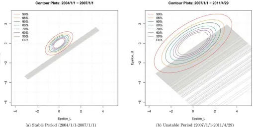
distribution of (εlt, εut) is truncated from below.Figure 1
illus-trates a truncated joint density of the errors. In the plane formed by the variables (εlt, εut), the ellipse represents a contour of the
joint density and the 45◦ degree lineεut=εlt+(Gl−Gu) is
the truncation line, separating the shaded area, whereYlt ≤Yut
holds, from the area where the restriction is violated.
FromFigure 1, we observe that the feasible support for the errors will depend on the error variance-covariance matrix, as
Figure 1. Truncated distribution of the error term. The online ver-sion of this figure is in color.
well as any other parameters affecting the shape of the contours, and on the position of the truncation line, which is a function of the difference between the two conditional mean functions. Small dispersion of the errors together with a large difference, that is,Gl≪Gutend to mitigate the severity of the observability
restriction because it reduces the probability of the errors falling below the truncation line to the point that the restriction might not longer be binding and it could be safely removed from the model. However, if the restriction is binding, it cannot be ignored in the model estimation because, on one hand, it may generate predicted values ofYlt andYut that do not follow the
natural order of an interval, and on the other, it will affect the asymptotic properties of the estimators as we see next. By taking conditional expectations with respect toℑt−1in (2.1),
Et−1(Ylt|Ylt ≤Yut)=Gl(Yt−1, Xt;βl)
+Et−1(εlt|εut−εlt ≥Gl−Gu),
Et−1(Yut|Ylt ≤Yut)=Gu(Yt−1, Xt;βu)
+Et−1(εut|εut−εlt ≥Gl−Gu).
When the observability restriction is binding, the conditional expectations of the errors, which areEt−1(εlt|εut−εlt ≥Gl−
Gu) andEt−1(εut|εut−εlt ≥Gl−Gu), will not be zero, and
furthermore, they will depend on the regressors of the model through the functionsGl(·) andGu(·). Thus, any least-squares
estimation (linear or nonlinear) will fail to deliver consistent estimators for the model.
Before introducing our estimation procedures, we need to state some basic assumptions on (2.1).
Assumption 1 (Weak Stationarity). The interval-valued stochastic process {Yt} = {Ylt, Yut} is covariance stationary,
which means that the lower{Ylt}and upper{Yut}processes are
themselves covariance stationary. We also require covariance stationarity in the regressorsXt ≡(X1t, . . . , Xpt)′.
This assumption allows estimators with standard asymptotic properties. The proposed methods will also apply to nonstation-ary data, but the properties of the estimators will be nonstandard.
Assumption 2 (Exogeneity). The regressors (Yt−1, Xt) are
strictly exogenous variables, that is,E(ǫt|Yt−1, Xt)=0.
This assumption is standard in regression analysis to pro-tect the estimators against endogeneity bias. In our context, the objective is to analyze the dynamics of{Yut}and{Ylt}as a
sys-tem. For instance, in a vector autoregression (VAR) system, the right-hand side of the system will have lags of{Yut}and{Ylt}. If
we were to introduce additional regressorsXt, we could proceed
in several ways, either expanding the VAR system to includeXt
as another element of the system or considering only predeter-mined regressors, that is,Xt−1, Xt−2, . . ., or requiring the weak
exogeneity ofXt. By proceeding in either way, we will focus
exclusively on the endogeneity generated by the binding observ-ability restriction, that is, whenEt−1(εlt|εut−εlt ≥Gl−Gu)
andEt−1(εut|εut−εlt ≥Gl−Gu) are not zero.
Assumption 3(Conditional Independence). (XT, . . . , Xt+1)
and Yt are conditional independent given Xt, that is,
(XT, . . . , Xt+1)⊥Yt|Xt.
This assumption relates to the previous one in the sense that it opens the system of {Yut} and {Ylt} to the effect of other
regressors, which are not explicitly modeled within the system. For instance, in a VAR framework, if we were to model jointly {Yut},{Ylt}, andXt, this assumption will not be needed. But
because we focus only on the dynamics of{Yut}and{Ylt}, we
need to assume that Yt does not Granger-cause Xt to avoid
biased and potentially inconsistent estimators.
Assumption 4 (Normality). The error terms ǫt ≡(εlt, εut)
are iid bivariate normal random variables with joint den-sity f(ǫt)=(2π)−1||−1/2exp{−ǫt′−1ǫt/2} with the 2×2
variance-covariance matrix=[σ2
l ρσlσu;ρσlσu σu2].
This assumption may seem restrictive, but it provides at least a quasi-ML approach to the estimation of {Yut}and {Ylt}. If
the observability restriction is not binding, estimation by ML under normality or by least squares will produce consistent but inefficient estimators. If heteroscedasticity is present, the es-timators are still consistent but we would need to implement a heteroscedasticity-consistent estimator of the variance for a correct inference. If we were to assume any other density, and again running the risk of a false assumption, we would not be sure whether quasi-maximum likelihood estimate results hold (Newey and Steigerwald1997). If the observability restriction is binding, bivariate normality implies that the distribution of the errors is conditionally truncated normal with conditional heteroscedasticity. Our estimation procedures take care of the heteroscedasticity, and since we are modeling extremes, low and high, the density of these variables cannot be symmetric, thus the truncation takes care of the asymmetry. Furthermore, the simulations presented in Sections4and5show that our es-timators are very robust to misspecification of the density when there are relevant dynamics in the conditional means of{Yut}and
{Ylt}. The potential misspecification of the regressorλt−1seems
to affect mainly the estimation of the constant, but we will show that the estimation of the system generates good fitted intervals with substantially smaller losses than other competing methods.
3. ESTIMATION
Given the implications of the observability restriction for a least squares estimator of the parameters in (2.1), it is natural to think that a full information estimator, like ML, will be better
suited to guarantee consistency. In this section, we will intro-duce the conditional log-likelihood function of a sampleyT to
underline the contribution of the restriction to the estimation. However, our main objective is to develop a two-step estima-tion procedure that delivers consistent estimators but is easier to implement and overcomes some of the limitations of the ML estimator.
3.1 Conditional Log-Likelihood Function
For a sample of size T, yT
≡(yT, . . . , y1) and xT ≡
(xT, . . . , x1), and for a fixed initial valuey0, letfY(yT|xT;θ) be
the joint conditional density ofyT, where θ
∈ is an open
where fYt is the density of Yt conditional on the information (Yt−1, Xt). In (3.1), we have also called Assumption 3.
Un-der Assumption 4, the conditional log-likelihood function of a sampleyT is
in which (·) is the standard normal cumulative distribution function.
The ML estimatorθML is the maximizer of (3.2). This
es-timator will be highly nonlinear, even for a linear system as in (2.1), because of the contribution of the observability re-striction term Rt(yt−1, xt;θ) to the log-likelihood function.
Rt(yt−1, xt;θ) provides the probability mass that is left in
the joint density after the truncation takes place. It is eas-ily seen that 0≤Rt(yt−1, xt;θ)≤1. If the restriction is not
binding,Rt(yt−1, xt;θ)=1 for allt, and its contribution to the
log-likelihood function is zero.1In this case, the restriction is redundant and it can be removed from the specification of the model. On the other hand, if the observability restriction is bind-ing that is,Rt(yt−1, xt;θ)<1 for somet, it must be taken into
1A sufficient and necessary condition for a nonbinding restriction is Gl(yt−1,xt;βl)−Gu(yt−1,xt;βu)
σ2
u+σl2−2ρσuσl
≪0 for allt.
account in the estimation of the model. Ignoring the restriction will result in the inconsistency of ML estimator. In theory, the ML estimator has obvious advantage. If the true distribution of εt is normal as in Assumption 4, under certain regularity
conditions, the ML estimatorθMLis consistent and
asymptot-ically normal.2However in practice, given the nonlinearity of the ML estimator induced by the observability restriction, we should expect multiple local maxima in the log-likelihood func-tion leading to multiple solufunc-tions and nontrivial convergence problems in the maximization algorithm. Thus, the consistency of ML estimator will depend on a good guess of the initial value of the parameters. For these reasons, we propose a two-step procedure that combines ML and least squares estimation, is easy to implement, and will deliver consistent estimators of the parameters of the model.
3.2 Two-Step Estimation: General Remarks
Given the popularity of VAR models, we will consider process (2.1) to follow a linear autoregressive specification of orderp. However, the two-step procedure to be described next will be also applicable to nonlinear models by properly choosing a nonlinear estimation technique in the second step.
The interval autoregressive model with p periods lags, IAR(p), is described as follows
with observability restriction ylt ≤yut, and an error term ǫt
that is bivariate normal iid. Conditioning on the information set ℑt−1=(yt−1, . . . , yt−p, . . .), the conditional mean of the
Under the normality Assumption 4, we derive the condi-tional expectation of the errors (see the online Appendix), which are Et−1(εlt|yut ≥ylt)=Clλt−1 and Et−1(εut|yut≥
2Regularity conditions that guarantee the consistency and asymptotic normality of ML estimatorθMLare in Amemiya (1985, theorems 4.1.1 and 4.1.3) and in White (1994, theorem 4.6).
(yt−1, β)≡Gl−Gu=βc+
Therefore, the regression models can be explicitly written as
ylt =βlc+
tingale difference sequences with respect to ℑt−1, that is,
Et−1(vlt|yut ≥ylt)=0 andEt−1(vut|yut ≥ylt)=0.
Two remarks are in order. First, since Cu−Cl=σm, we
need σm>0 to be strictly positive for Cu andCl to be well
defined. This implies that the specific caseσ2
u =σl2andρ =1
must be ruled out. This could happen when the interval [εlt, εut]
is degenerate and collapses to a single value. Second, λt−1 is
the inverse of the Mills ratio and embodies the severity of the observability restriction. When the restriction is nonbinding, Rt(yt−1, xt;θ)=1 for all t, which implies that λt−1=0 for
allt.
Based on regressions (3.5) and (3.6), the two-step estima-tion strategy consists of estimatingλt−1first and assessing how
binding the observability restriction is. The second step is only meaningful when the restriction is binding. In this case, we proceed to plug in ˆλt−1 in (3.5) and (3.6) and perform least
squares. The proposed two-step estimation strategy resembles Heckman’s (1979) two-step procedure for sample selection models. However, there are important conceptual differences. In Heckman’s, the selection mechanism (the first step) includes the full sample of observations, for example women who par-ticipate and who do not in the labor market, and the regression model (the second step) includes a partial sample, those for which the dependent variable of interest is observed, for exam-ple the wage of those women who work. In our strategy, we carry the same sample in both steps because those observations that violate the observability restriction will never be observed. Hence, from the start, our first step will focus on a truncated normal regression that arises very naturally when we model the range of the interval, and from which we will estimate λt−1.
Our second step is analogous to Heckman’s in that the objective is to correct the selection bias of the least-squares estimator in the regression of interest. However, Heckman’s bias is inconse-quential when the error terms of the selection equation and of the regression of interest are uncorrelated. In our second step,
even if the errors of the lower and upper bound regressions are uncorrelated, the inconsistency of the least-squares estimator will remain when the observability restriction is binding and is omitted in the second-step regression.
3.3 Two-Step Estimation: The First Step
Our objective is to estimateλt−1. To this end, we model the
range of the interval yt =yut−ylt, which according to the
IAR(p) model will exhibit the following dynamics
yut−ylt = −
Under normality Assumption 4, and imposing the observability restriction, the difference of the two error terms,εt, follows a
truncated normal distribution. Thus, the conditional density of ytis
Based on (3.8), we can construct the log-likelihood function of a sample ofTobservationsy
T−1L(y;β, σm)
m)]. The ML estimators will be
plugged in (3.3) to finally obtainλt−1.
There are two advantages in modeling the range of the in-terval. The number of estimated parameters is reduced from 2(1+2p)+3 in the full ML estimation (3.2) to 1+2p+1 in (3.9). More importantly, for the truncated normal regression, there is a unique solution to the maximization problem so that the ML estimator is the global maximizer of the likelihood function. Consistency and asymptotic normality of the ML estimators and
ˆ
λt−1are easily established. We add the following assumption.
Assumption 5. (Mixing Conditions) The interval-valued stochastic process{Yt} = {Ylt, Yut}is either (a)φ-mixing of size
−r/(2r−1), r≥1 or (b)α-mixing of size−r/(r−1), such that E|Ylt|r+δ < <∞ and E|Yut|r+δ < <∞ for some
δ >0 for allt.
Theorem 1. (Consistency and Asymptotic Normality of the first-step ML Estimator) Let θ∗≡(β/σm, σm)≡(β∗, σm) be a 1×(2p+2) parameter vector corresponding to model (3.7). Under Assumptions 1–5, the ML estimatorθ∗ has the
ML is asymptotically normally distributed, that is
√
→N(0,V), where the asymptotic covariance matrix isV= −plimT→∞[E(∂2L/∂θ∗∂θ∗′|θ∗
0)] −1.
The truncated normal regression model has been extensively studied for cross-sectional data. Tobin (1958) proposed the ML estimator and Amemiya (1973) proved its consistency and asymptotic normality. Orme (1989) and Orme and Ruud (2002) proved that the solution to the likelihood equations is unique and that there is a global maximizer of the log-likelihood function. The proofs of the asymptotic properties in Amemiya (1973) are directly applicable to time series data by strengthening the moment conditions. With Assumption 5, we replace the Kolmogorov’s strong law of large numbers and Liapounov’s central limit theorem for nonidentically distributed random vari-ables in Amemiya (1973) with McLeish (1974)’s strong law of large numbers (Theorem 2.10) and Wooldridge-White’s (1988) central limit theorem for mixing processes (Corollary 3.1) to guarantee that Theorem 1 holds. The asymptotic properties of the estimator of the inverse of the Mills ratio follow as a corol-lary of Theorem 1 becauseλ(·) is a continuous and differentiable function with respect toθ∗.
Corollary 1. (Consistency and Asymptotic Normality of the Inverse of the Mills Ratio) The estimator of the inverse of the Mills ratio≡(ˆλ0, . . . ,λˆT−1) has the following properties:
(a) λ(yt,β∗
ML) converges in probability to the true
λ(yt, β0∗), that is,λ(yt,β∗ML)−→p λ(yt, β0∗); (b) is asymptotically normally distributed, that is, √T
(−)−→d N(0,S0), where the asymptotic covariance
3.4 Two-Step Estimation: The Second Step
We plug the estimateλt−1 in the regressions (3.5) and (3.6)
to obtain the feasible model. We need to redefine the new error terms in the feasible regressions as ult and uut, which
have two sources of variation, one coming from the λ es-timator, and the other coming from the error term in the infeasible regression, that is, ult =Cl(λt−1−λt−1)+vlt and
uut =Cu(λt−1−λt−1)+vut. As a result, the error term of the
feasible regression will be heteroscedastic. Writing the feasible regressions in matrix form
The least-squares estimators of the parametersγlandγuare
γl =(H′H)−1H′yl, γu=(H′H)−1H′yu. (3.11)
The next theorem establishes the asymptotic properties of the two-step estimatorsγlandγu.
Theorem 2. (Consistency and asymptotic normality of the second-step OLS estimator) Under the following assumptions:
(i) plimT→∞H′H/T =B−1, which is nonsingular;
(ii) H′J(β∗)/T converges uniformly in probability to the matrix function Q(β∗);J′(β∗)J(β∗)/T is bounded uniformly in probability at least in a neighborhood of true valueβ∗
(a) converge to their true values in probability,
(b) with asymptotic normal distributions, that is, √T (γl−γl)
are the variance–covariance matrices of the errorsvlt andvut,
respectively, ifwere observable. The second term Q′
0S0Q0
captures the uncertainty induced by the estimates of. The last two terms,Ml0 andMu0, capture the covariances between the
error termsvlt andvut with. Although vlt andvut are
mar-tingale difference sequences, they are correlated withλt+i for
i=0,1, . . . , T −t. This is a further difference with Heckman’s two-step estimator. In Heckman’s covariance matrix, the matrix
M0 is zero because in a cross-sectional setting the errorvis
uncorrelated with the inverse of the Mills ratio. Since the asymp-totic variance–covariance matrices in (3.12) and (3.13) cap-ture the heteroscedasticity induced by the observability restric-tion together with the time dependence induced by, Newey
and West’s (1994) HAC variance–covariance matrix estimator should suffice to estimate BlB and BuB consistently. We
also estimate the unconditional variancesσ2
l andσu2of the
re-spective errorsεlt andεut and their correlation coefficientρby
implementing a simple method of moments based on the results of Nath (1972) (see the online Appendix).
3.5 Two-Step Estimation: Implementation Issues
The implementation of the two-step estimator may be subject to multicollinearity, and consequently the parameters γl and
γu in the second step, Equation (3.10), may not be precisely
estimated or, in extreme cases, they may not be identified at all. There are two reasons for multicollinearity. First, the functional form (3.3) of the inverse of the Mills ratioλ(·) is nearly linear over a wide range of its argument(yt−1, β)/σ
mso that the
estimated regressor is almost collinear with the regressors inZ. These multicollinearity issues cannot be resolved by just dropping some of the regressors because the inclusion of is necessary to guarantee the consistency of the estimators ˆβl
and ˆβu.
The second reason pertains to those cases in which the ob-servability condition is not binding. When the obob-servability con-dition is not binding, the population value ofλ(·) is zero. Within a sample, we will observe values close to zero and very small variance in ˆλt. The direct consequence is thatClandCuare not
identifiable. In the simulation Section, we will discuss cases in which this problem is severe.
For these two reasons, we propose amodifiedsecond-step es-timator that overcomes the identification problem ofClandCu,
and in addition, provides a direct identification of the uncondi-tional variancesσ2
l andσ 2
u of the respective structural errorsεlt
andεutand their correlation coefficientρ.
3.6 Two-Step Estimation: A Modified Two-Step Estimator
The first step of the estimation is identical to that explained in Section3.3, from which we obtain the estimatesandσm.
In the second step, we exploit the relationships amongCl,Cu,
σu2, andσl2, that is,
would have a unique solution, andClandCuwill be uniquely
identified. By writing σ2
u andσ
2
l as functions of Cl andCu,
that isσu2(Cu) andσl2(Cl), we propose the following minimum
distance estimator, which permits identifyingClandCu,
(Cl,Cu)=arg min
that theunconditionalvarianceσ2
u andσl2of the error termsεut
andεlt can be written as
so that we need consistent estimators for the population mo-mentsE(var(vlt|yt−1)),E(var(vut|yt−1)),andE(var(vt|yt−1))
to obtainσ2
u(Cu) andσl2(Cl) as functions of sample information.
Proposition 1 guarantees that this is the case. First, let us call
Proposition 1. Under Assumptions 1–5 and for φ- or α-mixing sequences vlt and vut with at least finite second
moments, we have that Tt=1v2t/T →−p E(var(vt|yt−1)),
The implementation of the minimum distance estimator in (3.15) is described inFigure 2. 4. calculate the intercept (σ2
u(Cu∗)−σl2(Cl∗))/σm to obtain the
6. go back to 1. Repeat until the distance function (3.15) is minimized by the minimizer (Cl,Cu).
Given the optimal solution (Cl,Cu), the estimators of the
parameters β of the original model are readily available as well as the variance–covariance matrix of the errorsεlt andεut,
Figure 2. Minimum distance estimator.
that is
Theorem 3. (Consistency of Modified Two-Step Estimator) The modified two-step estimator (Cl,Cu) and those defined in
(3.22) converge in probability to the true values of the parame-ters.
To prove Theorem 3, which states the consistency of estimates
Cl andCu in (3.15), we only need to verify the assumptions
stated in Theorem 7.3.2 in Mittelhammer, Judge, and Miller (2000) that guarantee the consistency of extremum estimators.3 Proposition 1 shows that the restricted objective function in (3.15) converges in probability to that provided in (3.14). In addition, since the system of equations (3.14) has a unique solu-tion and the restricted objective funcsolu-tion (3.15) is a continuous and convex function inCl andCu, it is uniquely minimized at
the true values ofClandCu.
4. SIMULATION
We perform Monte Carlo simulations to assess the finite sam-ple performance of the two proposed estimation strategies: the two-step and modified two-step estimators; and compare these
3See Newey and MacFadden (1994, pp. 2133–2134) for the proof. The four assumptions are (a)m(θ,Y,X) converges uniformly in probability to a function ofθ, saym0(θ); (b)m0(θ) is continuous inθ; (c)m0(θ) is uniquely maximized at the true valueθ0; and (d) the parameter spaceis compact.
estimators with a naive OLS estimator that does not take into account the observability restriction.
The data-generating process (DGP) is specified as an IAR(1)
and with an error term that is bivariate normally distributed ǫt ≡(εl,t, εu,t)′∼N(0,).
The ITS{[yl,t, yu,t]}Tt=1is generated sequentially to guarantee
that the bounds are not crossing each other that isyl,t> yu,t.
We proceed as follows. Given the interval datum [yl,t−1, yu,t−1]
at time t−1, we draw error terms ǫt =[εl,t, εu,t] from the
bivariate normal density and calculate [yl,t, yu,t] for timet. If
a cross-over happens (i.e.,yl,t > yu,t), we draw another pair of
error terms until the observability restrictionyl,t ≤yu,tis met. In
doing so, we guarantee that the errorsǫtare truncated bivariate
normally distributed, and that the truncation varies across time because it depends on the past interval-valued data [yt−1] as
well as on the assumed parametersβ’s in the IAR(1) DGP. We have designed eight different specifications inTable 1. We have simulated a block of four DGPs where the observability restriction is binding and another block of four DGPs where it is not. Since the observability restriction for the IAR(1) implies thatǫt/σm≥(yt−1, θ∗), the right-hand side of the inequality
will determine whether the observability restriction is binding or not. We guarantee that the observability restriction is not binding when(yt−1, θ∗)=βc∗+β1∗yl,t−1+β2∗yu,t−1≪
0. Otherwise, the restriction could be mildly or severely binding depending upon the choices of the parameters of the DGP. In our simulations, we fix the parameters inβ1∗andβ2∗and play with the interceptβc∗ to allow the restriction to be binding or not. For the four cases, B-1 to B-4,βlc−βuc =0, so that
the observability restriction becomes binding; and for the four cases, NB-1 to NB-4, βlc−βuc = −4, so that the restriction
is not severely binding. Within each block, we simulate two IAR(1) DGPs, one with high persistence and another with low persistence; and for each one we assume two different variance– covariance matrices for the errors, one with uncorrelated
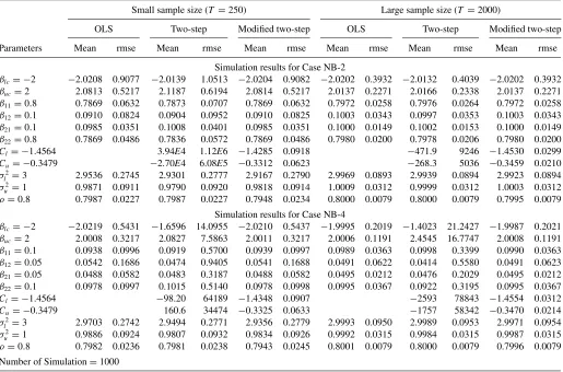
errors and another with highly correlated errors. For each DGP, we also run small and large sample experiments (T =250 and 2000) with 1000 replications per DGP. Due to space constraints, we report here our results for only four cases, B-2 and B-4 in Table 2 and NB-2 and NB-4 in Table 3; the results for the remaining cases are in the the online Appendix. These are our findings for all eight cases:
1. When the observability restriction is binding (Cases B-1 to B-4), the mean values of the OLS estimates are quite far from the true values, as we expected. OLS estimators are not consistent due to the correlation of the regressors with the errors. When the restriction is not severely binding (Cases NB-1 to NB-4), the mean values of the OLS esti-mates are very close to the true values. In this case,λt−1 is
very close to zero, so that the endogeneity problem does not arise.
2. When we implement the two-step estimation, the main is-sue that we face is identification of the model whether or not the restriction is binding. If the restriction is binding but λt−1 is almost linear in the regressors of the model,
multi-collinearity arises (Cases B-3 and B-4). The problem is more severe when there is low persistence in the model and the errors are correlated (Case B-4). Only whenλt−1 exhibits
substantial variation (Cases B-1 and B-2), we do not face a problem with the identification of the model and the mean values of the two-step estimates are very close to the true values. If the restriction is not binding, we expect severe multicollinearity. In Cases NB-1 to NB-4, the root mean squared errors (RMSEs) ofClandCuexplode regardless of
the persistence of the model and the sample size. When there is low persistence in the model (Cases NB-3 and NB-4), the RMSE’s ofβl,c andβu,c also explode because the
nearly-zero regressor λt−1 is highly collinear with the constant
terms.
3. Modified two-step estimation resolves very nicely the iden-tification problem whether the observability restriction is binding or not. If it is binding (Cases B-1 to B-4), the esti-mators are consistent whether there is low or high persistence and whether the errors are or not correlated. The modified two-step estimates are very close to the true values and their
Table 1. Specification of data-generating processes for simulation
Binding cases Nonbinding cases
Parameters B-1 B-2 B-3 B-4 NB-1 NB-2 NB-3 NB-4
βlc 0 0 0 0 −2 −2 −2 −2
Sample size 250, 2000 250, 2000 250, 2000 250, 2000 250, 2000 250, 2000 250, 2000 250, 2000
Number of simulations=1000
Table 2. Simulation results for Cases B-2 and B-4
Small sample size (T =250) Large sample size (T =2000)
OLS Two-step Modified two-step OLS Two-step Modified two-step
Parameters Mean rmse Mean rmse Mean rmse Mean rmse Mean rmse Mean rmse
(a) Simulation results for Case B-2
βlc=0 −1.0645 1.0813 −0.1282 1.2306 −0.0936 0.3890 −1.0054 1.0075 −0.0162 0.3819 −0.0115 0.1312 βuc=0 −0.2738 0.3026 −0.0338 0.8377 −0.0476 0.1658 −0.2448 0.2487 −0.0050 0.2442 −0.0076 0.0544 β11=0.8 0.4648 0.3531 0.7542 0.3869 0.7643 0.1540 0.4852 0.3173 0.7948 0.1247 0.7963 0.0539
β12=0.1 0.4188 0.3430 0.1263 0.4018 0.1171 0.1744 0.4125 0.3157 0.1022 0.1281 0.1006 0.0619
β21=0.1 0.0253 0.1000 0.1002 0.2587 0.0951 0.0718 0.0247 0.0789 0.0999 0.0787 0.0990 0.0256
β22=0.8 0.8602 0.0980 0.7842 0.2655 0.7899 0.0832 0.8731 0.0780 0.7976 0.0800 0.7987 0.0292
Cl = −1.4564 −1.3899 1.8628 −1.4373 0.1344 −1.4505 0.5331 −1.4563 0.0478
Cu= −0.3479 −0.3609 1.3450 −0.3354 0.0778 −0.3523 0.3541 −0.3475 0.0280
σ2
l =3 2.1280 0.8944 2.9323 0.3818 2.9509 0.4000 2.1494 0.8536 3.0014 0.1448 3.0008 0.1431 σ2
u =1 0.9424 0.1009 0.9832 0.0944 0.9858 0.0940 0.9509 0.0576 0.9991 0.0343 0.9993 0.0343 ρ=0.8 0.8268 0.0336 0.8003 0.0291 0.7956 0.0301 0.8270 0.0279 0.8002 0.0102 0.7997 0.0103
(b) Simulation results for Case B-4
βlc=0 −1.1702 1.1777 −85.30 5807 −0.0269 0.5277 −1.1628 1.1638 239.3 5441 0.0035 0.1729 βuc=0 −0.2769 0.2948 −5.8502 3420 −0.0073 0.1732 −0.2782 0.2805 102.5 6127 −0.0010 0.0605 β11=0.1 0.0498 0.1378 −0.0606 8.3845 0.0659 0.2514 0.0572 0.0609 0.2017 8.2371 0.0957 0.0863
β12=0.05 0.0931 0.1799 0.3443 12.6523 0.0723 0.3470 0.0919 0.0720 0.0461 9.9632 0.0538 0.1158
β21=0.05 0.0399 0.0949 −0.1618 6.4568 0.0438 0.1092 0.0391 0.0341 0.0276 7.0154 0.0483 0.0368
β22=0.1 0.1051 0.1260 0.2913 10.9189 0.0999 0.1480 0.1098 0.0446 0.1642 7.1917 0.1007 0.0499
Cl = −1.4564 124.2 7062 −1.4326 0.2111 −318.0 7340 −1.4552 0.0746
Cu= −0.3479 15.77 4069 −0.3380 0.1019 −132.8 8371 −0.3459 0.0388
σ2
l =3 1.6612 1.3476 2.1295 0.8977 2.9675 0.6387 1.6664 1.3349 2.1328 0.8711 3.0002 0.2209 σ2
u =1 0.9213 0.1150 0.9438 0.1060 0.9955 0.1090 0.9224 0.0830 0.9484 0.0605 0.9981 0.0393 ρ=0.8 0.8607 0.0631 0.8274 0.0367 0.7991 0.0367 0.8595 0.0598 0.8270 0.0284 0.7990 0.0137 Number of simulation=1000
standard errors are smaller than those of the two-step esti-mates, even in those cases where the model is well-identified (Cases B-1 and B-2). If the restriction is not binding (Cases NB-1 to NB-4) and thus redundant, the OLS estimator is consistent and efficient but the modified two-step estimator does not seem to be less efficient as the RMSEs of the mod-ified two-step estimates are very close to those of the OLS estimates.
In practice, we do not know a priori whether the restriction is binding. In the first step, we assess the severity of the restric-tion by testing whetherλt =0. In the second step, we gather
further information about the value of the restriction because when it is binding, the OLS estimates should be substantially different from the two-step estimates. In addition, the regres-sorλt−1should be statistically significant. Since
multicollinear-ity affects the significance ofλt−1, we strongly recommend
running the modified two-step estimator and assessing the dif-ferences with the OLS estimator.
5. COMPARISON WITH EXISTING APPROACHES
We compare our two-step (TS) and modified two-step (MTS) estimators with those proposed in the current literature. We implement the approach of Lima Neto and De Carvalho (2008, 2010), henceforth LNC, and we also estimate a location-scale model from which we construct interval estimates.
For an interval-valued time series{Yt} = {[Ylt, Yut]}, we
ob-Their center/range method (CRM) estimates each equation by least squares and their constrained center/range method (CCRM) imposes the restriction βr
j ≥0, j =0, . . . , p on the
equation of the radius to ensure that ˆyrt ≥0 and, therefore,
ˆ
ylt ≤yˆut. Then, the equation of the center is estimated by least
squares and the constrained equation of the radius by adapting Lawson and Hanson’s algorithm.
Before we proceed with the comparison among methodolo-gies, it is very important to underline the implications of the LNC system of center/radius equations for the system of lower/upper bound equations. It is easy to transform the center/radius vec-tor to the lower/upper bound vecvec-tor by defining the 2×2 matrix M=[1/2 1/2 ;−1/2 1/2] such that [yct yrt]′=
M[ylt yut]′. Hence, the system (5.1) and (5.2) is transformed
into a system of lower/upper bounds equations as follows:
Table 3. Simulation results for Cases NB-2 and NB-4
Small sample size (T =250) Large sample size (T =2000)
OLS Two-step Modified two-step OLS Two-step Modified two-step
Parameters Mean rmse Mean rmse Mean rmse Mean rmse Mean rmse Mean rmse
Simulation results for Case NB-2
βlc= −2 −2.0208 0.9077 −2.0139 1.0513 −2.0204 0.9082 −2.0202 0.3932 −2.0132 0.4039 −2.0202 0.3932 βuc=2 2.0813 0.5217 2.1187 0.6194 2.0814 0.5217 2.0137 0.2271 2.0166 0.2338 2.0137 0.2271 β11=0.8 0.7869 0.0632 0.7873 0.0707 0.7869 0.0632 0.7972 0.0258 0.7976 0.0264 0.7972 0.0258
β12=0.1 0.0910 0.0824 0.0904 0.0952 0.0910 0.0825 0.1003 0.0343 0.0997 0.0353 0.1003 0.0343
β21=0.1 0.0985 0.0351 0.1008 0.0401 0.0985 0.0351 0.1000 0.0149 0.1002 0.0153 0.1000 0.0149
β22=0.8 0.7869 0.0486 0.7836 0.0572 0.7869 0.0486 0.7980 0.0200 0.7978 0.0206 0.7980 0.0200
Cl= −1.4564 3.94E4 1.12E6 −1.4285 0.0918 −471.9 9246 −1.4530 0.0299
Cu= −0.3479 −2.70E4 6.08E5 −0.3312 0.0623 −268.3 5036 −0.3459 0.0210 σ2
l =3 2.9536 0.2745 2.9301 0.2777 2.9167 0.2790 2.9969 0.0893 2.9939 0.0894 2.9923 0.0894 σ2
u =1 0.9871 0.0911 0.9790 0.0920 0.9818 0.0914 1.0009 0.0312 0.9999 0.0312 1.0003 0.0312 ρ=0.8 0.7987 0.0227 0.7987 0.0227 0.7948 0.0234 0.8000 0.0079 0.8000 0.0079 0.7995 0.0079
Simulation results for Case NB-4
βlc= −2 −2.0219 0.5431 −1.6596 14.0955 −2.0210 0.5437 −1.9995 0.2019 −1.4023 21.2427 −1.9987 0.2021 βuc=2 2.0008 0.3217 2.0827 7.5863 2.0011 0.3217 2.0006 0.1191 2.4545 16.7747 2.0008 0.1191 β11=0.1 0.0938 0.0996 0.0919 0.5700 0.0939 0.0997 0.0989 0.0363 0.0998 0.3399 0.0990 0.0363
β12=0.05 0.0542 0.1686 0.0474 0.9405 0.0541 0.1688 0.0491 0.0622 0.0414 0.5580 0.0491 0.0623
β21=0.05 0.0488 0.0582 0.0483 0.3187 0.0488 0.0582 0.0495 0.0212 0.0476 0.2029 0.0495 0.0212
β22=0.1 0.0978 0.0997 0.1015 0.5140 0.0978 0.0998 0.0995 0.0367 0.0922 0.3195 0.0995 0.0367
Cl= −1.4564 −98.20 64189 −1.4348 0.0907 −2593 78843 −1.4554 0.0312
Cu= −0.3479 160.6 34474 −0.3325 0.0633 −1757 58342 −0.3470 0.0214
σ2
l =3 2.9703 0.2742 2.9494 0.2771 2.9356 0.2779 2.9993 0.0950 2.9989 0.0953 2.9971 0.0954 σ2
u =1 0.9886 0.0924 0.9807 0.0932 0.9834 0.0926 0.9992 0.0315 0.9984 0.0315 0.9987 0.0315 ρ=0.8 0.7982 0.0236 0.7981 0.0238 0.7943 0.0245 0.8001 0.0079 0.8000 0.0079 0.7996 0.0079
Number of Simulation=1000
which is extremely restrictive because, for each of the p
coefficient matrices, the diagonal elements must be identical, equal to (βlc+βlr)/2, as well as the off-diagonal elements, equal to (βlc−βlr)/2. In the unlikely case that these restrictions hold, LNC and our approach will deliver the same results.
The second set of comparisons is with a location-scale model4
applied to the time series of centers. We estimate a GARCH(1,1) model, that is,yct =μc+σtζt withσt2=ω+αε2t−1+βσ
2 t−1,
where the iid standardized errorζt follows a standard normal
(GARCH-N) or Student-t(GARCH-T) density withνdegrees of freedom. Based on this model, we construct (1−α)-probability intervals, which will depend on the density assumptions onζt,
that is, [ ˆylt,yˆut]α =[ ¯yct−zα
2σˆt,y¯ct+z α
2σˆt], and [ ˆylt,yˆut]α = [ ¯yct−tν,ˆ α
2σˆt √
ˆ
ν/( ˆν−2),y¯ct+tν,ˆ α 2σˆt
√ ˆ
ν/( ˆν−2)]. Since the original data [ylt, yut] are the observed extreme values of the
process at timet, we will stretch the estimated interval [ ˆylt,yˆut]α
to cover as much as 99% or 99.5% probability, so that ˆylt and
ˆ
yutare far away into the tails of the distribution.
We simulate data from four DGPs, which are characterized by whether the observability restriction is binding or not, whether there is high or low persistence in the dynamics of the conditional mean, and whether the errors of the model are drawn from a bivariate normal density or from a bivariate Student-tdensity with five degrees of freedom. The four DGPs are given inTable 4.
4We are grateful to a referee who suggested the five-parameter location-scale model as a classical benchmark.
5.1 In-Sample Evaluation Criteria : Loss Functions
For every DGP, we generate 1000 samples and evaluate the performance of each estimation method according to: (i) Root Mean Squared Error for upper and lower bounds, (ii) Cover-age (CR) and Efficiency Rates (ER) of the estimated intervals (Rodrigues and Salish2011), (iii) Multivariate Loss Functions (MLF) for the vector of lower and upper bounds (Komunjer and Owyang2011), and (iv) Mean Distance Error (MDE) between the fitted and actual intervals (Arroyo, Gonz´alez-Rivera, and Mat´e2010).
For a sample of sizeT, let us call ˆyt =[ ˆylt,yˆut] the fitted
values of the corresponding intervalyt =[ylt, yut] obtained by
each methodology. These are the definitions of the four criteria:
(i) RMSE: RMSEl= T
t=1( ˆylt −ylt)2/T and RMSEu=
T
t=1( ˆyut−yut)2/T;
(ii) CR and ER: CR= T1
T
t=1w(yt∩yˆt)/w(yt), ER= 1
T
T
t=1w(yt∩yˆt)/w( ˆyt), whereyt∩yˆt is the
intersec-tion of actual and fitted intervals, andw(·) is the width of the interval. The coverage rate is the average proportion of the actual interval covered by the fitted interval, and the efficiency rate is the average proportion of the fitted inter-val covered by the actual interinter-val. Both rates are between zero and one and a large rate means a better fit. Given an actual interval, a wide-fitted interval implies a large coverage rate but a low efficiency rate; on the contrary,
Table 4. Specification of data-generating processes for comparison with existing approaches
β0l β0u β11 β12 β21 β22 σl2 σ 2
u ρ Notes∗
DGP1 0 0 −0.8 0.1 −0.1 0.8 3 1 −0.8 B,H,N,T5
DGP2 0 0 −0.1 0.05 −0.05 0.1 3 1 −0.8 B,L,N,T5
DGP3 −2 2 −0.8 0.1 −0.1 0.8 3 1 −0.8 NB,H,N,T5
DGP4 −2 2 −0.1 0.05 −0.05 0.1 3 1 −0.8 NB,L,N,T5
∗B: binding observability restriction; NB: nonbinding; H: high persistence; L: low persistence; N: normal errors; T5: Student-terrors.
a tight-fitted interval implies a low coverage rate but a high efficiency rate. Therefore, we take into account the potential trade-off between the two rates by calculating an average of the two, that is, (CR+ER)/2.
(iii) MLF: We implement the following multivariate loss functionLp(τ,e)≡(ep+τ′e)e
p−1
p , where · p
is the lp-norm, τ is two-dimensional parameter vector
bounded by the unit ballBqinR2withl
q-norm (wherep
andqsatisfy 1/p+1/q =1), ande=(el, eu) is the
bi-variate residual interval ( ˆylt−ylt,yˆut−yut). We consider
two norms,p=1 andp=2 and their correspondingτ parameter vectors within the unit ballsB∞ andB2, re-spectively, MLF1=
τ∈B∞(|el| + |eu| +τ1el+τ2eu)dτ,
MLF2=
τ∈B2[e
2 l +e
2
u+(τ1el+τ2eu)(e2l +e 2 u)
1/2]dτ.
(iv) MDE: Let Dq( ˆy
t, yt) be a distance measure of order
q between the fitted and the actual intervals and the mean distance error is defined as MDEq({yˆt},{yt})=
[Tt=1Dq( ˆy
t, yt)/T]1/q. We consider q =1 andq =2,
with a distance measure such as D(yˆt, yt)=√12[( ˆylt−
ylt)2+( ˆyut−yut)2]1/2.
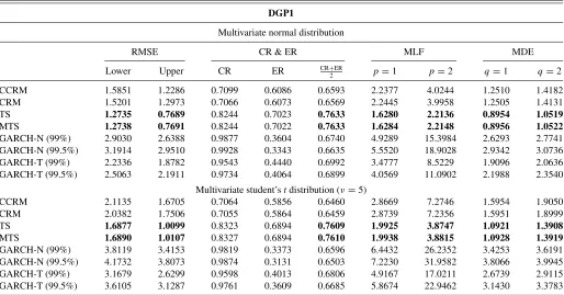
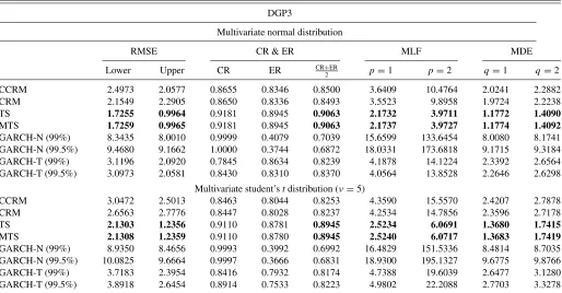
In Tables5and6, we report the values of the four aforemen-tioned evaluation criteria for DGP1 and DGP3, respectively.
Results for DGP2 and DGP4 are available in the the online Appendix. The numbers in boldface correspond to the mini-mum losses when we consider the functions RMSE, MLF, and MDE, and to the maximum rates when we consider the weighted CR/ER rates. In each table, we provide two scenarios: in the up-per panel, the DGP is simulated with multivariate normal errors so that our methods TS and MTS perform under the correct distributional assumption, and in the lower panel, the DGP is simulated with multivariate Student-terrors to assess the per-formance of TS and MTS under density misspecification. These are our findings for the four DGPs considered:
1. Across the four DGPs, TS and MTS exhibit superior perfor-mance over the other methods.
2. Across methods, TS and MTS are superior to CCRM and CRM, and these are far better than the GARCH models. The classical methodology embedded in normal or fat-tail location-scale models is by far the worst performer across all evaluation functions and it is very inefficient on delivering an acceptable fitted interval as the ERs show.
3. With misspecified Student-terrors, the losses across all meth-ods are larger than those under correct error specification, which is expected; nevertheless, TS and MTS provide the smallest loss.
Table 5. Methodology evaluation for DGP1 (HIGH persistence and BINDING observability restriction)
DGP1
Multivariate normal distribution
RMSE CR & ER MLF MDE
Lower Upper CR ER CR+ER
2 p=1 p=2 q=1 q=2
CCRM 1.5851 1.2286 0.7099 0.6086 0.6593 2.2377 4.0244 1.2510 1.4182
CRM 1.5201 1.2973 0.7066 0.6073 0.6569 2.2445 3.9958 1.2505 1.4131
TS 1.2735 0.7689 0.8244 0.7023 0.7633 1.6280 2.2136 0.8954 1.0519
MTS 1.2738 0.7691 0.8244 0.7022 0.7633 1.6284 2.2148 0.8956 1.0522
GARCH-N (99%) 2.9030 2.6388 0.9877 0.3604 0.6740 4.9289 15.3984 2.6293 2.7741
GARCH-N (99.5%) 3.1914 2.9510 0.9928 0.3343 0.6635 5.5520 18.9028 2.9342 3.0736
GARCH-T (99%) 2.2336 1.8782 0.9543 0.4440 0.6992 3.4777 8.5229 1.9096 2.0636
GARCH-T (99.5%) 2.5063 2.1911 0.9734 0.4064 0.6899 4.0569 11.0902 2.1988 2.3540
Multivariate student’stdistribution (ν=5)
CCRM 2.1135 1.6705 0.7064 0.5856 0.6460 2.8669 7.2746 1.5954 1.9050
CRM 2.0382 1.7506 0.7055 0.5864 0.6459 2.8739 7.2356 1.5951 1.8999
TS 1.6877 1.0099 0.8323 0.6894 0.7609 1.9925 3.8747 1.0921 1.3908
MTS 1.6890 1.0107 0.8327 0.6894 0.7610 1.9938 3.8815 1.0928 1.3919
GARCH-N (99%) 3.8119 3.4153 0.9819 0.3373 0.6596 6.4432 26.2352 3.4253 3.6191
GARCH-N (99.5%) 4.1732 3.8073 0.9874 0.3131 0.6503 7.2230 31.9582 3.8066 3.9945
GARCH-T (99%) 3.1679 2.6299 0.9598 0.4013 0.6806 4.9167 17.0211 2.6739 2.9115
GARCH-T (99.5%) 3.6105 3.1287 0.9761 0.3609 0.6685 5.8674 22.9462 3.1430 3.3783
Table 6. Methodology evaluation for DGP3 (HIGH persistence and NONBINDING observability restriction)
DGP3
Multivariate normal distribution
RMSE CR & ER MLF MDE
Lower Upper CR ER CR+ER
2 p=1 p=2 q=1 q=2
CCRM 2.4973 2.0577 0.8655 0.8346 0.8500 3.6409 10.4764 2.0241 2.2882
CRM 2.1549 2.2905 0.8650 0.8336 0.8493 3.5523 9.8958 1.9724 2.2238
TS 1.7255 0.9964 0.9181 0.8945 0.9063 2.1732 3.9711 1.1772 1.4090
MTS 1.7259 0.9965 0.9181 0.8945 0.9063 2.1737 3.9727 1.1774 1.4092
GARCH-N (99%) 8.3435 8.0010 0.9999 0.4079 0.7039 15.6599 133.6454 8.0080 8.1741
GARCH-N (99.5%) 9.4680 9.1662 1.0000 0.3744 0.6872 18.0331 173.6818 9.1715 9.3184
GARCH-T (99%) 3.1196 2.0920 0.7845 0.8634 0.8239 4.1878 14.1224 2.3392 2.6564
GARCH-T (99.5%) 3.0973 2.0581 0.8430 0.8310 0.8370 4.0564 13.8528 2.2646 2.6298
Multivariate student’stdistribution (ν=5)
CCRM 3.0472 2.5013 0.8463 0.8044 0.8253 4.3590 15.5570 2.4207 2.7878
CRM 2.6563 2.7776 0.8447 0.8028 0.8237 4.2534 14.7856 2.3596 2.7178
TS 2.1303 1.2356 0.9110 0.8781 0.8945 2.5234 6.0691 1.3680 1.7415
MTS 2.1308 1.2359 0.9110 0.8780 0.8945 2.5240 6.0717 1.3683 1.7419
GARCH-N (99%) 8.9350 8.4656 0.9993 0.3992 0.6992 16.4829 151.5336 8.4814 8.7035
GARCH-N (99.5%) 10.0825 9.6664 0.9997 0.3666 0.6831 18.9300 195.1327 9.6775 9.8766
GARCH-T (99%) 3.7183 2.3954 0.8416 0.7932 0.8174 4.7388 19.6039 2.6477 3.1280
GARCH-T (99.5%) 3.8918 2.6454 0.8914 0.7533 0.8223 4.9802 22.2088 2.7703 3.3278
4. Across DGPs, DGP1, and DGP3, which have high persis-tence in the conditional mean, have the smallest losses, and in particular, TS and MTS deliver unmatched performance even in the cases of misspecified distributional assumptions. 5. DGP2 and DGP4 have low persistence in the conditional mean. In these two specifications, the coefficients are all very close to zero; thus, in these cases, the constraints imposed by CCRM and CRM are not so restrictive and, as a consequence, the performance of CCRM and CRM is close to that of TS and MTS, but the performance of the location-scale models is still far behind the other methods.
6. Only for DGP4 with low persistence in mean and nonbinding observability restriction, the performance of all methods is roughly equivalent, which is expected as all constraints are relaxed.
In summary, when the researcher faces an interval-valued dataset, a priori, she does not know the persistence of the data and whether the observability restriction is or is not binding; thus, it is advisable to start the estimation of the model by im-plementing TS or/and MTS. If there is high persistence in the conditional mean, even if the observability restriction is non-binding, it pays off to implement TS and MTS as the losses are substantially smaller than those from the competing methodolo-gies. In addition, the implementation of a location-scale model also entails the choice of distributional assumptions, which is subject to misspecification issues.
5.2 In-Sample Evaluation Criteria: Mean Estimates, Bias, and MSE
We compare the mean estimates of the parameters in the conditional mean delivered by TS and MTS with those provided by CCRM and CRM. As before, we consider four DGPs with
correctly specified multivariate normal errors and with Student-t
errors to assess the effect of density misspecification.
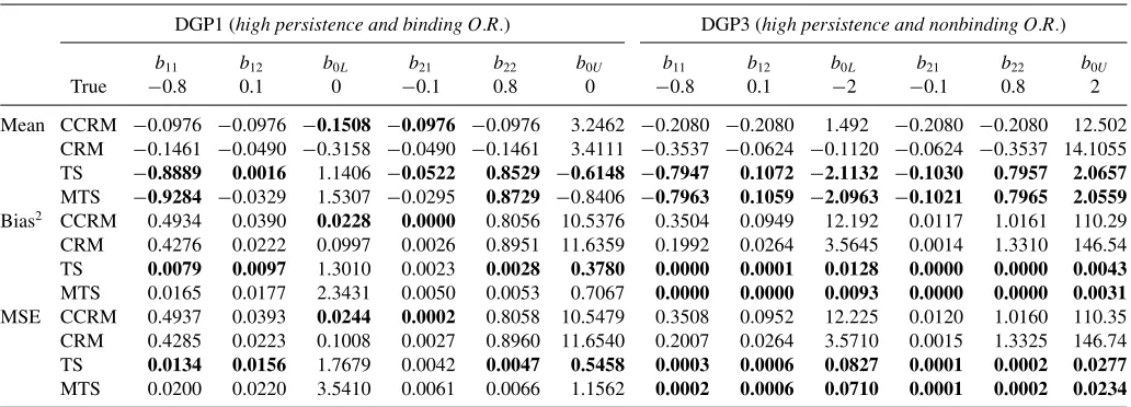
For DGP1 and DGP3, we present the simulation results in Table 7 for the case of multivariate normal errors and in Table 8for multivariate Student-terrors (five degrees of free-dom). Similar tables for DGP2 and DGP4 can be found in the the online Appendix. The numbers in boldface are the best es-timates, the lowest bias and the lowest mean-square error. For normal errors, when the restriction is binding and there is high persistence (DGP1), CCRM and CRM perform very badly. The mean estimates have a large bias and frequently the wrong sign. On the contrary, TS and MTS deliver unbiased estimates with the lowest mean-square error. When the process has low per-sistence (DGP2), the best estimation method is MTS, which delivers unbiased estimates. TS suffers from the multicollinear-ity problem explained earlier and thus it is not recommended if our interest is in understanding the dynamics of the conditional mean. CCRM and CRM estimates are not recommended either because of their large bias. In DGP3 and DGP4, the observ-ability restriction is nonbinding but the results are very similar. When the process has high persistence (DGP3), either TS or MTS deliver unbiased estimates with the lowest mean-square error, and CCRM and CRM generate highly biased estimates. When the process has low persistence (DGP4), MTS is the best performer because it takes care of the multicollinearity problem and delivers unbiased estimates.
For Student-t errors, when the observability restriction is binding and there is high persistence (DGP1), the best per-former is TS followed by MTS as they provide estimates with the lowest biases and capture the right dynamics. On the other hand, CCRM and CRM do not capture the persistence in the conditional mean and their estimates are highly biased. A com-mon problem to these four methods is that the estimates of the constants are very biased. However, in TS and MTS, these
Table 7. Simulation results of DGP1 and GDP3 with multivariate normal errors
DGP1 (high persistence and binding O.R.) DGP3 (high persistence and nonbinding O.R.)
b11 b12 b0L b21 b22 b0U b11 b12 b0L b21 b22 b0U
True −0.8 0.1 0 −0.1 0.8 0 −0.8 0.1 −2 −0.1 0.8 2
Mean CCRM −0.0986 −0.0986 −0.1230 −0.0986 −0.0986 2.7143 −0.2168 −0.2168 1.5698 −0.2168 −0.2168 12.3923 CRM −0.1553 −0.0419 −0.2841 −0.0419 −0.1553 2.8754 −0.3703 −0.0634 −0.0909 −0.0634 −0.3703 14.0530 TS −0.7930 0.1081 −0.0348 −0.1017 0.7977 0.0057 −0.8002 0.1014 −2.0135 −0.0999 0.7990 2.0098 MTS −0.7970 0.1046 −0.0112 −0.1017 0.7975 0.0067 −0.7998 0.1018 −2.0184 −0.1001 0.7988 2.0123 Bias2 CCRM 0.4920 0.0394 0.0151 0.0000 0.8075 7.3676 0.3401 0.1004 12.7436 0.0137 1.0340 107.9996 CRM 0.4156 0.0201 0.0807 0.0034 0.9126 8.2677 0.1847 0.0267 3.6448 0.0013 1.3696 145.2742
TS 0.0000 0.0001 0.0012 0.0000 0.0000 0.0000 0.0000 0.0000 2e-04 0.0000 0.0000 0.0001
MTS 0.0000 0.0000 0.0001 0.0000 0.0000 0.0000 0.0000 0.0000 3e-04 0.0000 0.0000 0.0002
MSE CCRM 0.4922 0.0397 0.0163 0.0002 0.8077 7.3736 0.3404 0.1007 12.7738 0.014 1.0340 108.048 CRM 0.4164 0.0202 0.0813 0.0034 0.9134 8.2792 0.1861 0.0267 3.6501 0.0014 1.3710 145.4484
TS 0.0060 0.0061 0.2076 0.0019 0.0021 0.0686 0.0002 0.0005 0.0538 0.0001 0.0002 0.0186
MTS 0.0013 0.0021 0.0295 0.0004 0.0007 0.0091 0.0002 0.0005 0.0510 0.0001 0.0002 0.0174
biases are somehow compensated by the estimates of the coeffi-cients corresponding to the regressor λt−1 so that the overall
estimation generates good fitted intervals with substantially lower losses than those generated by CCRM and CRM as we have seen inTable 5(lower panel). Thus, the misspecification of the multivariate density does not seem to affect substantially the performance of TS and MTS. When the process has low persistence (DGP2), no method seems to deliver overall unbi-ased estimates, and the problem of the estimation of the constant is severe. Note that the design of low persistence with binding observability restriction (DGP2) represents the worst scenario because, by construction, the intervals are very tight; the specifi-cation of the conditional means deliver very small values around zero, so that the regressorλt−1carries all the weight to estimate
fitted intervals with the right order. Yet, TS delivers the small-est losses. In DGP3 and DGP4, the observability rsmall-estriction is nonbinding. When the process has high persistence (DGP3), TS and MTS are superior performers, and they deliver unbi-ased estimates with the lowest mean-square error. CCRM and CRM produce highly biased estimates. When the process has low persistence (DGP4), MTS is the best performer overall.
In summary, evaluating the estimation performance of the four methods, we reach similar conclusions as those when we evaluate their goodness of fit. Even under misspecification of the multivariate density of the errors, if there is high persistence in the conditional mean, whether the observability restriction is binding or not, TS and MTS are superior estimation tech-niques. If the persistence is low and the observability restriction is nonbinding, we recommend MTS, even with a misspecified density. Only when the persistence is low and the observability restriction is binding, the misspecification of the density may play a role on estimating the right dynamics but yet TS and MTS are not dominated by the competing methods and they offer the advantage of preserving the natural order of an interval.
6. EMPIRICAL ILLUSTRATION: SP500 LOW/HIGH RETURN INTERVAL
We highlight the most important aspects of our methodology with the ITS of the daily low/high returns to the SP500 index. The returns are computed with respect to the closing price of the previous day, that is, rht=(Phigh,t −Pclose,t−1)/Pclose,t−1 and
Table 8. Simulation results of DGP1 and DGP3 with multivariate Student-terrors
DGP1 (high persistence and binding O.R.) DGP3 (high persistence and nonbinding O.R.)
b11 b12 b0L b21 b22 b0U b11 b12 b0L b21 b22 b0U
True −0.8 0.1 0 −0.1 0.8 0 −0.8 0.1 −2 −0.1 0.8 2
Mean CCRM −0.0976 −0.0976 −0.1508 −0.0976 −0.0976 3.2462 −0.2080 −0.2080 1.492 −0.2080 −0.2080 12.502 CRM −0.1461 −0.0490 −0.3158 −0.0490 −0.1461 3.4111 −0.3537 −0.0624 −0.1120 −0.0624 −0.3537 14.1055 TS −0.8889 0.0016 1.1406 −0.0522 0.8529 −0.6148 −0.7947 0.1072 −2.1132 −0.1030 0.7957 2.0657 MTS −0.9284 −0.0329 1.5307 −0.0295 0.8729 −0.8406 −0.7963 0.1059 −2.0963 −0.1021 0.7965 2.0559 Bias2 CCRM 0.4934 0.0390 0.0228 0.0000 0.8056 10.5376 0.3504 0.0949 12.192 0.0117 1.0161 110.29 CRM 0.4276 0.0222 0.0997 0.0026 0.8951 11.6359 0.1992 0.0264 3.5645 0.0014 1.3310 146.54
TS 0.0079 0.0097 1.3010 0.0023 0.0028 0.3780 0.0000 0.0001 0.0128 0.0000 0.0000 0.0043
MTS 0.0165 0.0177 2.3431 0.0050 0.0053 0.7067 0.0000 0.0000 0.0093 0.0000 0.0000 0.0031 MSE CCRM 0.4937 0.0393 0.0244 0.0002 0.8058 10.5479 0.3508 0.0952 12.225 0.0120 1.0160 110.35 CRM 0.4285 0.0223 0.1008 0.0027 0.8960 11.6540 0.2007 0.0264 3.5710 0.0015 1.3325 146.74
TS 0.0134 0.0156 1.7679 0.0042 0.0047 0.5458 0.0003 0.0006 0.0827 0.0001 0.0002 0.0277
MTS 0.0200 0.0220 3.5410 0.0061 0.0066 1.1562 0.0002 0.0006 0.0710 0.0001 0.0002 0.0234