Manajemen | Fakultas Ekonomi Universitas Maritim Raja Ali Haji 073500107000000232

(1)

Full Terms & Conditions of access and use can be found at

http://www.tandfonline.com/action/journalInformation?journalCode=ubes20

Download by: [Universitas Maritim Raja Ali Haji] Date: 12 January 2016, At: 17:42

Journal of Business & Economic Statistics

ISSN: 0735-0015 (Print) 1537-2707 (Online) Journal homepage: http://www.tandfonline.com/loi/ubes20

Forecasting Using Bayesian and

Information-Theoretic Model Averaging

George Kapetanios, Vincent Labhard & Simon Price

To cite this article: George Kapetanios, Vincent Labhard & Simon Price (2008) Forecasting

Using Bayesian and Information-Theoretic Model Averaging, Journal of Business & Economic Statistics, 26:1, 33-41, DOI: 10.1198/073500107000000232

To link to this article: http://dx.doi.org/10.1198/073500107000000232

Published online: 01 Jan 2012.

Submit your article to this journal

Article views: 150

(2)

Forecasting Using Bayesian and

Information-Theoretic Model Averaging:

An Application to U.K. Inflation

George K

APETANIOS

Queen Mary University of London, London E1 4NS, U.K. (g.kapetanios@qmul.ac.uk)

Vincent L

ABHARD

European Central Bank, D-60311 Frankfurt, Germany (vincent.labhard@ecb.int)

Simon P

RICE

Bank of England, London EC2R 8AH, U.K. and City University, London EC1V 0HB, U.K. (simon.price@bankofengland.co.uk)

Model averaging often improves forecast accuracy over individual forecasts. It may also be seen as a means of forecasting in data-rich environments. Bayesian model averaging methods have been widely ad-vocated, but a neglected frequentist approach is to use information-theoretic-based weights. We consider the use of information-theoretic model averaging in forecasting U.K. inflation, with a large dataset, and find that it can be a powerful alternative to Bayesian averaging schemes.

KEY WORDS: Akaike criteria; Data-rich environment; Forecast combining.

1. INTRODUCTION

A key metric of a satisfactory forecast is precision, often de-fined in a root mean squared error sense, and techniques that can deliver this are highly desirable. Model averaging is one such technique that often improves forecast accuracy over individual forecasts.

Another aspect of forecasting is appropriate methodology in data-rich environments, and in recent years there has been increasing interest in forecasting methods that utilize large datasets. There is an awareness that there is a huge quantity of information available in the economic arena which might be valuable for forecasting, but standard econometric techniques are not well suited to extract this in a useful form. This is not an issue of mere academic interest. Svensson (2004) described what central bankers do in practice: “Large amounts of data about the state of the economy and the rest of the world. . . are collected, processed, and analyzed before each major decision.” In an effort to assist in this task, econometricians began assem-bling large macroeconomic datasets and devising ways of fore-casting with them: Stock and Watson (1999) were in the van-guard of this campaign.

One popular methodology is forecast combination, where formation in many forecasting models, typically simple and in-complete, is combined in some manner. Stepping back, fore-cast combination originated not in the large dataset program, but from observations by forecast practitioners that, for what-ever reasons, combining forecasts (initially by simple averag-ing) produced a forecast superior to any element in the com-bined set. This may seem odd, as if it were possible to identify the correctly specified model [and the data generating process (DGP) is unchanging], then it might seem natural so to do, al-though this is less obvious than it may seem. The true DGP may include very many variables that make it infeasible to estimate, and there is a general benefit from parsimony in forecasting. But the weight of evidence dating back to Bates and Granger (1969)

and Newbold and Granger (1974) reveals that combinations of forecasts often outperform individual forecasts. Recent surveys of forecast combination from a frequentist perspective are to be found in Newbold and Harvey (2002) and Clements and Hendry (1998); see also Clements and Hendry (2002). Models may be incomplete, in different ways; they employ different informa-tion sets. Forecasts might be biased, and biases can offset each other. Even if forecasts are unbiased, there will be covariances between forecasts that should be taken into account. Thus, com-bining misspecified models may, and often will, improve the forecast.

An alternative way of looking at this problem is from a Bayesian perspective. Here it is assumed that there is a distri-bution of models, thus delineating the concept of model uncer-tainty quite precisely. The basic problem, that a chosen model is not necessarily the correct one, can then be addressed in a va-riety of ways, one of which is Bayesian model averaging. From this point of view, a chosen model is simply the one with the best posterior odds; but posterior odds can be formed for all models under consideration, thereby suggesting a straightfor-ward way of constructing model weights for forecast combi-nations. This has been used in many recent applications, for example, forecasting U.S. inflation in Wright (2003a).

There is an analogous frequentist information-theoretic ap-proach. In this context, information theory suggests ways of constructing model confidence sets. We use this term in a broader sense than in the related literature of Hansen, Lunde, and Nason (2005) and Kapetanios, Labhard, and Schleicher (2006). Given we have a set of models, we can define relative model likelihood. Model weights within this framework have been suggested by Akaike (1978). Such weights are easy to con-struct using standard information criteria. Our purpose, then, is

(3)

34 Journal of Business & Economic Statistics, January 2008

to consider this way of model averaging as an alternative to Bayesian model averaging.

In this article we develop information-theoretic alternatives to Bayesian model averaging and assess the performance of these techniques by means of a Monte Carlo study. We then compare their performance in forecasting U.K. inflation. For this, we use a U.K. dataset which emulates the dataset in Stock and Watson (2002) (see the App.). Our findings support those of Wright (2003a), who concluded that Bayesian model aver-aging can provide superior forecasts for U.S. inflation, but we find that the frequentist approach also works well and in some cases better in the cases we examine for U.K. data.

2. FORECASTING USING MODEL AVERAGING

2.1 Bayesian Model Averaging

The idea behind forecasting using model averaging reflects the need to account for model uncertainty in carrying out statis-tical analysis. From a Bayesian perspective, model uncertainty is straightforward to handle using posterior model probabili-ties. See, for example, Min and Zellner (1993), Koop and Pot-ter (2003), Draper (1995), and Wright (2003a, b). Briefly, un-der Bayesian model averaging a researcher starts with a set of models that have been singled out as useful representations of the data. We denote this set asM= {Mi}Ni=1whereMiis theith

of theNmodels considered. The focus of interest is some quan-tity of interest for the analysis, denoted by. This could be a parameter, or a forecast, such as inflationhquarters ahead. The output of a Bayesian analysis is a probability distribution for

given the set of models and the observed data at timet. Denote the relevant information set at timetbyDt, and the probability

distribution as Pr(|D,M₎_{. This is given by}

where Pr(|Mi,Dt)denotes the conditional probability

distri-bution ofgiven a modelMiand the dataDt, and Pr(Mi|Dt)

denotes the conditional probability of the modelMibeing the

true model given the data. Implementation requires two quan-tities to be obtained at each point in time: first, Pr(|Mi,Dt),

which is easily obtained from standard model-specific analysis, and second, the weights, Pr(Mi|Dt). The weights are formed as

part of a stochastic process where Pr(Mi|Dt)is obtained from

Pr(Mi|Dt−1), the conditional probability of the model Mi

be-ing true, given the previous period’s data. This requires prior distributions for Pr(Mi|D0)=Pr(Mi)and Pr(θi|Mi,Dt−1)to be specified.

Thus, we need to obtain a number of expressions for (1) to be operational. First, using Bayes’s theorem,

Pr(Mi|Dt)= tribution of the data given the modelMi and the previous

pe-riod’s data, and

Pr(Dt|Mi,Dt−1)=

Pr(Dt|θi,Mi,Dt−1)Pr(θi|Mi,Dt−1)dθi

(3)

is the likelihood of modelMi, where θi are the parameters of

modelMi. Given this, the quantity of interest is

E(|Dt)=

In theory (see, e.g., Madigan and Raftery 1994), whenis a forecast, this sort of averaging provides better average predic-tive ability than single model forecasts.

2.2 Information-Theoretic Model Averaging

In the context of non-Bayesian methods of forecasting, the idea of model averaging (i.e., forecast combination) has a long tradition starting with Bates and Granger (1969). The aim is to use forecasts obtained during some forecast evaluation pe-riod to determine optimal weights from which a forecast can be constructed along the lines of (4). These weights are usu-ally constructed using some regression method and the avail-able forecasts. But a problem arises ifNis large. For example,

N=93 as in Wright (2003a) requires an infeasibly large fore-cast evaluation period.

Although the literature on model averaging inference is dom-inated by work with Bayesian foundations, there has also been some research based on frequentist considerations. Hjort and Claeskens (2003) provided a brief overview in the context of analyzing model averaging estimators from a likelihood per-spective. Most frequentist work focuses on the construction of distributions and confidence intervals for estimators of parame-ters that take into account, in some way, model uncertainty. Examples include Hurvich and Tsai (1990), Draper (1995), Kabaila (1995), Pötscher (1991), Leeband and Pötscher (2000), and Kapetanios (2001). The work of Burnham and Anderson (1998), on which we build, forms a substantial part of the fre-quentist model averaging work available in the literature. But the present article is one of the first to focus on forecasting as opposed to the construction of confidence intervals in the con-text of frequentist model averaging.

Our alternative to Bayesian model averaging is based on the analogue of Pr(Mi|Dt)for frequentist statistics. Such a

weight-ing scheme has been implied in a series of papers by Akaike and others (see, e.g., Akaike 1978, 1979, 1981, 1983; Bozdo-gan 1987) and expounded further by Burnham and Anderson (1998). Akaike’s suggestion derives from the Akaike informa-tion criterion (AIC). AIC is an asymptotically unbiased mea-sure of minus twice the log-likelihood of a given model. It con-tains a term in the number of parameters in the model, which may be viewed as a penalty for overparameterization. Akaike’s original frequentist interpretation relates to the classic mean-variance trade-off, although Akaike (1979) offered a Bayesian interpretation. In finite samples, when we add parameters there is a benefit (lower bias), but also a cost (increased variance). More technically, from an information-theoretic point of view, AIC is an unbiased estimator of the Kullback and Leibler (1951) (KL) distance of a given model, where the KL distance

(4)

is given by

is the entertained model, andθ∗is the probability limit of the parameter vector estimate forg(x|.).I(f,g)is not known. It can

whereθˆ is the estimator of the parameter vectorθ. However, ˆ when comparing different models g and so is an operational model selection criterion. However, although˜I(f,g)andˆI(f,g)

have the same probability limit, the mean of the asymptotic dis-tribution ofT(I˜(f,g)− ˆI(f,g))is not zero. Akaike’s main con-tribution was to derive an expression for this bias under certain regularity conditions. In particular, Akaike showed that the as-ymptotic expectation ofT(˜I(f,g)− ˆI(f,g))isp, wherepis the dimension ofθ. More details on the derivation of this asymp-totic expectation may be found in, for example, Gourieroux and Monfort (1995, pp. 308–309).

So the difference of the AIC for two different models can be given a precise meaning. It is an estimate of the differ-ence between the KL distance for the two models. Further, exp(−1/2i)is the relative likelihood of modeli, wherei=

AICi−minjAICjandAICidenotes the AIC of theith model in

M. Thus, exp(−1/2i)can be thought of as the odds for the

ith model to be the best KL distance model inM_{. So this} quan-tity can be viewed as the weight of evidence for modelito be the KL best model given that there is some model inMthat is KL best as a representation of the available data. Note that we do not require the assumption that the true model belongs to M_{. We are only considering the ranking of models in terms of} KL distance. It is natural to normalize exp(−1/2i)so that

Akaike criterion is only one of several criteria that can form the basis of such weights, we also consider weights based on the Schwarz information criterion (SIC), which has a similar ra-tionale. We consider both versions of the information-theoretic model averaging (ITMA) approach in the exercises we report below: one based on AIC weights (AITMA), and another based on SIC weights (SITMA).

We notewiare not the relative frequencies with which given

models would be picked up according to AIC as the best model givenM_{. Since the likelihood provides a superior measure of} data-based weight of evidence about parameter values com-pared to such relative frequencies (see, e.g., Royall 1997), it is reasonable to suggest that this superiority extends to evidence about a best model given M. In Bayesian language, the wi

might be thought of as model probabilities under

noninforma-tive priors. However, this analogy should not be taken literally as these model weights are firmly based on frequentist ideas and do not make explicit reference to prior probability distributions about either parameters or models.

3. MONTE CARLO EVIDENCE

We now undertake a small Monte Carlo study to explore the properties of various model averaging techniques in the context of forecasting. As we discussed above, model averaging aims to address the problem of model uncertainty in small samples. There are two broad cases that may be considered. The first is when the model that generates the data belongs to the class under consideration. In this case it addresses the issue that the chosen model is not necessarily the true model, and by assign-ing probabilities to various models provides a forecast that is, to some extent, robust to model uncertainty. The second, perhaps more relevant case, is where the true model does not belong to the class of models being considered. Here there is no pos-sibility that the chosen model will capture all the features of the true model. As a result, the motivation for model averaging becomes stronger, because forecasts from different models can inform the overall forecast in different ways. We examine this latter case.

In the experimental design, we adapt the setup proposed in Fernandez, Ley, and Steel (2001) and subsequently used repeat-edly, for example, in Eklund and Karlsson (2005). It therefore offers a standard problem to examine. LetX₌₍_x₁_{, . . . ,}_x_N₎_be aT×N matrix of regressors, wherexi=(xi,1, . . . ,xi,T)′. The

series in the first 2N/3 columns are given by

xi,t=αixi,t−1+ǫi,t, i=1, . . . ,N,t=1, . . . ,T, (6) whereEis aT×N/3 matrix of standard normal variates. This setup allows for some cross-sectional correlation in the predic-tor variables. The true model is given by

yt=2x1,t−x5,t+1.5x7,t+x11,t+.5x13,t+2.5εt, (8)

where εt is iid N(0,1). The numbering of the variables is

prompted partly by the size of the dataset and features of the models investigated in the source references, but this is not a critical feature of the design. The important point is that none of the models considered is the true DGP.

The design in Eklund and Karlsson (2005) setsN=15 and

αi=0. We generalize it in two directions. First, we setN=60,

the nearest round number to our own dataset. Second, we let

αi∼U(.5,1). Theαiintroduce persistence, which we allow to

be random.

The benchmark is the forecast produced by a simpleAR(1)

model foryt. For the remaining forecasts, we use the model

yt+h=a′xt+byt+εt (9)

for the h-step-ahead forecast, wherext is aK-dimensional

re-gressor set, andKtakes the value of 1 or 2. AsKis no greater than 2, the true model can never be selected.

The combinations we evaluate are based on the complete set of models of form (9). The first three combinations are

(5)

duced by Bayesian model averaging (BMA), which in some sense are benchmarks given their wide adoption, differing by a shrinkage parameter described below. The Bayesian weights are set following Wright (2003a). In particular, we set the model prior probabilitiesP(Mi)to the uninformative priors 1/N. The

prior for the regression coefficients is chosen to be given by N(0, φσ2(X′X)−1), conditional onσ2, whereXis theT×p re-gressor matrix for a given model andpis the number of regres-sors. We assume strict exogeneity of theX. The improper prior forσ2is proportional to 1/σ2. The specification for the prior of the regression coefficients implies a degree of shrinkage toward zero (which implies no predictability). The degree of shrink-age is controlled by φ. The rationale is that some degree of shrinkage steers away from models that may fit well in sample (by chance, or because of overfitting) but have little forecasting power. There is empirical evidence that such shrinkage is ben-eficial for out-of-sample forecasting, but no a priori guidance for what values should be selected. Following Wright (2003a), we consider conventional choices of φ=20,2, .5. Given the above, routine integration gives model weights that are propor-tional to

(1+φ)−p/2S−(T+1), (10) where

S2=Y′Y−Y′X(X′X)−1X′Y φ

1+φ (11)

andYis theT×1 regressand vector.

We next consider the ITMA weights introduced previously, namely AITMA and SITMA. Finally, we examine equal-weight model averaging (AV) where the weights are given by 1/N. This last scheme, employed, for example, in Stock and Watson (2004) (see also Stock and Watson 2003), is commonly used and often thought to work well in practice.

We setT=50,100. The forecast evaluation period for each sample is the last 30 observations. We examine the forecast horizons h=1, . . . ,8. For all model averaging techniques we consider two different classes of models over which the weight-ing scheme is applied. The first is all models with one predictor variable (K=1), and the second all models with two predic-tor variables (K=2), neither of which contains the true model. We do not allow for higherKfor two reasons. First, most fore-casting models used in practice, and found to have good per-formance, are parsimonious. Second, weights are assigned to all members of the model class. With our setup andK=2, we have 1,770 models to consider. For (say)K=3 the number of models rises to 34,220 and therefore becomes computationally intensive. Methods to search the model space efficiently do ex-ist that bypass this problem. One is that discussed by Fernan-dez, Ley, and Steel (2001) and based on Markov chain Monte Carlo algorithms. Another is that by Kapetanios (2007) who used genetic and simulated annealing algorithms to search for good models in terms of information criteria. But we do not explore these methods in this article.

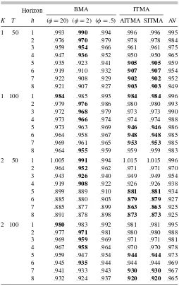
Results for forecast performance in terms of RMSE relative to the benchmark are given in Table 1. The best forecast method in a particular row (i.e., for givenK,T, andh) is indicated in bold. These are evaluated to three decimal places, so in some cases more than one model is “best,” although at higher levels of numerical precision there is always a single best performer. Variations in performance are reasonably large. It is

immedi-Table 1. Monte Carlo study: RMSE of various model averaging schemes

NOTE: BMA indicates Bayesian model averaging whereφindicates shrinkage factor. AITMA, SITMA indicate Akaike, Schwarz information criteria weights. AV indicates sim-ple average.Boldindicates best forecast in row (to third decimal place).

ately evident that for this design the simpleAR(1)benchmark does not perform well, being dominated for most combinations of K,T, and h by the combined forecasts. Simple averaging does better than the AR but is never best. In the Bayesian cases, the low shrinkage parameter tends to do worst. A high shrink-age parameter improves performance, but performance is best for the intermediate value. It is best in 16 out of 32 cases, es-pecially for short horizons. The average value of the RRMSE is .942.

Our main interest is in the information-criteria-based meth-ods. The two methods (AITMA and SITMA) are based on penalty factors that are numerically similar in this experiment, and the results are correspondingly close. As can be seen, they do well, especially at longer horizons, where they tend to dom-inate BMA. Both AITMA and SITMA have the best forecast in 15 out of 32 cases, only one less than for the intermediate BMA; similarly, the average RRMSE is a mere .003 greater at .945. The equivalent performance is a robust result across samples and choice ofK. Essentially, it is hard to choose between the in-termediate BMA and the information-theoretic-based methods.

(6)

In the remainder of the article we see whether these conclusions carry over to the real data.

4. EVIDENCE FROM INFLATION FORECASTS

Our primary focus in this article is practical, and in particular on the practice of inflation forecasting using the model averag-ing schemes examined in the Monte Carlo study. The models we consider are a standard specification, as discussed in Stock and Watson (2004). We modify our Monte Carlo design by us-ing ak1-lag autoregressive process augmented with ak2 distrib-uted lag on a single predictor variable. The number of lags in the pair(k1,k2)(i.e., on the lagged dependent variable and the predictor variable) is chosen as(k,1)wherekis chosen opti-mally for each model, each sample, and each forecast horizon using the Akaike information criterion; we refer to these models asARX(k). Consequently, the lag structure for each predictor-variable model may vary with the horizon. Thus, modeli for forecasting horizonhis given by

πt+h=α+

whereπtis U.K. year-on-year CPI inflation,xitis theith

predic-tor variable at timet, andǫtis the error term, with varianceσ2.

As for the Monte Carlo experiment, the errors will exhibit an

MA(h−1)process. We consider 58 predictor variables, where the data span 1980Q2–2004Q1. We further include the AR fore-cast, making a total of 59 forecasts to combine. Alongside the information-theoretic combinations (based alternatively on AIC and SIC as in the Monte Carlo exercise) we consider Bayesian and equal-weight model averaging. The information-theoretic weights are given by (5). The Bayesian weights are given by the scheme discussed in the Monte Carlo section using (10) and (11).

We use data from the period 1980Q2–1990Q1. We evaluate the forecasts over two post-sample periods: 1990Q2–1997Q1 (pre-MPC) and 1997Q2–2004Q1 (MPC). These are natural dates to choose, as from May 1997 monetary policy was set by the Bank of England’s Monetary Policy Committee under an inflation targeting regime. Here we focus on an evaluation in terms of a RMSE criterion; in the working paper version of this article (Kapetanios, Labhard, and Price 2005), we also evalu-ated the combinations in terms of forecast densities. We con-sider horizons up to three years (i.e.,h=1, . . . ,12).

The forecasts are generated using a recursive forecasting scheme. For example, for the first evaluation period models are estimated up to 1990Q1 and 12 forecasts constructed (i.e., for each period between 1990Q2 and 1993Q1). Then the models are re-estimated over the period 1980Q2–1990Q2 and forecasts constructed for the next 12 periods as before. This is repeated for all the possible forecasts within the evaluation period. From each re-estimation, the estimated log-likelihood is used to con-struct the relevant information criterion which is in turn used to construct the information-theoretic weights, and similarly for the Bayesian weights. We report performance in terms of rela-tive RMSE, compared to the benchmark AR model, as well as two other indicators: the percentage of models of the form (12) that perform worse than a given model averaging scheme in

terms of relative RMSE, and the proportion of periods in which the model averaging scheme has a smaller absolute forecast er-ror than the AR model. The results from these three indicators are ranked similarly so we discuss only those from the first. In the relative RMSE tables we report a Diebold–Mariano (DM) test (Diebold and Mariano 1995) of whether the forecast is sig-nificantly different from the benchmark AR model at the 10% level, indicated with an asterisk.

It is well known that the asymptotic distribution of the DM test statistic under the null hypothesis of equal predictive ability for the two forecasts is not normal when the models used to pro-duce the forecasts are nested. A number of solutions have been proposed for this problem; see Corradi and Swanson (2006) for a survey. We use the parametric bootstrap to obtain the neces-sary critical values. An earlier example of the use of the boot-strap for the Diebold–Mariano test statistic is found in Killian (1999). Our bootstrap design is straightforward. Under the null hypothesis the model generating the data is anAR(p)model. We use the parametric bootstrap to construct bootstrap samples for inflation from the recursively estimatedAR(p)model. These bootstrap series are then combined with the predictor variables, which are kept fixed in the bootstrap sample. Forecasts are recursively produced for all the models and model averaging methods considered in the forecasting exercise, in exactly the same way as the original forecasts. Then DM statistics are pro-duced and stored for every bootstrap replication. These statis-tics form the empirical distribution from which the bootstrap critical values are obtained. We use 199 bootstrap replications.

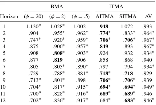
We first consider the MPC forecast evaluation period (Ta-bles 2–4). The Akaike information theory-based AITMA beats the AR benchmark at all horizons. This is also true for the sim-ple average AV, but AITMA provides the best forecast in 8 out of 12 cases whereas the AV provides none. In the table, “best” is defined to three decimal places, so more than one model can be “best.” In several cases the AIC and SIC are numerically iden-tical to three decimal places, but AITMA is absolutely best in all eight cases. The difference from the AR benchmark is sig-nificant in six of the eight cases. This is a strong result, as fore-cast predictive tests have notoriously low power; Ashley (1998)

Table 2. Relative RMSE of out-of-sample CPI forecasts using ARX(k)models (period: 1997Q2–2004Q1)

BMA ITMA

NOTE: *: 10% rejection of Diebold–Mariano test that the forecast differs from the benchmark.Bold_{indicates best forecast in row (to third decimal place). BMA indicates}

Bayesian model averaging whereφindicates shrinkage factor. AITMA, SITMA indicate Akaike, Schwarz information criteria weights. AV indicates simple average.

(7)

Table 3. Proportion of individual models with higher relative RMSE for out-of-sample CPI forecasts usingARX(k)models

(period: 1997Q2–2004Q1)

BMA ITMA

Horizon (φ=20) (φ=2) (φ=.5) AITMA SITMA AV

1 .121 .414 .672 .897 .224 .759 2 .914 .810 .776 .948 .931 .776 3 .931 .897 .845 .948 .948 .845 4 .914 .879 .776 .931 .879 .776 5 .793 .914 .793 .793 .793 .776 6 .862 .931 .845 .862 .862 .793 7 .914 .914 .828 .914 .914 .759 8 .931 .897 .828 .931 .931 .759 9 .983 .914 .810 .983 .983 .776 10 .983 .897 .810 .983 .983 .793 11 .983 .897 .776 .983 .983 .759 12 .983 .897 .776 .983 .983 .776

NOTE: BMA indicates Bayesian model averaging whereφindicates shrinkage factor. AITMA, SITMA indicate Akaike, Schwarz information criteria weights. AV indicates sim-ple average.

concluded that “a model which cannot provide at least a 30% MSE improvement over that of a competing model is not likely to appear significantly better than its competitor over post sam-ple periods of reasonable size.” Moreover, AITMA beats the benchmark by a large margin in many cases—with a RMSE ad-vantage of over 5% in all cases, of 20% or more in eight cases, and more than 30% in three cases. It does particularly well at long horizons, although it is also strong at short horizons. This all makes AITMA a powerful method in this sample and this dataset. The Bayesian BMA scheme works best for intermedi-ateφin terms of the individual best forecast, but highφ(giving the data a high weight) is the best Bayesian scheme overall, al-though clearly inferior to AITMA; and even the low-φscheme is close to dominating the simple averaging scheme AV (which amounts to settingφ=0).

In the working paper version of this article we reported the top-ten ranked models for the Bayesian and

information-Table 4. Proportion of periods in which model has smaller absolute forecast error than AR model for out-of-sample CPI forecasts using

ARX(k)models (period: 1997Q2–2004Q1)

BMA ITMA

1 .375 .406 .438 .500 .313 .500 2 .625 .719 .750 .656 .656 .719 3 .688 .750 .750 .688 .688 .750 4 .625 .656 .594 .750 .688 .594 5 .719 .750 .813 .719 .719 .813 6 .719 .688 .750 .719 .719 .688 7 .719 .750 .719 .719 .719 .781 8 .781 .813 .781 .781 .781 .781 9 .844 .813 .844 .844 .844 .813 10 .875 .875 .906 .875 .875 .844 11 .906 .906 .938 .906 .906 .875 12 .938 .938 .938 .938 .938 .906

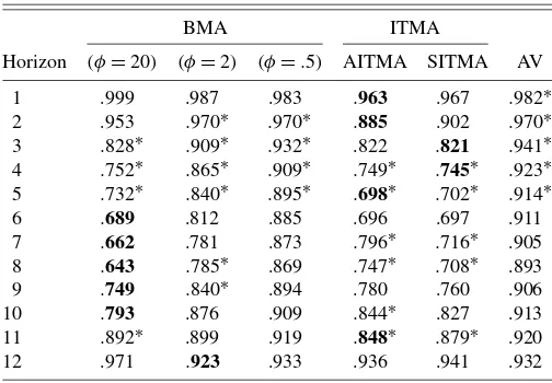
Table 5. Relative RMSE of out-of-sample CPI forecasts using ARX(k)models (period: 1990Q2–1997Q1)

BMA ITMA

1 .999 .987 .983 .963 _.967 _.₉₈₂∗ 2 .953 .970∗ .970∗ .885 _.902 _.₉₇₀∗ 3 .828∗ .909∗ .932∗ .822 .821 _.₉₄₁∗ 4 .752∗ .865∗ .909∗ .749∗ .745∗ _.₉₂₃∗ 5 .732∗ .840∗ .895∗ .698∗ _.₇₀₂∗ _.₉₁₄∗ 6 .689 _.812 _.885 _.696 _.697 _.911 7 .662 _.781 _.873 _.₇₉₆∗ _.₇₁₆∗ _.905 8 .643 _.₇₈₅∗ _.869 _.₇₄₇∗ _.₇₀₈∗ _.893 9 .749 _.₈₄₀∗ _.894 _.780 _.760 _.906 10 .793 _.876 _.909 _.₈₄₄∗ _.827 _.913 11 .892∗ .899 .919 .848∗ _.₈₇₉∗ _.920 12 .971 .923 _.933 _.936 _.941 _.932

NOTE: *: 10% rejection of Diebold–Mariano test that the forecast differs from the benchmark.Boldindicates best forecast in row (to third decimal place). BMA indicates Bayesian model averaging whereφindicates shrinkage factor. AITMA, SITMA indicate Akaike, Schwarz information criteria weights. AV indicates simple average.

theoretic schemes over the same period. The higher isφ, the more weight is put on the variables with the highest in-sample explanatory power. Comparing the high-φ and information-theoretic schemes, the variables selected and weights are very similar. However, the latter two give a little more weight to the best performer, and the subsequent weights decline at a slower rate relative to the Bayesian scheme. The AITMA and SITMA rankings are not identical but are extremely similar. Although there is clearly a concentrated peak on the most important vari-able, in each combination all the models enter with a nonzero weight; in that sense, the information in the entire dataset is be-ing combined, although by the tenth variable the weights in both the SITMA and the BMA with the highestφare down to .5%.

The conclusions remain broadly the same in the pre-MPC forecast evaluation period (Tables 5–7), although the AITMA is no longer so clearly dominant. The best-performing Bayesian (φ=20) combination provides best forecasts at five horizons,

Table 6. Proportion of individual models with higher relative RMSE for out-of-sample CPI forecasts usingARX(k)models

(period: 1990Q2–1997Q1)

BMA ITMA

1 .707 .793 .793 .879 .879 .793 2 .862 .828 .828 .983 .931 .828 3 .931 .862 .828 .948 .948 .810 4 .983 .862 .828 .983 .983 .828 5 .983 .862 .828 .983 .983 .810 6 1.000 .931 .828 .983 .983 .759 7 1.000 .914 .828 .897 .966 .793 8 1.000 .914 .845 .914 .966 .810 9 .966 .914 .845 .948 .948 .845 10 .966 .914 .862 .931 .948 .862 11 .931 .914 .862 .966 .931 .845 12 .759 .897 .879 .879 .862 .879

(8)

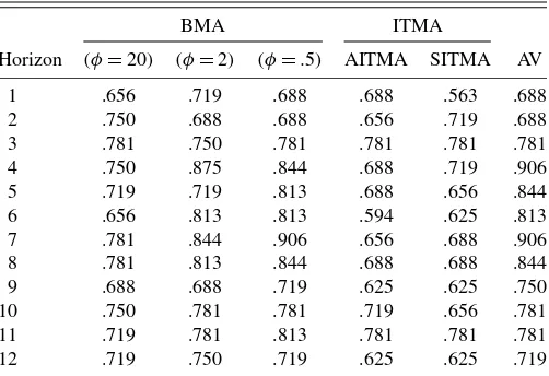
Table 7. Proportion of periods in which model has smaller absolute forecast error than AR model for out-of-sample CPI forecasts using

ARX(k)models (period: 1990Q2–1997Q1)

BMA ITMA

1 .656 .719 .688 .688 .563 .688 2 .750 .688 .688 .656 .719 .688 3 .781 .750 .781 .781 .781 .781 4 .750 .875 .844 .688 .719 .906 5 .719 .719 .813 .688 .656 .844 6 .656 .813 .813 .594 .625 .813 7 .781 .844 .906 .656 .688 .906 8 .781 .813 .844 .688 .688 .844 9 .688 .688 .719 .625 .625 .750 10 .750 .781 .781 .719 .656 .781 11 .719 .781 .813 .781 .781 .781 12 .719 .750 .719 .625 .625 .719

compared to a score of the four best for AITMA. Six of the AITMA forecasts are significantly better than the benchmark, compared to four of the Bayesian. In this period, whereas the AITMA continues to place more weight on fewer variables, the weights are much less concentrated than in the previous case. The variables selected by the high-φBMA and AITMA are now less similar, but there is a high degree of commonality (as there is between the two samples).

Conceptually and practically, the two forecast combina-tion methods are similar; as mencombina-tioned previously, the model weights are not identical but there is a high degree of com-monality. In both cases information is being gleaned from the data in-sample and used to inform the forecast method. In the low-shrinkage case, the frequentist analogy is to the likelihood-weighted scheme. As usual, the information-theoretic measures steer away from the raw likelihood with a parameter penalty, which can be seen as similar to the way information criteria avoid overfitting in standard model selection. It is well known that information criteria can be given a Bayesian interpretation; see the discussion in Kadane and Lazar (2004). There is in prin-ciple no a priori reason to expect a particular approximation to the Bayes factor to perform systematically better or worse than any other; all we can conclude is that in these samples and data the AITMA performs comparably to the Bayesian method. And unlike the Bayesian averaging, there is no requirement to select a particular value for a key parameter (φ). Although we have not explored it in this article, in related work (Kapetanios, Lab-hard, and Price 2006) we have extended the approach to use information-theoretic weights constructed with the predictive likelihood, which is also a good performer. Finally, we note that although we find these information-theoretic techniques work well, and consider them a useful alternative to other techniques, we naturally do not suggest that they would or should be used as the main or only forecasting tool by any central bank.

5. CONCLUSIONS

Model averaging provides a well-established means of im-proving forecast performance which works well in practice and

has sound theoretical foundations. It may also be helpful for another reason. In particular, in recent years there has been a rapid growth of interest in forecasting methods that utilize large datasets, driven partly by the recognition that policy making in-stitutions process large quantities of information, which might be helpful in the construction of forecasts. Standard economet-ric methods are not well suited to this task, but model averaging can help here as well.

In this article we consider two averaging schemes. The first is Bayesian model averaging. This has been used in a variety of forecasting applications with encouraging results. The sec-ond is an information-theoretic scheme that we derive in this article using the concept of relative model likelihood developed by Akaike. Although the information-theoretic approach has re-ceived less attention than Bayesian model averaging, the evi-dence we produce from a Monte Carlo study and an application forecasting U.K. inflation indicate that it has at least some po-tential to produce more precise forecasts and therefore might be a useful complement to other forecasting techniques. There are some advantages in practice. In the frequentist approach the weights are straightforward to compute, and there is less need to make arbitrary assumptions, for example about the shrinkage parameter or the prior distribution.

As there is a clear correspondence with Bayesian averaging, inasmuch as both are based on model performance, it would be odd if the alternative scheme were not also useful. But our work shows that it may outperform Bayesian weights in some cases. Moreover, it has a clear frequentist interpretation and is easy to implement with little judgment required about ancillary assumptions. Whereas it is highly unlikely that a single tech-nique would be more useful than all others in all settings, our work indicates that information-theoretic model averaging may provide a useful addition to the forecasting toolbox.

ACKNOWLEDGMENTS

This article represents the views and analysis of the au-thors and should not be thought to represent those of the Eu-ropean Central Bank, the Bank of England, or Monetary Policy Committee members. We are grateful for comments from two anonymous referees, the editor, and an associate editor.

[Received February 2005. Revised June 2006.]

REFERENCES

Akaike, H. (1978), “A Bayesian Analysis of the Minimum AIC Procedure,”

Annals of the Institute of Statistical Mathematics, 30, 9–14.

(1979), “A Bayesian Extension of the Minimum AIC Procedure of Au-toregressive Model Fitting,”Biometrika, 66, 237–242.

(1981), “Modern Development of Statistical Methods,” inTrends and Progress in System Identification, ed. P. Eykhoff, Paris: Pergamon Press, pp. 169–184.

(1983), “Information Measures and Model Selection,”International Statistical Institute, 44, 277–291.

Ashley, R. (1998), “A New Technique for Postsample Model Selection and Val-idation,”Journal of Economic Dynamics and Control, 22, 647–665. Bates, J. M., and Granger, C. W. J. (1969), “The Combination of Forecasts,”

Operations Research Quarterly, 20, 451–468.

Bozdogan, H. (1987), “Model Selection and Akaike’s Information Criterion (AIC): The General Theory and Its Analytical Extensions,”Psychometrika, 52, 345–370.

(9)

Burnham, K. P., and Anderson, D. R. (1998),Model Selection and Inference, Berlin: Springer-Verlag.

Clements, M. P., and Hendry, D. F. (1998),Forecasting Economic Time Series, Cambridge, U.K.: Cambridge University Press.

(2002), “Pooling of Forecasts,”Econometrics Journal, 5, 1–26. Corradi, V., and Swanson, N. R. (2006), “Predictive Density Evaluation,” in

Handbook of Economic Forecasting, eds. C. W. J. G. G. Elliot and A. Tim-merman, Amsterdam: Elsevier, pp. 197–284.

Diebold, F. X., and Mariano, R. S. (1995), “Comparing Predictive Accuracy,”

Journal of Business & Economic Statistics, 13, 253–263.

Draper, D. (1995), “Assessment and Propagation of Model Uncertainty,” Jour-nal of the Royal Statistical Society, Ser. B, 57, 45–97.

Eklund, J., and Karlsson, S. (2005), “Forecast Combination and Model Aver-aging Using Predictive Measures,” Working Paper 5268, CEPR.

Fernandez, C., Ley, E., and Steel, M. F. (2001), “Benchmark Priors for Bayesian Model Averaging,”Journal of Econometrics, 100, 381–427.

Gourieroux, C., and Monfort, A. (1995),Statistics and Econometric Models, Vol. 2, Cambridge, U.K.: Cambridge University Press.

Hansen, P. R., Lunde, A., and Nason, J. M. (2005), “Model Confidence Sets for Forecasting Models,” Working Paper 2005–2007, Federal Reserve Bank of Atlanta.

Hjort, N. L., and Claeskens, G. (2003), “Frequentist Model Average Estima-tors,”Journal of the American Statistical Association, 98, 879–899. Hurvich, C. M., and Tsai, C.-L. (1990), “The Impact of Model Selection on

Inference in Linear Regression,”American Statistician, 44, 214–217. Kabaila, P. (1995), “The Effect of Model Selection on Confidence Regions and

Prediction Regions,”Econometric Theory, 11, 537–549.

Kadane, J. B., and Lazar, N. (2004), “Methods and Criteria for Model Selec-tion,”Journal of the American Statistical Association, 99, 279–290. Kapetanios, G. (2001), “Incorporating Lag Order Selection Uncertainty in

Pa-rameter Inference for AR Models,”Economics Letters, 72, 137–144. (2007), “Variable Selection Using Non-Standard Optimisation of In-formation Criteria,”Computational Statistics and Data Analysis, to appear. Kapetanios, G., Labhard, V., and Price, S. (2005), “Forecasting Using Bayesian

and Information Theoretic Model Averaging: An Application to U.K. Infla-tion,” Working Paper 268, Bank of England.

(2006), “Forecasting Using Predictive Likelihood Model Averaging,”

Economics Letters, 91, 373–379.

Kapetanios, G., Labhard, V., and Schleicher, C. (2006), “Conditional Model Confidence Sets With an Application to Forecasting Models,” manuscript, Bank of England.

Killian, L. (1999), “Exchange Rates and Monetary Fundamentals: What Do We Learn From Long-Horizon Regressions?”Journal of Applied Econometrics, 14, 491.

Koop, G., and Potter, S. (2003), “Forecasting in Large Macroeconomic Panels Using Bayesian Model Averaging,” Report 163, Federal Reserve Bank of New York.

Kullback, S., and Leibler, R. A. (1951), “On Information and Sufficiency,”The Annals of Mathematical Statistics, 22, 79–86.

Leeband, H., and Pötscher, B. M. (2000), “The Finite-Sample Distribution of Post-Model-Selection Estimators, and Uniform versus Non-Uniform Ap-proximations,” Technical Report TR 2000-03, Institut für Statistik und Deci-sion Support Systems, Universität Wien.

Madigan, D., and Raftery, A. E. (1994), “Model Selection and Accounting for Model Uncertainty in Graphical Models Using Occam’s Window,”Journal of the American Statistical Association, 89, 535–546.

Min, C., and Zellner, A. (1993), “Bayesian and Non-Bayesian Methods for Combining Models and Forecasts With Applications to Forecasting Inter-national Growth Rates,”Journal of Econometrics, 56, 89–118.

Newbold, P., and Granger, C. W. J. (1974), “Experience With Forecasting Uni-variate Time Series and the Combination of Forecasts,”Journal of the Royal Statistical Society, Ser. A, 137, 131–165.

Newbold, P., and Harvey, D. I. (2002), “Forecast Combination and Encompass-ing,” inA Companion to Economic Forecasting, eds. M. Clements and D. F. Hendry, Oxford: Basil Blackwell, Chap. 12.

Pötscher, B. M. (1991), “Effects of Model Selection on Inference,”Econometric Theory, 7, 163–185.

Royall, R. M. (1997),Statistical Evidence: A Likelihood Paradigm, New York: Chapman and Hall.

Stock, J. H., and Watson, M. W. (1999), “Forecasting Inflation,”Journal of Monetary Economics, 44, 293–335.

(2002), “Macroeconomic Forecasting Using Diffusion Indices,” Jour-nal of Business & Economic Statistics, 20, 147–162.

(2003), “Forecasting Output and Inflation: The Role of Asset Prices,”

Journal of Economic Literature, 41, 788–829.

(2004), “Combination Forecasts of Output Growth in a Seven Country Dataset,”Journal of Forecasting, 23, 405–430.

Svensson, L. E. O. (2004), “Monetary Policy With Judgment: Forecast Target-ing,” unpublished manuscript.

Wright, J. H. (2003a), “Bayesian Model Averaging and Exchange Rate Fore-casts,” International Finance Discussion Papers 779, Board of Governors of the Federal Reserve System.

(2003b), “Forecasting US Inflation by Bayesian Model Averaging,” In-ternational Finance Discussion Papers 780, Board of Governors of the Fed-eral Reserve System.

DATA APPENDIX

In this appendix we provide a list of the series used in Sec-tion 4 to forecast U.K. inflaSec-tion. These series come from a dataset that has been constructed to match the set used by Stock and Watson (2002). In total, this dataset has 131 series, com-prising 20 output series, 25 labor market series, 9 retail and trade series, 6 consumption series, 6 series on housing starts, 12 series on inventories and sales, 8 series on orders, 7 stock price series, 5 exchange rate series, 7 interest rate series and 6 mon-etary aggregates, 19 price indices, and an economic sentiment index. We retained the 58 series with at least 90 observations. The series are grouped under 10 categories. For each series we give a brief description: more details, summary statistics, and the transformations applied to ensure stationarity are available on request.

Series 1 to 8: Real output and income:

•S1: Gross domestic product •S2: Manufacturing

•S3: Durable manufacturing •S4: Semidurable manufacturing •S5: Nondurable manufacturing •S6: Mining and quarrying

•S7: Electricity, gas, and water supply •S8: Real households disposable income

Series 9 to 21: Employment and hours:

•S9: UK workforce jobs •S10: Employed, nonagricultural •S11: Employment rate

•S12: Employees total nonagricultural •S13: Employees private nonagricultural •S14: Employee jobs: production •S15: Employee jobs: construction •S16: Employee jobs: manufacturing

•S17: Employee jobs: wholesale and retail trade •S18: Employee jobs: banking, finance, and insurance •S19: Employee jobs: total services

•S20: Employee jobs: public admin. and defense •S21: Average weekly manufacturing hours

Series 22 to 23: Trade:

•S22: BOT: goods •S23: BOT: manufactures

Series 24 to 29: Consumption:

•S24: Household final consumption expenditure •S25: Durable goods

•S26: Semidurable goods •S27: Nondurable goods •S28: Services

•S29: Purchase of vehicles

(10)

Series 30 to 35: Real inventories and inventories sales:

•S30: Change in inventories: manufacturing •S31: Change in inventories: textiles and leather •S32: Manuf and trade invent: nondurable goods •S33: Change in inventories: wholesale

•S34: Change in inventories: retail •S35: Inventory/output mfg and trade

Series 36 to 38: Stock prices:

•S36: FTSE All Share Price Index •S37: FTSE100

•S38: FTSE All Share Dividend Yield

Series 39 to 43: Exchange rates:

•S39: Sterling effective rate •S40: Euro/£

•S41: Swiss Franc/£ •S42: Yen/£ •S43: US$/£

Series 44 to 47: Interest rates:

•S44: Spread 6 months to 1 month •S45: Spread 1 year to 1 month •S46: Spread 5 years to 1 month •S47: Spread 10 years to 1 month

Series 48 to 50: Monetary and quantity credit aggregates:

•S48: M4 •S49: M0

•S50: Reserves and other accounts outstanding