ISSN1842-6298 (electronic), 1843 - 7265 (print) Volume3(2008), 123 – 165
50 YEARS SETS WITH POSITIVE REACH
A SURVEY
-Christoph Th¨ale
Abstract. The purpose of this paper is to summarize results on various aspects of sets with positive reach, which are up to now not available in such a compact form. After recalling briefly the results before 1959, sets with positive reach and their associated curvature measures are introduced. We develop an integral and current representation of these curvature measures and show how the current representation helps to prove integralgeometric formulas, such as the principal kinematic formula. Also random sets with positive reach and random mosaics (or the more general random cell-complexes) with general cell shape are considered.
1
Introduction
This paper is a collection of various aspects of sets with positive reach, which were introduced by Federer in 1959 [4]. Thus, the paper is also a celebration of their 50-th birthday in 2009.
After the developments of integral geometry for convex sets as well as for smooth manifolds in differential geometry, the situation around 1950 was the following: There were two tube formulas (Steiner’s formula and Weyl’s formula), which say that the volume of a sufficiently small r-parallel neighborhood of a convex set or a C2 -smooth submanifoldXinRdis a polynomial inrof degreed, the coefficients of which are (up to some constant) geometric invariants of the underlying set. Unfortunately the the assumptions of both results are quite different, such that each case does not contain or imply the other one. This problem was solved by Federer in this famous paper [4], where he introduced sets with positive reach and their associated curvatures and curvature measures. He was also able tho show a certain tube formula for this class of sets. A comparison with the former cases from convex and differential geometry shows that in this special cases the new invariants coincide with the known ones. Thus, sets with positive reach generalize the notion of convex sets on the one
2000 Mathematics Subject Classification:49Q15; 28A75; 53C65; 60G55; 60D05; 60G57; 52A39. Keywords: Sets with Positive Reach; Curvature Measure; Integral Geometry; Kinematic For-mula; Random Set; Random Mosaic; Current; Normal Cycle; Random Cell Complex.
hand side and the notion of a smooth submanifold on the other. It was also Federer, who proved the fundamental integralgeometric relationship for sets with positive reach, the principal kinematic formula.
With the development of geometric measure theory and especially the calculus of currents, the idea of the so-called normal cycle of a set with positive reach came into play in the early 1980th. This idea paved the wary for explicit representations of Federer’s curvature measures as well as for a simple approach to integral geometry, because many of these problems could be reduced to an application of the famous Coarea Formula. Also extensions to other classes of sets are possible by following this way.
After having developed a solid theory for deterministic sets with positive reach, several well known models from stochastic geometry were lifted up to the case of random sets with positive reach. This includes the theory of random processes of sets with positive reach and their associated union sets. This in particular allows to treat random cell complexes and random mosaics with general cell shape. The main integralgeometric relationships were extended to this random setting, which leads to stochastic versions of the principal kinematic formula and Crofton’s formula. In this paper we like to sketch these developments from the last 50 years. Of course, the material is a selection, which relies more or less on the authors taste. We also do not qualify for completeness. Since proofs are sketched mostly, we try to give de-tailed references trough the existing literature. We like to point out that there is up to now a lack of a comprehensive monograph on this very interesting and beautiful topic. We remark that we will restrict in this paper ourself to the case of curvature measures defined onRd, even if there is also a theory dealing with directional cur-vature measures onRd×Sd−1.
The paper is organized as follows: Section2recalls the situation before 1959. In2.1
important notions and notations from convex geometry are introduced. Section 3
deals with basic properties of sets with positive reach (Section3.1) and the most im-portant tools, associated curvature measures and unit normal cycles (Section3.2). In Section3.3the notion of the normal cycle and the curvature measures are extended to the case of locally finite unions of sets with positive reach. Characterization theorems of these curvature measures using tools from geometric measure theory are explained in 3.4. The topic of Section 4 is integral geometry. First we prove a translative integral formula for sets of positive reach (Section 4.1), which leads to the principal kinematic formula in Section4.2. Here the power of the concept of the unit normal cycle is demonstrated in interplay with the Coarea Formula. In Section
4.3 we extend the theory again to locally finite unions of sets with positive reach. The results are applied in Section5, where integralgeometric formulas from Section
2
Results before 1959
Before 1959 there were two main branches in mathematics dealing with curvature and curvature measures. This are convex geometry and differential geometry. The most important results in these fields will be summarized below. This background provides a solid basis for the understanding and motivation for Federer’s sets with positive reach.
2.1 Convex Geometry
We fix a convex set X ⊆ Rd. For r > 0 its r-parallel set or neighborhood Xr is the set of all points x ∈ Rd with distance to X at most r, i.e. Xr := {x ∈ Rd : dist(X, x)≤r}. If we denote byA⊕B ={a+b:a∈A, b∈B}the Minkowski sum of two setsAandB, the setXr can be interpreted asXr=X⊕B(r), whereB(r) is
a ball with radius r. A fundamental result in convex geometry is Steiner’s formula:
Theorem 1. For a convex body X ⊂ Rd (this is a compact convex set with
non-empty interior) and r > 0, the volume vol(Xr) = Hd(Xr) is a polynomial in r, i.e.
vol(Xr) =Hd(Xr) = d
X
i=0
ωiVd−i(X)ri,
where Vj(X) are coefficients with only depend on X, ωj is the volume of the j -dimensional unit ball andHk denotes thek-dimensional Hausdorff measure (see [5, 2.10.2]).
The proof of this formula is quite easy if one knows that any convex body X can be approximated by a sequence (Pn) of polyhedra. Now one observes that the
formula is true for polyhedra and transfers the result via the above approximation to arbitrary convex bodies. For more details see for example the monograph [25]. The numbersV0(X), . . . , Vd(X) are usually called intrinsic volumes ofX. In
partic-ular we have for any convex bodyX ⊂Rd 1. V0(X) = 1,
2. V1(X) = 2ωdωd−d1b(X), where b(K) is the mean breadth ofX (cf. [25]),
3. Vd−1(X) = 12Hd−1(∂X), where ∂X is the boundary of the set X,
4. Vd(X) =vol(X) =Hd(X).
In the literature there is also another normalization used. We call
Wi(X) := ωni i
the i-th Quermassintegral of X. The name comes from the following projection formula, which is often used as a definition: Let X be a convex body inRd and for i∈ {1, . . . , d−1},L(d, i) the family ofi-dimensional linear subspaces ofRdequipped with the unique probability measure dLi. We denote for L ∈ L(d, i) byπL(X) the
orthogonal projection ofX onto L, which is again a convex set. Then we have Vi(X) =
d i
ωd
ωiωd−i
Z
L(d,j)
Vj(πL(K))dLi(L).
Here, the integrandVj(πL(X)) is the volume of the projection of X ontoL. Hence,
we can call it Quermass of X in directionL⊥.
The functionals Vi : K → R, where K is the family of convex bodies, have the
following important properties: They are
(i) motion invariant, i.e. Vi(gX) =Vi(X) for any euclidean motiong,
(ii) additive, i.e. Vi(X∪Y) =Vi(X) +Vi(Y)−Vi(K∩Y) for allX, Y, X∪Y ∈ K,
(iii) continuous, i.e. ifXn→X in Hausdorff metric thenVi(Xn)→Vi(X),
(iv) homogeneous, i.e. Vi(λX) =λiVi(X) for allλ >0,
(v) monotone, i.e. X⊆Y implies Vi(X)≤Vi(Y),
(vi) non-negative, i.e. Vi(X)≥0 for allX ∈ K.
We will see now that properties (i)-(iii) are sufficient to characterize the intrinsic volumes. This is the content of Hadwiger’s Theorem:
Theorem 2. Let Ψ :K →R a functional which is motion invariant, additive and continuous. ThenΨcan be written as a linear combination of the intrinsic volumes, i.e. there are real constants c0, . . . , cd, such that
Ψ =
d
X
i=0
ciVi.
The proof of this theorem uses deep methods of discrete geometry, see [10]. A short proof was given by Klain [11]. The so-called principal kinematic formula is now an easy consequence of Hadwiger’s Theorem:
Corollary 3. Let X, Y ∈ K and i∈ {0, . . . , d}. Then
Z
SO(d)⋉Rd
Vi(X∩gY)dg=
X
m+n=d+i
γ(m, n, d)Vm(X)Vn(Y),
Remark 4. The measuredg is the product measure with factorsdHdanddϑ, where
dϑ is a Haar measure on the group SO(d). Here and for the rest of this paper we will use the following normalization of dϑ:
ϑ{g∈SO(d) :gO ∈M}=Hd(M),
where O is the origin and M some subset ofRd. With this normalization in mind
it is clear that dϑ is not a probability measure on SO(d).
For the proof one has to observe that for fixedXthe left hand side is a functional in the sense of Theorem2. Now, fixingY instead ofXwe have the same situation and can apply Hadwiger’s Theorem once again. It remains to shown that the constant equals γ(m, n, d). This can be done, by plugging balls with varying radii into the formula.
An obvious consequence is the so-called Crofton formula:
Corollary 5. ForX ∈ K, k∈ {0, . . . , d} and i∈ {0, . . . , k} we have
Z
E(d,k)
Vi(X∩E)dE=γ(i, k, d)Vd+i−k(X),
whereE(d, k)is the space ofk-dimensional affine subspaces ofRd with Haar measure
dE.
We remark here that it is possible to localize all these formulas in the language of curvature measures. We omit the details in the convex case, since curvature measures will be considered in detail below for sets with positive reach, which includes the case of convex sets. For more details we refer to [25]. We also like to remark that it is possible to extend the intrinsic volumes as well as the curvature measures to the so-called convex ring R. This is the family of locally finite unions of convex sets. For details we also refer to [25], because we will work out in Section 3.3 in detail such an extension in the case of locally finite unions of sets with positive reach and the convex ringR is included in these considerations.
We like to finish this section with an introduction to translative integral geometry for convex sets (see for example [9] for more details). As a main tool we introduce the so-called mixed volumes:
Theorem 6. Let X1, . . . , Xm ∈ K, m ∈ N and λ1, . . . , λm ≥0. Then there exists a representation of the volume of the linear combination λ1X1⊕. . .⊕λmXm of the following form:
vol(λ1X1⊕. . .⊕λmXm)) m
X
k1,...,kd=1
λk1· · ·λkdVk1...kd,
We write V1...d=V(X1, . . . , Xd) and called it mixed volume ofX1, . . . , Xd. The
mixed volumes have the following important properties:
1. V(X1, . . . , Xd) is symmetric, i.e.
V(X1, . . . , Xm, . . . , Xn, . . . , Xd) =V(X1, . . . , Xn, . . . , Xm, . . . , Xd)
for all 1≤n < m≤d,
2. V(X1, . . . , Xd)≥0 and V is monotone in each component,
3. V is translation invariant in each component and V(ϑX1, . . . , ϑXd) =V(X1, . . . , Xd)
for all ϑ∈SO(d),
4. V is continuous onKd wrt. the natural product topology,
5. we have for x∈ K and r >0
A comparison of the last point and Steiner’s formula especially shows
Vd−i(X) =
Tis concept can also be localized, which leads to mixed curvature measures. They will be introduced below for sets with positive reach.
Translative integral geometry for convex sets deals with integrands of the formVi(X∩
τz(Y)), whereτz(A),z∈Rd, denotes the translation of a setA by a vectorz. As a
main result we state the following principal translative integral formula for convex bodies, where i= 0:
Theorem 7. For two convex bodiesX and X we have
Z
the summands do not have in general a simple explicit interpretation. In section4.1
2.2 Differential Geometry
We consider ad-dimensional submanifoldMdinRdwithC2-smooth boundary∂Md
and denote by ν(x) the unique unit outer normal vector of Md at x ∈ ∂Md. The
mapν :∂Md→ Sd−1 is called Gauss map. Since ∂Md is C2-smooth we know that
the differential
Dν(x) :Tx∂Md→Tν(x)Sd−1 ≡Tx∂Md
exists in all points x ∈ ∂Md. We assume that in a neighborhood of x ∈ ∂Md the
surface is parameterized by F :U →Rd. Then L=−Dν◦(DF)−1
is a well defined symmetric endomorphism on Tx∂Md. Hence, there exist
eigenval-uesk1(x), ..., kd−1(x) (called principal curvatures) and eigenvectorsa1(x), ..., ad−1(x)
(usually called principal directions).
Definition 8. The elementary symmetric functions σk of order k= 0, ..., d−1 are defined as
σk(k1(x), ..., kd−1(x)) =
X
1≤i1<...<ik≤d−1
ki1(x)· · ·kik(x).
They are used in the following
Definition 9. The k-th integral of mean curvature (also called Lipschitz-Killing curvature) of Md is defined as
Ck(Md) :=Od−−11−k
Z
∂Md
σd−1−k(k1(x), ..., kd−1(x))dHd−1(x), k= 0, . . . , d−1 whereOm is the surface area of them-dimensional unit ball. Define furtherCd(Md) := Hd(Md).
In particular we have in the case, where X is compact 1. C0(Md) =χ(Md) (Gauss-Bonnet Theorem),
2. Cd−1(Md) = 12Hd−1(∂Md),
3. Cd(Md) =Hd(Md) =vol(Md).
One of the fundamental theorems in differential geometry is Wely’s Tube For-mula, which has its origin in a statistical problem [28]:
Theorem 10.
Hd((Md)ε) = d
X
k=0
ωkCd−k(Md)εk,
where the ε-parallel set(Md)ε of Md is defined as(Md)ε:={x∈Rd:dist(x, Md)≤
Integral geometry for smooth hypersurfaces and m-surfaces (m < d−1) in Rd was developed in [26, Ch. V] and we refer to this monograph for further details. We only like to mention here, that similar formulas as in Corollary 3 and Corollary 5
are true in this case. But up to a constant, thek-th intrinsic volume is replaced by thek-th integral of mean curvature, k= 0, . . . , d. This is the reason, why we omit to state them here explicitly. Furthermore, the integralgeometric results below will cover the case of C2-smooth submanifolds.
3
Sets with Positive Reach
We introduce in this section the class of sets with positive reach and their geometric properties. The focus of our considerations lies on curvature measures for this class of sets. Therefore, the so-called unit normal cycle is used as a fundamental toll in singular curvature theory. It also helps to extend the curvature measures to the class of locally finite unions of sets with positive reach.
3.1 Definition and Basic Properties
Sets with positive reach are characterized by their unique foot point property in a positive r-parallel set. This property ensures that suitable small parallel neighbor-hoods have no self-intersections and this allows to compute their volume. This will lead to a Steiner-type formula and a definition of curvature measures for sets with positive reach, which extends the cases treated in Section 2.
Definition 11. The reach of a set X ⊆Rd is defined as
reach X:= sup{r≥0 :∀y∈Xr ∃!!x∈X nearest to y}.
We say that a setX has positive reach, if reachX >0 and denote byP R the family of sets with positive reach.
We can also formulate this property as follows: A set X has positive reach, if one can roll up a ball of radius at most reach X > 0 on the boundary ∂X. Note that sets with positive reach are necessarily closed subsets ofRd. This will be useful when we deal with random sets with positive reach in Section5, since there exists a well developed theory of random closed sets inRd, see for example [12].
Remark 12. It is also possible to define the class of sets with positive reach on smooth and connected Riemannian manifolds. By a Theorem of Bangert [1, p. 57] this property does not depend on the Riemannian structure of the underlying man-ifold. Hence, the theory of sets with positive reach in Rd (and also their additive
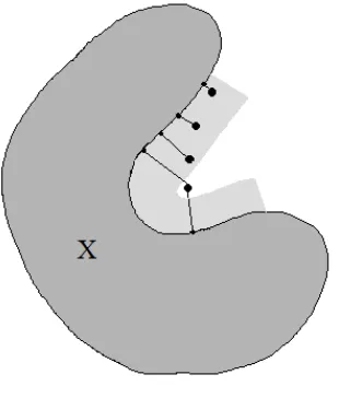
Figure 1: A non-convex setXwith positive reach: 4 points inR2 and its foot points on X, the lower one is not unique
We will now show that the classes of sets introduced in Section 2 are included in our discussion:
Proposition 13. A set X is convex if and only if reach X= +∞.
One direction is clear, the other corresponds to [25, Thm. 1.2.4]. It is a well known fact in differential geometry that the exponential map of a closed C2
-submanifold is a bijection in a suitable small neighborhood of the -submanifold. But this leads immediately to
Proposition 14. Compact C2-smooth submanifolds X of Rd have positive reach.
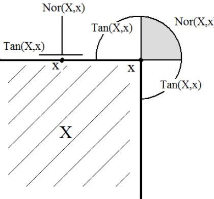
The closed convex cone of tangent vectors of X ∈ P R atx will be denoted by Tan(X, x). Here, a vector u∈Sd−1 belongs to Tan(X, x) if there exists a sequence
(xn)⊂X\ {x}, such that |xxnn−−xx| converges to u. The normal cone of X atx
Nor(X, x) ={u∈Sd−1 :hv, ui ≤0, v∈Tan(X, x)}
is the dual cone of Tan(X, x). For an illustration of these concepts see Figure 2. The set
norX:={(x, u)∈Rd×Sd−1:x∈X, u∈nor(X, x)}
Figure 2: A set X and two points x∈X with associated tangent and normal cone
Remark 15. The unit normal bundle is a (d−1)-dimensional rectifiable set in
Rd×Sd−1 ⊆ R2d in the sense of Federer [5, 3.2.14]. This means that nor X is
Hd−1-measurable and there exist Lipschitz functions f
1, f2, . . . : Rd−1 → R2d and bounded setsE1, E2, . . .⊂Rd−1 such that
Hd−1 nor X\
∞
[
i=1
fi(Ei)
!
= 0.
We recall here the following result, which was proved by Federer [4]. It relates the boundary of a set X∈P R with its unit normal bundle:
Proposition 16. Assume 0< r≤ε < R=reach X. Then (1) ϕ:∂Xr →nor X:y7→
ΠX(y),y−ΠX(y)
r
is bijective and bi-Lipschitz.
(2) f :nor X×(0, ε]→(Xε\X) : (x, u, r)7→x+ru is bijective and bi-Lipschitz. Here ΠX :Rd→X is the metric projection ontoX, i.e. ΠX(x) is the set of nearest points of X tox∈Rd.
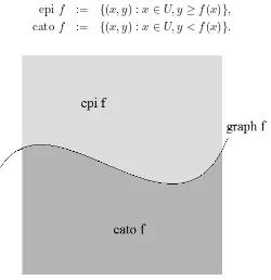
Sets with positive reach are closely connected with Lipschitz functions and semicon-cave functions. Federer has shown in [4, 4.20] that a Lipschitz functionf :Rm →Rn has Lipschitz derivative if and only if the graph off has positive reach. This illus-trates very well of what it means for a submanifold to have positive reach. For a functionf :Rm → R, U ⊂Rm open, we define its epigraph and its catograph (see Figure3) as
epif := {(x, y) :x∈U, y ≥f(x)}, catof := {(x, y) :x∈U, y < f(x)}.
Figure 3: The graph of a functionf(x) with its epi- and catograph
We say that f is semiconcave, if for each bounded open set V ⊂ U with closure(V)⊆U there exists a constantC <∞, such that the restriction of g(x) := Ckx2k2−f(x) to the setV is a convex function. We definesc(f, V) to be the smallest such constant C,sc(f, U) := sup
V
sc(f, V) and sc0(f, U) := max{sc(f, U),0}. Then
Fu [6, Th. 2.3] has proved
Proposition 17. For a locally Lipschitz function f :Rm →R we have sc0(f,Rm)≥reach(cato f)−1.
For the opposite direction of the inequality we have [6, Cor. 2.8]
Proposition 18. Let U ⊂ Rm be open and convex, f : U → R Lipschitz with
exists a pointp∈Rm+1 for which B(p, r)∩cato f ={a, f(a)}, where B(p, r) is the
closed ball around p with radiusr. Then
reach(cato f)−1 ≥(1 +L2)−3/2sc(f, U).
Summarizing these results we get under the conditions of Proposition18
sc0(f, U)−1 ≤reach(cato f)≤(1 +L2)3/2sc(f, U)−1.
From a version of the implicit function theorem for Lipschitz functions, which says that if p∈U ⊂Rm is a regular value (this is 0 does not belong to the subgradient at p) and f : U → R is semiconcave then there exists V ⊂ U, p ∈ V, a rotation ϑ∈SO(m), an open set W ⊂Rm−1 and a semiconcave function g :W →R, such that ϑ(f−1(f(p)∩V)) = graph g and f−1([f(p),∞)) is locally the catograph of g, we obtain [6, Cor. 3.4], which is also a special case of a result in [1]:
Theorem 19. Suppose that f :Rm →Ris semiconcave and proper (this is that the
pre-image of a compact set is compact). Let t be a regular value of f. Then reach(f−1([f(t),∞)))>0.
An immediate consequence of the last Theorem is
Corollary 20. Let S ⊂ Rd be a compact set. Denote by distS(x) := inf{kx−sk : s∈S} the distance function of S, bycrit(distS) the set of critical points ofdistS (a point is critical if it is not regular) and byC :=distS(crit(distS)) the set of critical values. Then forr ∈(0,∞)\C, the set closure(Rd\Sr) has positive reach.
Moreover one can show thatH(d−1)/2(C) = 0. This in particular implies that for
d= 2, closure(Rd\Sr) has positive reach for all r >0. Ford= 3 this is only true for almost allr.
Corollary20 has various applications. For example one can show that closure(Rd\ Xr) has positive reach if X∈ R orX ∈UP R (for a definition see Section3.3). This
property is also fulfilled for certain Lipschitz manifolds (cf. [22]) or ifX is semial-gebraic set X (cf. [6, Section 5.3]). One can use this property to approximate or to construct for example curvature measures or normal cycles for more complicated classes of sets. An example for this approach can be found in [22]. We think that this construction can also be applied in other situations.
3.2 Curvature Measures and Normal Cycles
Theorem 21. Let f :Rm→Rn (m≤n) be Lipschitz,A⊆Rm Lm-measurable and
We apply now the Area Formula of Theorem21to the functionf of Proposition
16. This yields set in Rd (We change nothing if we choose the Borel set B to be contained in the boundary∂X ofX ∈P R. The advantage of our approach is that we get a measure on Rd instead of a measure defined on∂X.). Then the right hand side of the last equation equals
For the left hand side we get by Fubini
LHS =
We calculate now the determinant with the help of multilinear algebra (cf. [5, Chap. 1]). We first define the coordinate projectionsπ0 and π1 by
π0(x, u) =x and π1(x, u) =u.
Since norXis a (d−1)-dimensional rectifiable set inR2dwe know that Tan(norX,(x, u)) is for almost all (x, u) a linear subspace (cf. [5, 3.2.16]). Hence, there exists for al-most all (x, u) ∈ nor X a basis a1(x, u), . . . , ad−1(x, u) with positive orientation,
i.e.
where Ωd=dx1∧. . . , dxdis the volume form inRdand the property that|a1(x, u)∧
Remark 24. The Lipschitz-Killing forms are universal differential forms. We will see in Theorem 30 below that they can be used to define the curvature measures of a set X. The forms are universal in the sense that they do not depend on the set
X. This is the reason, why it is possible to define the Lipschitz-Killing curvature measures for other classes of sets with the help of these forms. This will be shown for example in Section 3.3.
This means (by LHS=RHS) that
Definition 25. The k-the Lipschitz-Killing curvature measure of X is defined as
Ck(X, B) :=
Z
nor X
1B(x)haX, ϕkidHd−1
if 0≤k < d and Cd(X, B) :=Hd(X∩B).
Theorem 26. For all X ∈P R, r <reach X and Borel sets B ⊆Rd we have
Hd((Xε\X)∩Π−X1(B)) = d−1
X
k=0
ωkCd−k(X, B)rk.
A comparison of Theorem26 with the formulas of Steiner and Wely shows
Proposition 27. 1. If X is a convex set in Rd then Vk(X) = Ck(X,Rd), k = 0, . . . , d.
2. If X is a compact C2-submanifold of Rd then M
k(X) = Ck(X,Rd), k =
0, . . . , d.
We like to summarize some other important properties of the curvature measures Ck(X,·) here:
1. Ck(X,·) is a signed Radon measure on the Borelσ-algebra of Rd,
2. Ck(X,·) is motion invariant, i.e. Ck(gX, g·) = Ck(X,·) for all euclidean
mo-tionsg,
3. Ck(X,·) is additive, i.e. Ck(X∪Y,·) = Ck(X,·) +Ck(Y,·)−Ck(X∩Y,·),
whenever X, Y, X∪Y, X∩Y ∈P R,
4. Ck(X,·) is homogeneous, i.e. Ck(λX, λ·) =λkCk(X,·) for λ >0,
5. Ck is continuous, i.e. if Xn → X in Hausdorff metric, then Ck(Xn,·) →
Ck(X,·) in the sense of weak convergence of measures.
It is now our goal to give explicit representations of these curvature measures. We start by introducing a fundamental tool in singular curvature theory, the unit normal cycleNX of a setX. If we denote byDk(M) the set ofk-forms with compact
support on a manifoldM, the spaceDk(M) of k-currents can be introduced as the
dual space Dk(M) = (Dk(M))∗. The normal cycle will be a (d−1)-current on
the manifold M =Rd×Sd−1, whose support is the unit normal bundle nor X of X∈P R.
Definition 28. The functional or (d−1)-current
NX(ω) :=
Z
nor X
haX(x, u), ω(x, u)idHd−1(x, u),
where ω ∈ Dd−1(Rd×Sd−1) is a (d−1)-form, is called the (unit) normal cycle of
The idea to use this functional goes back to the ideas of Wintgen [29] and Z¨ahle [32] in the early 80th. It is nowadays one of the fundamental tolls in singular cur-vature theory and integral geometry, because the proofs of many integral geometric formulas can be reduced to an application of Federer’s Coarea Formula (Theorem
44 below). This will be shown in Section4.
We summarize now the properties of the normal cycleNX of a set X∈P R: Proposition 29. 1. NX is a cycle, i.e. ∂NX(ω′) =NX(dω′) = 0, where ω′ is a
(d−2)-form.
2. NX is Legendrian, i.e. NXxα = 0 for α = d
X
i=1
nidxi, i.e. the normal vectors are orthogonal to the associated tangent vectors.
3. NX is a locally(Hd−1, d−1)-rectifiable current inRd×Sd−1.
4. NX is additive, i.e. NX∪Y =NX+NY −NX∩Y, ifX, Y, X∪Y, X∩Y ∈P R.
For the prove of 1. we use the fact of [4], that ∂Xr, X ∈ P R, r < reach X,
is a C1,1-hypersurface (this is a C1-hypersurface with Lipschitz unit outer normal)
without boundary. Thus, 1. follows by Stokes Theorem. 2. is clear by the construc-tion and 3. follows from the fact that the support nor X is a (d−1)-dimensional rectifiable set inRd×Sd−1. The additivity uses Theorem33below and can be shown as in [8, Thm. 4.2].
The normal cycle leads immediately to the following explicit representation of the curvatures measures established by Z¨ahle [32]:
Theorem 30.
Ck(X, B) = (NXx1B×Sd−1)(ϕk), 0≤k < d.
We know from above that the boundary∂Xε is aC1,1-hypersurface. Thus, there
existsd−1 principal curvatureskε
i(x+εu) for almost all x+εu. The limits
ki(x, u) := lim ε→0k
ε
i(x+εu)
are well defined for almost all (x, u)∈norX. An appropriate choice of an orthonor-mal basis of Tan(nor X,(x, u)), i.e.
ai(x, u) =
q 1 1 +k2
i(x, u)
bi(x, u),
ki(x, u)
q 1 +k2
i(x, u)
bi(x, u)
d−1
(here we use the following convention: if ki =∞ then √1+1
∞2 = 0 and √1+∞
∞2 = 1)
and {b1(x, u), . . . , bd−1(x, u)} is a basis of Tan(Xr, x+ru), leads to the following
integral representation of the curvature measures also due to Z¨ahle [32]:
Theorem 31.
This is the positive reach analogue to the definition of thek-th integral of mean curvature of aC2-submanifold withC2-smooth boundary, see Definition 9.
We return again to the normal cycle: Joseph Fu has worked out in [7] the follow-ing characteristic properties of normal cycles and introduced the family of so-called geometric sets:
Definition 32. A compact set X ⊂ Rd is called geometric if it admits a normal
cycle, i.e. a current NX ∈ Dd−1(Rd×Sd−1) in Rd×Sd−1 with the following prop-erties:
(1) NX is a compact supported locally (d−1)-rectifiable current, (2) NX is a cycle, i.e. ∂NX = 0, i.e. the normal vectors are orthogonal to the associated tangent vectors,
(4) NX satisfies
and Hu,δ(x) is the hyperplane with unit normal u, which contains the point
x+δu (compare with Figure 4).
We remark that in [23] it was shown that the last condition (4) is equivalent to the following explicit representation of the normal cycle NX:
NX(φ) =
Z
Rd×Sd−1
In the case of sets with positive reachXwe havejX(x, u) = 1 for almost all (x, u)∈
nor X and we deduce that P R-sets are geometric. We will see in Section 3.3 that also locally finite unions of sets with positive reach admit a normal cycle, i.e. are geometric sets in the sense of Definition32.
We also mention the following uniqueness theorem due fu Fu [8]:
Theorem 33. For any compact set X ⊂ Rd there is at most one current NX
satisfying the properties (1)−(4) of Definition32.
The proof of this theorem is very involved and uses deep methods from geometric measure theory. We therefore omit even to sketch the idea of the proof.
It is clear that not every compact setX ⊂Rdadmits a normal cycle. The setXhas at least to be locally rectifiable in the sense of Federer [5]. For example the so-called Koch curve (see [3]) is a non-rectifiable set in the euclidean plane and therefore not geometric in the sense of Definition 32. It is still an open problem to give another, more explicit and more geometric characterization of the class of geometric sets.
3.3 Additive Extension and UP R-Sets
Curvatures and curvature measures for convex sets admit an additive extension to the so-called convex ring R (cf. [25]). This is the family of subsets of Rd, which are locally representable as finite union of convex sets. It is clear that not every set X ∈ R has positive reach. Therefore it would be desirable to have a family of subsets of Rd, which contains both, the classes P R and R and extends the notion of curvature in this sense. We introduce to this end the class UP R of locally finite
unions of sets with positive reach, whose arbitrary finite intersections have also positive reach (the last condition is of course not necessary for the definition of R, because intersections of convex sets are always convex). It is our goal to extend now the Lipschitz-Killing curvatures and curvature measures to the classUP R. Here we
follow [33] and [20].
We start by introducing the following index function for a closed setX⊆Rd,x∈Rd and u∈Sd−1:
iX(x, u) :=1X(x)
1−lim
ε→0εlim→0χ(X∩B(x+ (ε+δ)u, ε))
,
whereχ is the Euler characteristic in the sense of singular homology and B(y, r) is the closed ball around y with radiusr ≥0, see Figure4.
We remark here that iX(x, u) = (−1)λ(x,u)jX(x, u) for almost all (x, u) ∈Rd×
Sd−1, whereλ(x, u) is the number of negative principal curvaturesk1(x, u), . . . , kd−1(x, u).
Sinceχis additive onUP R, i.e. χ(X∪Y) =χ(X)+χ(Y)−χ(X∩Y) forX, Y ∈UP R
we have additivity of the index function:
Figure 4: A setX with its associated index functionsjX (left picture) andiX (right
picture)
for suchX, Y ∈UP R with X∩Y ∈UP R. The generalized unit normal bundle of a
setX ∈UP R is now defined as
norX:={(x, u)∈Rd×Sd−1 :iX(x, u)6= 0}.
This is a locally (Hd−1, d−1)-rectifiable subset inRd×Sd−1 (cf. [5, 3.2.14]). This
implies again that for almost all (x, u) ∈ nor X the approximate tangent space Tand−1(nor X,(x, u)) is a (d−1)-dimensional linear subspace of R2d. Therefore there exist vectorsb1(x, u), . . . , bd−1(x, u) (principal directions) in Rd perpendicular
tou and real numbers k1(x, u), . . . , kd−1(x, u) (principal curvatures), such that the
vectors
ai(x, u) =
q 1 1 +k2
i(x, u)
bi(x, u),q ki(x, u) 1 +k2
i(x, u)
bi(x, u)
, i= 1, . . . , d−1
form an orthonormal basis of Tand−1(nor X,(x, u)). If ki = ∞ then we put again 1
√
1+∞2 = 0 and √1+∞
∞2 = 1. For any X ∈ UP R we now define its unit normal
current as
NX := (Hd−1xnor X)∧iXaX,
whereaX(x, u) =a1(x, u)∧. . .∧ad−1(x, u) is a unit simple orienting vector field of
norX. From the additivity of the index functionion easily deduces [20, Thm. 2.2]
Theorem 34. If X, Y, X ∩Y ∈UP R then
The following properties are an immediate consequence of the additivity and the corresponding validity in the case ofP R-sets:
Proposition 35. For X∈UP R we have
1. ∂NX = 0, which means that the(d−1)-current NX is a cycle.
2. NXxα = 0, where α = d
X
i=1
dxi is the contact 1-form, i.e. the normal vectors are orthogonal to the associated tangent vectors.
Hence, by Theorem33the currentNX is the unique normal cycle of theUP R-set
X⊂Rd (1. and 4. are clear).
The curvature measures for an UP R-setX can now be introduced as
Ck(X, B) := (NXx1B×Sd−1)(ϕk), k = 1, . . . , d−1, B ⊆RdBorel.
This are signed Radon measures on Rd, whose support is given by the projection of the generalized unit normal bundle nor X onto the first component. Using the additivity from Theorem 34, the following properties carry over from the P R-case [20, Prop. 4.1]:
Proposition 36. ForX, Y, X∩Y ∈UP R, k= 0, . . . , d−1 and B ∈ B(Rd) bounded we have
1. Motion invariance, i.e. Ck(gX, gB) = Ck(X, B) for any euclidean motion
g∈SO(d)⋉ Rd,
2. Additivity, i.e. Ck(X∪Y,·) =Ck(X,·) +Ck(Y,·)−Ck(X∩Y,·), 3. Homogeneity: Ck(λX, λB) =λkCk(X, B), λ≥0,
4. Continuity: F− lim
n→∞NXn =NX impliesw−nlim→∞Ck(Xn,·) =Ck(X,·), Xn∈
UP R (compare with Section 3.4).
Using the description of the approximate tangent space Tand−1(nor X,(x, u)) (and the experience from the P R-case) one obtains the following integral represen-tation for the curvature measures [33, Thm. 4.5.1], [20, Thm. 4.1]:
Theorem 37. Let X ∈UP R, B∈ B(Rd) and k∈ {0, . . . , d−1} Then
Ck(X, B) =Od−−11−k
Z
nor X
1B(x)iX(x, u)
σd−1−k(k1(x, u), . . . , kd−1(x, u))
Qd−1 i=1
q 1 +k2
i(x, u)
The integral and current representation of the curvature measures will be used in Section4.3 to develop an integral geometry forUP R-sets.
We close this section with the following version of the famous Gauss-Bonnet Theorem forUP R-sets:
Theorem 38. Let X ⊂Rd a compactUP R-set. Then χ(X) =NX(ϕ0) =
X
x∈∂X
jX(x, u)
for almost all n∈Sd−1.
The first equality is proved in [22, Thm. 3.2] and the second one corresponds to [23, Thm. 4.4 (ii)]. We further remark that the sum in Theorem38 is finite, i.e. there are only finitely manyx∈∂X withjX(x, u)6= 0 for almost all n∈Sd−1.
After interpretingNX(ϕ0) as the Euler-Characteristic of X, we now give an
inter-pretation of the (d−1)-st curvature measure Cd−1(X,·):
Theorem 39. For a set X ∈ UP R, B ⊆ Rd Borel with the property that for all
x∈∂X∩B, u∈Nor(X, x) implies u /∈Nor(X, x), we have
(NXx1B×Sd−1)(ϕd−1) =Cd−1(X, B) =Hd−1(∂X∩B).
This was recently shown in [18, Cor. 2.2]. We mention that a similar result is also true for general Borel setsB. In this case the pointsx∈∂X, where±u∈Nor(X, x) have to be weighted by a factor 2.
3.4 Characterization of Curvature Measures
We start by recalling some basic notions and notations from geometric measure theory [5]. The set ofk-forms on some manifold M will be denoted by Dk(M). Its
dualDk(M) = (Dk(M))∗ is the space ofk-currents. ForS ∈ Dk(M) and a compact
setK ⊂M we define the flat seminorm ofS as
FK(S) = sup
S(ϕ) :ϕ∈ Dk(M),sup
x∈K
kϕ(x)k ≤1,sup
x∈K
kdϕ(x)k ≤1
, wherekϕk is the comass of thek-formϕ. We will write
S =F− lim
n→∞Sn, Sn∈ Dk(M)
if lim
n→∞FK((Sn−S)xK) = 0 for any compact setK ⊂M.
We now putM :=Rd×Sd−1and fix a setX⊆Rdwith positive reach, i.e. X ∈P R. The normal cycle ofX will be denoted by NX.
Theorem 40. Let ψ:C →R be a functional such that
(1) Ψis motion invariant, i.e. Ψ(gX) = Ψ(X) for all euclidean motions,
(2) Ψis additive, i.e. Ψ(X∪Y) = Ψ(X) + Ψ(Y)−Ψ(X∩Y) whenever X, Y, X∪
Y, X∩Y ∈ C,
(3) Ψis continuous, i.e. lim
n→∞Ψ(Xn) = Ψ(X) if F−nlim→∞NXn =NX,X, Xn∈ C,
(4) Ψ(X)≥0 for any compact convex polyhedron X. Then there exist certain constantsc0, . . . , cd such that
Ψ(X) =
d−1
X
k=0
ckNX(ϕk) +cdHd(X), X ∈ C
where ϕk is the k-th Lipschitz-Killing curvature form.
We next turn to the characterization of Lipschitz-Killing curvature measures [36, Th. 5.5]:
Theorem 41. Let Ψ :C × B(Rd)→R a functional such that
(1) for anyX ∈ C, Ψ(X,·) is a signed Radon measure,
(2) Ψis motion invariant, i.e. Ψ(gX, gB) = Ψ(X, B) for all euclidean motions,
(3) Ψis additive, i.e. Ψ(X∪Y, B) = Ψ(X, B) + Ψ(Y, B)−Ψ(X∩Y, B) whenever
X, Y, X∪Y, X∩Y ∈ C, (4) Ψ is continuous, i.e. w− lim
n→∞Ψ(Xn, B) = Ψ(X, B) (the weak limit of
mea-sures) if F− lim
n→∞NXn =NX, X, Xn∈ C,
(5) Ψis locally determined, i.e. Ψ(X, B) = Ψ(Y, B)ifNXx(B×Sd−1) =NYx(B×
Sd−1),
(5) Ψ(X,·)≥0 if X is a compact convex polyhedron. Then there exist certain constantsc0, . . . , cd−1 such that
Ψ(X,·) =
d−1
X
k=0
ckNX(ϕk), X∈ C
and ϕk is the k-th Lipschitz-Killing curvature form.
Theorem 42. For any set with positive reach X∈P R there exists a sequence(Pn) of simplicial polyhedra such that
F− lim
n→∞NPn =NX,
where NPn is the normal cycle associated with Pn.
By a simplicial polyhedron inRd we mean a euclidean polyhedron generated by a locally finite number of euclideand-simplices.
Theorem 43. Let X, Xn∈ C (here C is again one of the classes P R or UP R) such thatF− lim
n→∞NXn =NX. Then
w− lim
n→∞Ck(Xn, B) =Ck(X, B), k= 0, . . . , d−1, B∈ B(
Rd).
The last statement is clear, since flat convergence implies weak convergence of currents and the curvature measures are introduced by means of currents. Clearly Theorem42 and Theorem43imply Theorem40 and Theorem41, because all state-ments may be reduced to the case of polytopes and in this case the situation is clear (cf. [25]).
Theorem42 is proved in several steps. The first is to approximate the set X by its parallel set Xr, 0< r < reachX. The boundary of these parallel sets are (d−
1)-dimensionalC1-submanifolds with Lipschitz unit outer normal field, which may be triangulated. The edges of the triangulations generate now the boundary of a sim-plicial polyhedron. In a next step one shows that these polyhedra behave ’good’, which means that their associated normal cycles (they are well defined by the results of [2]) converge in flat seminorm to the normal cycle of X.
4
Integral Geometry for Sets with Positive Reach and
Extensions
It is the aim of this section to show how an integral geometry for sets with positive reach can be developed by using the normal cycle. This approach can be extended toUP R-sets using the index function introduced in Section 3.3.
4.1 A Translative Integral Formula
The most important integralgeometric formula, the principal kinematic formula, deals with the integral
Z
SO(d)⋉Rd
whereX, Y ∈P Rand A, B⊆Rd are Borel sets. Using the product structure of the group of euclidean motions, we can write the last integral also as
Z
SO(d)
Z
Rd
Ck(X∩ϑ(τzY))dzdϑ.
It is the goal of this section to obtain an expression for the inner integral, i.e. for fixedϑ∈SO(d). Such a formula is called translative integral formula.
Before starting, we will recall the following fundamental result from geometric mea-sure theory, the so-called Coarea Formula [5, 3.2.22]:
Theorem 44. Consider a Lipschitz function f : Rm → Rn with m > n. If A is
Lm-measurable and g:Rm →R Lm-integrable. Then
Z
A
g(x)Jnf(x)dLm(x) =
Z
Rn Z
f−1(y)
g(x)dHn(y)dHm−ndHn(y).
Let us now fix two sets X, Y ∈ P R such that also X∩Y ∈P R. Denote by U the set of pairs (u, v)∈Rd×Rd such that the closed segment with endpointsu and v does not contain the origin (this is the shorter geodesic arc onSd−1 connecting u and v), R:=(x, u, y, v)∈R4d: (u, v)∈U and consider the map
n:U×[0,1]→Rd: (u, v, t)7→ sintα sinαu+
sin(1−t)α sinα v, where cosα=hu, vi. Consider further the differentiable mapping
f :R×[0,1]→R2d×Sd−1: (x, u, y, v, t)7→(x, y, n(u, v, t)),
which is locally Lipschitz and not necessarily proper. The joint unit normal bundle ofX and Y is defined as
nor(X, Y) :=f#(((nor X×norY)∩R)×[0,1]),
the joint normal cycle as
NX,Y :=f#(((NX ×NY)x1R)×[0,1]).
We further introduce the following two mappings
G:R3d→R: (x, y, u)7→x−y, π:R3d→R2d: (x, y, u)7→(x, u).
From a remark in [22, p.112] we infer that the slices hNX,ϑY, G, zi are well defined
for almost all rotationsϑ∈SO(d) and almost allz∈Rd, where the slicehT, h, ziis defined as (compare with [5, 4.3.1])
hT, h, zi:= lim
r↓0
For a Borel setA⊆R2dwe define for 1≤i, j ≤d−1 the mixed curvature measures by
Ci,j(X, Y;A) :=
Z
nor(X,Y)
1A(x, y)hiX(x, u)iY(y, u)η(x, y, u), ψi,j(x, y, u)idH2d−1(x, y, u),
Ci,d(X, Y;B×C) :=Ci(X, B)·Cd(Y, C),
Cd,j(X, Y;B×C) :=Cd(X, B)·Cj(Y, C)
where theψi,j(x, y, u) =ψi,j(u)’s are the mixed Lipschitz-Killing curvature forms
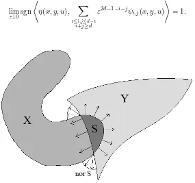
de-fined in [19, Section 2]. This are again universal differential forms like the Lipschitz-Killing curvature forms. In the special case they correspond to the mixed volumes of Section 2.1. Here η(x, y, u) is the unit simple orienting vector field of the joint normal bundle of X and Y, such that
lim
ε↓0sgn
*
η(x, y, u), X
1≤i,j≤d−1 i+j≥d
ε2d−1−i−jψi,j(x, y, u)
+
= 1.
Figure 5: Two sets X and Y with positive reach and their intersection S =X∩Y with associated normal cycle norS
Observe that the normal cycle of X∩τzY can be written as NX∩τzY = N1+ N2+N3, whereN1=NXx(intτzY ×Sd−1), N2 =NτzYx(int X×S
d−1) and N 3 =
(Hd−1xnor(∂X ∩∂(τ
simple orienting vector field ofX∩τzY andiX∩τzY(x, n) =iX(x, n)·iτzY(x, n). We use now the current version [5, 4.3.8] of the Coarea Formula 44 to conclude that N3 =π#hNX,Y, G, zi, whenever the slice is well defined.
Theorem 45. LetX, Y ⊆Rdbe two sets of positive reach. Let furtherh:R3d→Rd
be a bounded Borel measurable function with compact support supph⊂R3d. Assume
further that Ci,j(X, Y;K) is well defined for any compact set K ⊆ R2d. Then for
0≤k≤d−1 we have
Z Z
h(z, x, u)Ck(X∩τzY, d(x, u))dz
= X
i+j=k+d
Z
h(x−y, x, u)Ci,j(X, Y;d(x, y, u)). Proof. We have
Ck(X∩τzY,·) =NX∩τzY(ϕk) =N1(ϕk) +N2(ϕk) +N3(ϕk)
by the definition of the curvature measures and the additivity of normal cycles for all z ∈ Rd for which the intersection X∩τzY has positive reach. Hence, we can write the left hand side as
Z Z
h(x−y, x, u)Ck(X, d(x, u))Cd(Y, dy)
+ Z Z
h(x−y, x, u)Cd(X, dx)Ck(Y, d(y, u))
+ Z
Rd
π#hNX,Yxh, G, zi(ϕk)dLd(z) = (∗)
by using [19, Theorem 1] and the assumption of the theorem. Applying the Coarea Formula44 we get for the last integral
Z
Rd
π#hNX,Yxh, G, zi(ϕk)dLd(z)
= ((NX,Yxh)xG#Ωd)(π#ϕk) = (NX,Yxh)(G#Ωd∧π#ϕk).
Thus, by using [19, Eq. (7)] we get
(∗) = Z Z
h(x−y, x, u)Ck(X, d(x, u))Cd(Y, dy)
+ Z Z
h(x−y, x, u)Cd(X, dx)Ck(Y, d(y, u)) +
X
i+j=k+d
1≤i,j≤d−1
(NX,Yxh)(ψi,j)
= X
i+j=k+d
Z
h(x−y, x, u)Ci,j(X, Y;d(x, y, u)),
For an iterated version of the translative integral formula for sets with positive reach see [17]. In the original version of this formula, the non-osculating condition
Hd({z∈Rd:∃(x, u)∈norX,(x−z,−u)∈nor Y}) = 0
was assumed additionally. However, it was shown in [37] that this condition is not necessary to prove that reach(X ∩τzY) > 0 for almost all z ∈ Rd. It can
therefore by omitted. We further remark that Rataj [16, Thm. 1] gave an example of two (d−1)-dimensional Cd−2-submanifolds, d≥ 3, which violate the condition
Hd({z∈Rd:∃(x, u)∈norX,(x−z,−u)∈norY}) = 0.
The assumption thatCi,j(X, Y;K) is well defined for any compact setK ⊆R2d can
unfortunately not be omitted. Rataj and Z¨ahle gave an example of a compact set X⊂R4 with positive reach and u∈Sd−1, such that
H1({hx, ui: (x, u)∈norX or (x,−u)∈norX}) = 0
and the positive part of the mixed curvature measureC1,3(X, u⊥,·) is infinite on a
compact set. They also gave sufficient conditions for the assumption to hold. One of them is the following: If for any compact subsetK ⊂R4d
Z
K∩(nor X×nor Y)∩R
(sin∠(u, v))3−ddH2d−2(x, u, y, v)<+∞
then all mixed curvature measures Ci,j(X, Y;·) are well defined (this is especially
the case for d ≤ 3). Moreover, the Ci,j(X, ϑY;·)’s are well defined for almost all
rotationsϑ∈SO(d). For details and another condition involving absolute curvature measures and tangential projections we refer to [21].
4.2 The Principal Kinematic Formula
The principal kinematic formula follows now from an integration of the translative integral formula of Theorem 45 over the rotation group SO(d). Therefore we will need the following integral representation of the mixed curvature measures [19, Thm. 3.2]:
Proposition 46. For two sets of positive reachXandY inRdletaX =a1∧. . .∧ad−1
and bY = b1∧. . .∧bd−1 be unit simple orienting vector field of nor X and nor Y respectively, both having positive orientation determined by sgnhξ(x, n)∧n,Ωdi= 1, where ξ is one of the vector fields aX or bX. Let further 1≤i, j≤d−1, i+j≥d and A be a bounded Borel set of R2d. Then
Ci,j(X, Y;A) =
Z
(nor X×nor Y)∩R 1A
σ2d−1−i−j
×
is the Jacobian of the orthogonal projection of the linear subspace spanned by {ai : i ∈ I} onto the orthogonal complement of the subspace spanned by {bj : j ∈ J}, I, J ⊆ {1, . . . , d−1} and κi and λj are the generalized principal curvatures ofX andY, respectively. (αwas defined at the beginning of Section 4.1.)
By the help of this integral representation, we are now able to show the principal kinematic formula:
Theorem 47. Suppose X and Y are subsets with positive reach and A and B are bounded Borel sets of Rd. Then
Z
We now integrate both sides of the translative integral formula and obtain for the left hand side Z
SO(d)⋉Rd
Ck(X∩gY, A∩gB)dg.
For the right hand side we get Z
SO(d)
X
i+j=k+d
= X of the integral representation provided by Proposition 46 (the intersection with R can be omitted after applying ϑ, see [19, Corollary 1]) and conclude that
= X
Cj(Y, B), by using the integral representation of the generalized curvature measures
in Theorem31:
The exact value ofc′(i, j, d) may be determined by lettingXandY balls with varying radii. This leads toc′(i, j, d) =γ(i, j, d).
We can also give the following short alternative proof of the principal kinematic formula:
Proof. For fixed X and variable Y or variable X and fixedY it is easy to see that Z
SO(d)⋉Rd
is a functional as in Theorem40. Applying this result twice, we get
for some constants d(i, j, d). The exact values may again be determined by using balls with different radii.
4.3 Integral Geometry for UP R-Sets
Using the notions and notations from the last section, we will sketch now, how an integral geometry can be developed for UP R-sets. The joint unit normal bundle
nor(X, Y) of two sets X, Y ∈UP R is introduced in analogy to theP R-case:
nor(X, Y) =f#(((nor(X)×nor(Y))∩R)×[0,1]).
If it exists, the joint unit normal cycle is given by
NX,Y =f#(((NX ×NY)x1R)×[0,1]).
Once again it is guarantied NX,ϑY is well defined for almost all rotations ϑ ∈
SO(d) (cf. [20]). In this case the mixed curvature measures can be introduced: Cr,s(X, Y, A) = (NX,Yx1A×Sd−1)(ψr,s),A⊆R2d Borel. For these measures we have
whenever the integral exists (cf. [20]). This is for example the case, if X and Y belong to the convex ringR[20, Prop. 4.5]. We also have thatCr,s(X, ϑY,·) is well
defined for almost all rotationsϑ∈SO(d) [20, Prop. 4.6]. Moreover, the translative integral formula as well as the principal kinematic formula hold true and can be proved in the same way as demonstrated in the last section:
Theorem 48. Let X =SiXi, Y = SjYj be two locally finite unions of sets with positive reach in Rd. Let further h : R3d → Rd be a bounded Borel measurable
function with compact support supp h ⊂R3d. Assume further that Ci,j(X, Y;K) is
well defined for any compact set K ⊆ R2d and that for all index subsets I, J ⊂ N
non-osculating forHd-almost allz∈Rd. ThenX∩τ
zY ∈UP R for almost allz∈Rd and for 0≤k≤d−1 we have
Z Z
h(z, x, u)Ck(X∩τzY, d(x, u))dz
= X
i+j=k+d
Z
h(x−y, x, u)Ci,j(X, Y;d(x, y, u)).
By integration over SO(d) we get the principal kinematic formula forUP R-sets: Theorem 49. Suppose X, Y ∈ UP R and A and B are bounded Borel sets of Rd. Then
Z
SO(d)⋉Rd
Ck(X∩gY, A∩gB)dg =
X
i+j=k+d
γ(i, j, d)Ci(X, A)Cj(Y, B),
where γ(i, j, d) = Γ(
i+1 2 )Γ(
j+1 2 )
Γ(i+j−2d+1)Γ(d+12 ).
Remark 50. Again, using Theorem 40 one can give another short proof of this formula as in the P R-case.
The principal kinematic formula will be useful in the context of random processes of sets with positive reach and their associated union sets in Section 5.1. There, a stochastic version Theorem 49 will be derived. We also remark that the principal kinematic formula implies a Crofton-type formula for sets with positive reach as well as for locally finite unions fromUP R.
5
Random Sets with Positive Reach
As in the case of convex sets, a theory of random sets with positive reach or a theory of random processes of sets with positive reach can be developed. This general approach and concrete models will be shown within this section.
5.1 Definition and Integralgeometric Formulas
Following [31] we can construct random processes of sets with positive reach. Denote therefore byG,F,Kthe spaces of open, closed and compact sets inRd, respectively. As usual, a subbasis of the topology of F is generated by
{FG :G∈ G} ∪ {FK :K ∈ K},
where FG = {F ∈ F : F ∩G 6= ∅} and FK = {F ∈ F : F ∩K 6= ∅} (see for
{FK : K ∈ K}. Denote here by P R the family of all compact sets with positive
reach of Rd. The trace of F on P R will be denoted by PR. It was shown in [32, Prop. 1.1.1] that P R is a measurable subset of F (here we used the fact that sets with positive reach are closed).
We can now introduce random processes of sets with positive reach: Let N be the space of nonnegative, integer-valued, locally finite measures ϕ on (P R,PR). Any such measure may be represented as
ϕ(·) = X
X∈P R:ϕ({X})>0
ϕ({X})δX(·),
whereδX is the Dirac measure concentrated on X. Let furtherNbe the σ-algebra
on N, which is generated by the mappingsϕ 7→ ϕ(X) for all X ∈P R. A random point process on (P R,PR) with sample space (N,N) is now called a random process of sets with positive reach. SinceP R ∈F and F is a compact separable Hausdorff space we have that (F,F) and (P R,PR) are full (in the sense of [13]). Hence, by [13, Thm. 4], random processes of sets with positive reach can be constructed by finite dimensional distributions. We can for example construct Poissonian random processes of sets with positive reach with some given intensity measure. This will be demonstrated in Example60.
For anyϕ∈ N exists an associated union set ϕu, which is defined as
ϕu :=
[
X:ϕ({X})>0
X. (1)
As in [31, Prop. 1.3.1] we have that the mapping U : N → F : ϕ 7→ ϕu is
measurable. Hence, ϕu is a random closed set (in the sense of [12] or [14]) for any
randomP R-processϕ. To ensure thatϕu is a UP R-set, for which integralgeometric
formulas are valid, we have to restrict the class of processes to a subclass satisfying some regularity conditions. We require therefor the components of the union set ϕu to be in a general relative position. This ensures later that we can investigate
second order properties of the union set. It is clear that for anyUP R-setZ ∈UP R
there exists at least oneϕ∈ N such thatϕu =Z. We now restrict our attention to
the opposite direction, i.e. those point measures ϕ∈ N, for which ϕu ∈ UP R and
introduce the space
P Rnr :={(X1, . . . , Xn)∈P Rn:∀I ⊆ {1, . . . , n}we have
\
i∈I
Xi ∈P R},
whereP Rn=
n
×
i=1P R. Denote further byPRnthe productσ-algebra
n
O
i=1
PR
(anal-ogously then-fold product σ-algebra ofFby Fn). We have that P Rn
inPRn. The n-fold product of ϕ∈ N with itself will be denoted by ϕn. Since the
familiesP Rnr are measurable, we deduce that for eachn≥1
{ϕ∈ N :ϕn(P Rn\P Rnr) = 0} ∈N.
The space of regular processes of sets with positive reach can now be defined as
Nr=
∞
\
n=2
{ϕ∈ N :ϕn(P Rn\P Rnr) = 0}.
Definition 51. A random P R-process Φ will be called regular, if P(Φ∈ Nr) = 1. The following result is now obvious:
Proposition 52. We have Nr∈NandΦ∈ N is a regular iffP(Φn(P Rn\P Rnr) =
0) = 1for any n≥2.
For a regular P R-process Φ ∈ Nr it is now clear that its associated union set
Φu defined by (1) is a locally finite union of sets with positive reach, for which the
integralgeometric tools of Section 4.3 are available. This will be essential for the study of second order properties in the next section.
We denote by Gd = SO(d)⋉Td the group of euclidean motions, where SO(d) is
the special orthogonal group and Td the group of translations ofRd. Gd acts
nat-urally on space of sets with positive reach, namely by rotations, translations and their compositions. This action induces a natural counterpart on the space N of point measures by
gϕ(X) :=ϕ(gX),
where g ∈Gd and ϕ∈ N. Using standard arguments, one easily shows that these
actions are measurable [31, Prop. 1.7.1]
Definition 53. We say that a random P R-processΦwith distributionPΦ=P◦Φ−1 is stationary, if PΦ is invariant under all translations of Rd and isotropic, if PΦ is invariant under the action ofϑ∈SO(d) onRd. The processΦ will be called motion
invariant, if it is stationary and isotropic, i.e. invariant under all euclidean motions
g∈Gd.
Curvature measures of UP R-sets were considered in Section 3.3. We fix now a
regular random P R-process Φ, which ensures that the curvature measures of its associated union set Φu are well defined.
Mean values of curvature measures will play an important roll in the consider-ations of Section 5.2. Corresponding results and definitions are well known in the convex case.
Definition 55. Let Φ∈ Nr a regular P R-process such that
E|Ck|(Φu, B)<∞ and E|Ck|(Φt, B)<∞
for any bounded Borel setB⊆Rd, where|Ck|denotes the total variation of the
mea-sure Ck. Then the measuresCk(·) :=ECk(Φu,·) exist and are called the curvature intensity measures.
From the general result [31, Thm. 6.3.1] for signed random measures, one obtains that if Φ is stationary and Ck is determined, it is a multiple of thed-dimensional
Lebesgue measure. The proportionality factors, determined by Ck = ckLd, k =
0, . . . , d, are called curvature intensities of Φ, respectively.
We study now the intersection (and union) of processes of sets with positive reach [31, Thm. 3.1.1, Thm. 3.1.3]:
Proposition 56. Let Φ and Ψ two independent regular P R-processes and further
Φmotion invariant and Φor Ψconcentrated on compact sets. Then
(Ψ∩Φ)(·) := Z Z
δX∩Y(·)dΦ(X)dΨ(Y)
is a regularP R-process a.s. Moreover, we haveΦu∪Ψu ∈UP R and Φu∩Ψu∈UP R a.s. for their associated unions sets Φi and Ψu.
The union and the intersection of Φu and Ψu can be defined as
Φu∪Ψu :=
[
X:Φ({X})>0
X∪ [
Y:Ψ({Y})>0
Y,
Φu∩Ψu :=
[
X:Φ({X})>0
[
Y:Ψ({Y})>0
(X∩Y).
Suppose that Φ and Ψ are two independent regular random P R-processes, such that for their associated union sets we have Φu∪Ψu ∈UP R and Φu∩Ψu ∈UP R a.s.
- we say that Φu and Ψu are compatible a.s. Then the measures
Ck(Φu∪Ψu,·) = Ck(Φu,·) +Ck(Ψu,·)−Ck(Φu∩Ψu),
Ck(Φu∪Ψu,·) = Ck(Φu,·) +Ck(Ψu,·)−Ck(Φu∩Ψu)
Theorem 57. Let Φand Ψtwo independent regular randomP R-processes with the property thatΦu andΨu are compatible. Assume further that Φis motion invariant and that for any bounded Borel set B ⊂Rd
Proof. We take expectation on both sides of the principal kinematic formula for UP R-sets. The independence of Φ and Ψ yields together with Fubini’s theorem for
the right hand side
We also mention the following two important corollaries [31, Cor. 4.4 and Cor. 4.5], which are a stochastic variant of Crofton’s formula and a steriological formula for the curvature intensities:
Corollary 58. Let Φ and Ψ as in Theorem 57 and assume additionally that Ψ is stationary. Then
cΦk∩Ψ= X
i+j=k+d
γ(i, j, d)cΦi cΨj .
Corollary 59. Let E be a generic p-dimensional plane, p= 0, . . . , d−1. Then
cΦk∩E =γ(d+k−p, p, d)cΦd+k−p.
Example 60. As pointed out at the beginning of this section, randomP R-processes may be constructed via their finite dimensional distributions. We consider in this example, Poissonian P R-processes (cf. [31, Sec. 1.6]). Let therefore µ be a non-negative, locally finite measure on the space (P R,PR) and Φ∈ N such that
P(Φ(B1) =k1, . . . ,Φ(Bn) =kn) =
n
Y
j=1
(µ(Bi))kj
kj!
e−µ(Bj),
where B1, . . . , Bn are disjoint bounded sets with positive reach and k1, . . . , kn ≥ 0. Such a Φ is called PoissonianP R-process. It can now be shown [31, Sec. 5] that if
Φis a motion invariant Poissonian P R-process then Φis regular, i.e. Φ∈ Nr.
This theory will now be applied to random mosaics or random cell complexes whose cells (also the lower dimensional) are random sets with positive reach.
5.2 Random Cell Complexes and Random Curved Mosaics
In this section we apply the theory of deterministic and random sets with positive reach to random cell complexes and random mosaics in Rd. We will follow here the lines of [35] and [27]. Let thereforeMi,i= 0, . . . , d, be the space of connected
compacti-dimensional submanifoldsmiwith boundary and positive reach, i.e. mi=
mi∪∂mi and reachmi >0. By ak-dimensional cell complex inRd,p≤d, we mean
a (k+ 1)-tuple M = (M0, . . . , Mk), where for i ∈ {0, . . . , k} the Mi’s are locally
finite families fromMi (called i-cells) satisfying the incidence relations:
1. The intersection of twoi-cells fromMi is either empty or aj-cell fromMj and
j < i.
2. Any (i−1)-cell from Mi−1 is contained in the boundary of some i-cell from
Mi.
3. The boundary of any i-cell from Mi is the finite union of some (i−1)-cells
As usual in algebraic topology, the corresponding union sets ∪Mi are denoted
by |Mi| and calledi-skeletons of the cell complex M. The cells from Mk are called
k-dimensionalP R-polyhedra inRd. We now omit the smoothness conditions and let
Ui be the space of i-dimensional submanifolds with or without boundary, which are
representable asP R-polyhedra. Any (k+ 1)-tupleU = (U0, . . . , Uk) of locally finite
families ofUifromUi satisfying the incidence relations 1.-3. is called ak-dimensional
UP R-cell complex. By|Ui|we denote its i-skeleton and by|Uk|theUP R-polyhedron
associated withU.
For a stochastic model we use again the language of point processes. LetNi be the
space of locally finite, non-negative and integer-valued measures on (Ui,Ui), where Ui is the the trace of the σ-algebra UPR, which is the smallest σ-algebra for which
the mappingsf :UP R→Rd×Sd−1 :X7→closure(nor X) are measurable. The set
of atoms A(ϕi),ϕi ∈ Ni will correspond to the familyUi ofi-cells. We will identify
ϕi with A(ϕi) and write |ϕi| instead of |A(ϕi)|. The usual σ-algebra on Ni will
be denoted byNi. The space ofk-dimensional random UP R-complexes can now be
introduced as
Nk:={η= (η0, . . . , ηk) :ηi ∈ Ni, A(η) = (A(η0), . . . , A(ηk)) is aUP R−compex}.
A randomk-dimensionalUP R complex is defined as a random variableξwith values
in (Nk,Nk) (hereNkis given by (N
0⊗. . .⊗Nk)∩ N). We also writeξ = (ξ0, . . . , ξk)
as a random vector and |ξi|for the associated random i-skeleton. We call |ξk| also
the randomk-polyhedron.
For a k-dimensional UP R-complex U = (U0, . . . , Uk) the curvature measures
Cn(|Ui|,·) are well defined. The following result relates now the curvature
mea-sures of i-cells with its underlying complex (see [34, Thm. 4.2]):
Theorem 61. Let U = (U0, . . . , Uk) be a k-dimensional UP R-complex. Then for
It follows the following Euler-type relation:
Corollary 62. Under the conditions of Theorem 61we have
C0(|uk|,Rd) =
We now want to apply this theory to random cell complexes. There for we need the fact [35, Thm. 3.1.1] that for any random k-dimensional UP R-complex ξ =
(ξ0, . . . , ξk) the curvature measuresCn(|ξi|,·) are random signed Radon measures on
Rd. In analogy to Definition 53 we call a random UP R-complex ξ (defined on an abstract underlying probability space (Ω,A,P)) stationary if its distribution P◦ξ is invariant under translations ofRd. We will restrict from now on out attention to stationary random UP R-complexes which are integrable, i.e. for which
E X random cell-complex its associated mean curvature measures ECn(|ξi|,·) are multi-ples of thed-dimensional Lebesgue measures. The multiplicities (i.e. the intensities of the mean curvature measures)cin are called curvature intensities. For integrable, stationary random UP R-complexes ξ = (ξ0, . . . , ξk) the mean number Ni of i-cells
per unit volume and the shape distribution Pi of the typical cell from ξi are well
defined (cf. [35]). We denote by Cni := RCn(ui,Rd)dPi(ui) the mean value of the
1. Ci
0 is the mean Euler characteristic,
2. 2Cii−1 is the mean (i−1)-volume of the boundary and
3. Ci
i is the meani-volume of the typicali-cell of the random complexξ.
The main result for randomUP R-complexes is [35, Thm. 3.3.6]:
Theorem 63. For an integrable, stationary random UP R-complex ξ = (ξ0, . . . , ξk) in Rd we have
cin=
i
X
j=n
(−1)j−nNjCnj.
This means that the curvature intensities may be computed by the curvature properties and the mean number of the typicalj-cells,j = 0, . . . , i,i= 0, . . . , k. We can also conclude the following inversion formula:
Cni = (−1)i−n(Ni)−1(cin−cin−1). If all cells are simply connected we also have [33, Cor. 3.3.7]
Ni = (−1)i(ci0−ci0−1)
As a special case we study now random stationary mosaic of Rd. This are d-dimensional stationary random cell complexes ξ = (ξ0, . . . , ξd) (in the above sense)
with the property that|ξd|=Rd, a similar concept was studied in [27]. We remark
that this model is quite more general than the one usually used in the literature on stochastic geometry (see for example [15]).
The above formulas may be completed in the mosaic case by the relation cdd = NdCd
d = 1. Moreover the relations from above yield
d
X
j=n
(−1)j−nNjCnj = 0, n < d.
If moreover the cells are simply connected, the following Euler-type relation holds true (cf. [32, Eqn. (18)]):
d
X
j=0
(−1)jNj = 0.
Example 64. We assume that ξ is a d-dimensional integrable, stationary random mosaic in the above sense. In this case we use the following special notations: ci
k is thek-th curvature intensity of the typicali-face, Cki is the mean total k-th curvature of the typical i-face, Ni is the mean number of i-faces per unit volume, Ni,j is the man number ofj-faces adjacent to the typicali-cell, Vi,i=Ci