in PROBABILITY
COMPUTATION OF GREEKS FOR BARRIER AND
LOOK-BACK OPTIONS USING MALLIAVIN CALCULUS
EMMANUEL GOBET
Ecole Polytechnique - Centre de Math´ematiques Appliqu´ees 91128 Palaiseau Cedex - FRANCE
email: [email protected]
ARTURO KOHATSU-HIGA1
Universitat Pompeu Fabra. Department of Economics and Business. Ram´on Trias Fargas 25-27 08005- Barcelona - SPAIN
email: [email protected]
Submitted 13 November 2002, accepted in final form 31 March 2003 AMS 2000 Subject classification: 60H07, 60J60, 65C05
Keywords: barrier and lookback options, option sensitivities, Malliavin calculus
Abstract
In this article, we consider the numerical computations associated to the Greeks of barrier and lookback options, using Malliavin calculus. For this, we derive some integration by parts formulae involving the maximum and minimum of a one dimensional diffusion. Numerical tests illustrate the gain of accuracy compared to classical methods.
Introduction
In a frictionless market, let us consider a one-dimensional risky asset (St)t≥0, whose dynamic
is given, under the risk neutral probabilityP, by:
St=S0+
Z t
0
rSsds+
Z t
0
σ(Ss)SsdWs,
where ris the interest rate. We focus our attention on barrier and lookback European style options with payoff functions Φ of the type
Φ
µ
max
s∈I Ss,mins∈I Ss, ST
,
for some setI⊂[0, T]. In the following, we will sometimes omit the arguments of the function Φ = Φ(maxs∈ISs,mins∈ISs, ST) as they will be clear from the context. The form of the payoff function Φ shall remain quite general (up to the technical condition(S)below): in particular, this includes usual single and double barrier options, backward start lookback options, and in
1RESEARCH SUPPORTED BY GRANTS BFM 2000-807 AND BFM 2000-0598
each case, the risky asset can be monitored in continuous time (I = [0, T]) or discrete time (I={ti: 0≤i≤N}); we will recall later some standard examples that fit our framework. The price at time 0 of the option is equal toE(e−rTΦ) and through the paper, we are more specifically interested in computing some option derivatives (the so-called Greeks), in particular Delta ∆ = ∂S0E(e−rTΦ) and Gamma Γ = ∂2S0E(e−rTΦ), quantities related to the hedging strategy of the option. Actually, our purpose is first to derive, using an integration by parts formula of Malliavin calculus, some weightsH to rewrite each Greek above as E(e−rTΦH); and second, to apply this representation to numerically compute the Greeks and test the gain of efficiency, compared to alternative approaches such as the finite difference method (FD in short, see Glasserman and Yao [GY92], L’Ecuyer and Perron [LP94]).
In a series of recent articles (see Fourni´e, Lasry, Lebuchoux, Lions and Touzi [FLLLT99]; Fourni´e, Lasry, Lebuchoux and Lions [FLLL01]; Benhamou [Ben00]) the interest for applica-tions of the integration by parts formula of Malliavin Calculus has been increased due to the possibility of performing efficient Monte Carlo simulations to estimate the Greeks. The trick of using an integration by parts formula is natural and not very recent: Broadie and Glasserman [BG96] have introduced this idea (thelikelihood ratiomethod) when the density of the random variables involved is explicitly known. The real advantage of using Malliavin Calculus comes into play when one starts to deal with random variables whose density is not explicitly known as the case of Asian options treated in [FLLLT99] and [Ben00].
This approach using simulations of additional weights compared to FD method has proven to be efficient: the number of parameters to be chosen is smaller and the estimation is unbiased; moreover, when the payoff function is irregular, the variance of simulations is in general smaller (see the discussion in [FLLLT99]). Since for barrier options, the payoff Φ involves indicator functions, one may expect much of this method (see numerical results in section 3).
The results presented below for the computations of Greeks in the case of barrier and lookback options are new: the case of vanilla options (or depending on a finite number of dates) has been handled in [FLLLT99], whereas the case of Asian options has been systematically treated in [Ben00]. In comparison with the previous articles, here the technical difficulty comes from the lack of differentiability of the minimum and maximum processes: these random variables are only once differentiable and this is not enough to obtain in a direct way an integration by parts formula. Nevertheless, the problem of obtaining such a formula has already been considered by Nualart and Vives [NV88] where the absolute continuity of the maximum of a differentiable process is proven. More specifically, for barrier options, Cattiaux [Cat91] has performed some Malliavin calculus computations: actually, he has obtained a quasi integration by parts formula, on the time reversed process; unfortunately, although these formulae are useful for theoretical purposes, they are difficult to use in practice for the Greeks. Later in Nualart [Nua95], the smoothness of the density of the supremum of the Wiener sheet is obtained: for this, he uses a localization procedure. We will adapt this idea in our situation, using a dominating process, which controls the extrema of (St)0≤t≤T. Another technical issue is what are the elements that determine a good dominating process. Here, we propose two. One is the extrema of the process and another is obtained through Garsia-Rodemich-Rumsey’s Lemma. The choice of the dominating process has effects on the size of the program to compute the Greeks. For this reason, we have studied numerically the behavior of these two dominating processes.
Concerning the Malliavin calculus, we use the notations and definitions that are standard in this area and that can be found in e.g. [Nua95].
Preliminaries
For the sake of simplicity, we are going to consider a transformation of S which avoids some degeneracy problems on the diffusion coefficient, i.e. Xt = A(St) where A is the strictly increasing functionA(y) =Ry
1 du
uσ(u),so that
Xt=x+
Z t
0
h(Xs)ds+Wt. (1)
where x=A(S0) and h(u) = (r/σ(y)−(yσ(y))′/2)|
y=A−1(u). This corresponds to the usual logarithm change in Black & Scholes model. In the following, we will assume thathis aC∞
b function. If we denote Mt= maxs≤t,s∈IXs andmt= mins≤t,s∈IXs, the main issue consists in expliciting Malliavin integration by parts formula for ∆ and Γ, which are related to (up to the discounted factor and the change of variables)
∂xE(Φ(MT, mT, XT)) =E(Φ(MT, mT, XT)H1)
∂2x,xE(Φ(MT, mT, XT)) =E(Φ(MT, mT, XT)H2)
for some random variablesH1andH2. In the following, the payoff Φ(MT, mT, XT) is supposed to be squared integrable. Furthermore, we impose a support type condition on Φ
(S) There existsa >0 such that the function Φ(M, m, z) does not depend on the variables (M, m) for any (M, m, z) such that 0≤M −x < aor 0≤x−m < a.
If only the maximum M (resp. the minimum m) is involved in the Pay-Off, the above as-sumption shall be implicitly rewritten omittingm (resp. M): in the first case,(S) is stated as
(S)For somea >0, the function Φ(M, z) does not depend onM if 0≤M−x < a. and in the second one,
(S)For somea >0, the function Φ(m, z) does not depend onm if 0≤x−m < a.
These technical conditions are actually not so restrictive: it includes all usual barrier options and most of lookback ones. Let us give some examples, where the parametera >0 is given.
• Single barrier options.
– Up & out barrier : Φ(M, m, z) =1 M <U f(z) withx < U. Takea=U −x. – Down & in barrier : Φ(M, m, z) =1 m≤Df(z) withD < x. Takea=x−D.
• Double barrier options (D < x < U).
– Double out barrier: Φ(M, m, z) =1 M <U 1 m>Df(z). For the same arguments as before, results will apply witha= min(U−x, x−D).
• Backward start lookback Put: Φ(M, m, z) = max(M0, M)−z, with M0 > x. Take
a=M0−x.
• Out of money Put on minimum: Φ(M, m, z) = (K−m)+, withK < x. Takea=x−K.
1
Computation of the delta and gamma
1.1
Assumptions and notations
Our general approach consists in assuming that there exists an non-decreasing adapted right-continuous process (Yt)0≤t≤T such that:
∀t∈I |Xt−x| ≤Yt. (2)
We shall call ita process dominating X or anX-dominating process.
Remark 1.1. If the maximum and the minimum were computed on different time sets I
and J, our results stated below would be true, still under (S), taking a dominating processY
relatively to the bigger time set I∪J.
We assume that the following estimate holds true.
(H) There exists a positive functionα:N7→R+, with limq
→∞α(q) =∞, such that, for any
q≥1, one has: ∀t∈[0, T] E(Ytq)≤Cqtα(q).
In particular, one hasY0= 0. Furthermore, we shall expectY to be somewhat smooth in the Malliavin sense. For this, choose aC∞
b function Ψ : [0,∞)7→[0,1], with Ψ(x) = 1 ifx≤a/2, and 0 if x≥a: the real positive numberais the one appearing in the support condition(S). Forq∈N∗, consider the following regularity assumption:
(R(q)) The random variable Ψ(Yt) belongs toDq,∞for eacht. Moreover, forj= 1,· · ·, q, one
has
∀p≥1 sup
r1,···,rj∈[0,T] E
Ã
sup r1∨···∨rj≤t≤T
|Dr1,···,rjΨ(Yt)|p
!
≤Cp.
Moreover, for q ≥ 2, the q−1 first derivatives of Ψ(Yt) w.r.t. x, i.e. ∂x(Ψ(Yt)),· · · , ∂q−1
x (Ψ(Yt)), exist and satisfy the same estimates as above.
The construction of the process (Yt)0≤t≤T will be done later in section 2. Actually, it can depend on the type of subsetI.
We will carry out the Malliavin calculus computations on the extrema of (Xt)t∈I if X is a Brownian motion without drift (or with a deterministic one): up to a change of probability measure, we can reduce our problem to this. Consider
ZT =
dP
dQ
¯ ¯ ¯ ¯F
T
= exp¡ Z T
0
h(Xs)dVs− 1 2
Z T
0
which defines the measure Q, under which (Vt)t≥0 = (Xt−x)t≥0 is a standard Brownian motion. Thus, one has:
EP(Φ(MT, mT, XT)) =EQ(Φ( max
s≤T,s∈IVs+x,s≤minT,s∈IVs+x, VT +x)ZT). (3) Hence, the derivation of formulae for the Greeks can be performed underQand then, rewritten underP: for simplicity of notation, we leave final formulae expressed under Q.
If for anyt∈I∩[0, T] the random variableUtbelongs to D1,2, it is well known that, under some additional mild conditions (see Nualart and Vives [NV88] for a precise statement), the random variables mins≤T,s∈IUs and maxs≤T,s∈IUs also belong to D1,2. The next lemma develops this result whenU is a standard Brownian motion with a non random drift.
Lemma 1.1. Let V be a standard Brownian motion and consider Vtf =Vt+R t
0f(s)ds, for a deterministic function f. Then, the random variables mins≤T,s∈IVsf and maxs≤T,s∈IVsf belongs toD1,∞ and their first weak derivatives are defined as follows: fort∈[0, T], one has
Dt
Actually,τmandτM are uniquely defineda.s.(see Karatzas and Shreve [KS91]). Note that the random variables mins≤T,s∈IVsand maxs≤T,s∈IVsdo not belong to D2,p, so that a classical integration by parts formula can not apply for them. Nevertheless, a localization procedure using the dominating processY will give some results (some analogous situations are handled in Nualart [Nua95], Proposition 2.1.5).
1.2
Integration by parts formulae
We now state the main results of the paper.
Theorem 1.1. Assume (S)and(H). 1) IfY satisfies(R(1)), set H1=δ
+∂xZT (the explicit expression for
∂xZT is given in the proof below). Then, one has
where ∂xZT =ZT R0Th′(x+Vs)(dVs−h(x+Vs)ds).The weak derivative of Φ is equal to
DtΦ = Φ′M1t≤τM+ Φ′m1t≤τm+ Φ′z,
using the notation from Lemma (1.1). The key point is to remark that one has
DtΦ Ψ(Yt) = (div Φ)( max
s≤T,s∈IVs+x,s≤minT,s∈IVs+x, VT +x)Ψ(Yt). (7) Indeed, due to the condition(S), both sides of the above expression equal Φ′
zΨ(Yt) on the event
A={maxs≤T,s∈IVs≤a} ∪ {mins≤T,s∈IVs≥ −a}. OnAc and fort such that Ψ(Yt)6= 0, one hasYt< a; hence using (2), one has maxs≤t,s∈IVs< a <maxs≤T,s∈IVs and mins≤t,s∈IVs>
−a >mins≤T,s∈IVs, that ist≤τM andt≤τm. This proves that, onAc, one has
1t≤τMΨ(Yt) = Ψ(Yt) and 1t≤τmΨ(Yt) = Ψ(Yt).
From (7), it readily follows, using the integration by parts of Malliavin Calculus (formula (1.41) from Nualart [Nua95]) since Ψ(Yt) is smooth and satisfies(R(1)), that
EQ
The above computations are valid up to verifying that (RT
0 Ψ(Yt)dt)
2.3.1 in [Nua95]). Due to the non-decreasing property ofY, this probability is upper bounded byP(a/2< Yǫ)≤ EP(Yǫq)
(a/2)q ,and the conclusion follows from assumption(H). The combination of (6) and (8) leads to the required expression forH1.
2) Formula forΓ. We remark that the smooth random variableZT in (3) for the computation of ∆ has been replaced by the smooth random variableH1 in (4). Hence, the derivation ofH2 is straightforward.
It is worth noticing that formulae from Theorem (1.1) can be simplified when the drift function
h(x) in (1) is constant equal toµ(this includes the Black & Scholes model): in that situation,
X is, under P, a Brownian motion with deterministic drift, so that Lemma (1.1) directly applies and no change of measure is needed. Hence, one obtains the
Theorem 1.2. Assume (S)and(H)and suppose thatXt=x+Wt+µ t.
2
Construction of dominating processes
Y
Until now, we have assumed the existence of a dominating processY satisfying some regularity assumptions and some estimates. In this section, we explicit these processes in two cases.
1) I is the full interval [0, T].
2) I consists in a finite number of times.
The first case corresponds to continuous time monitored barrier and lookback options, and the second, to discrete time ones. These two cases include most standard situations that appear in practice.
Note that any dominating process for X in the case I = [0, T] is also a dominating process for any case I ⊂ [0, T]; however, its numerical efficiency may not be optimal as shown in the section of numerical simulations. Throughout this section,X is the solution of the SDE (1), although the results in this section are also valid ifX were one component of a general multidimensional diffusion process.
2.1
The case of continuous time maximum/minimum:
I
= [0
, T
]
2.1.1 Extrema process
The simplest dominating process is probably the extrema process
Yt= max
s≤t(Xs−x)−mins≤t(Xs−x).
It is easy to check that it satisfies (2), assumptions(H)and(R(1)). Hence, the computation of ∆ can be performed using formula (4) or (9) with such a dominating process.
However, sinceYtdoes not belong toD2,p, one needs smoother dominating process to compute Γ and higher sensibilities. That is what we develop now.
2.1.2 Averaged modulus continuity process For an even integerγ, define
Yt:= 8
µ
4
Z t
0
Z t
0
|Xs−Xu|γ
|s−u|m+2 ds du
¶1/γm+ 2
m t
m/γ. (11)
Using the classical estimates E(|Xs−Xu|γ)≤Cq|s−u|γ/2, one remarks that the condition 0 < m < γ2 −2 implies that E³Rt
0
Rt
0
|Xs−Xu|γ
|s−u|m+2 ds du
´
< ∞, so that (Yt)0≤t≤T is a.s.well defined. This process is clearly non-decreasing, adapted and continuous; the next lemma justifies thatY is a good candidate for our procedure.
Lemma 2.1. Let γbe a even integer and set msuch that 0< m < γ2−2. Then, one has: i) For any t∈[0, T], one has|Xt−x| ≤Yt.
ii) The assumption(H) is satisfied.
Proof. Assertion i) is a consequence of Garsia-Rodemich-Rumsey’s Lemma [GRR70]. Indeed,
Assertion ii) is easy to prove using classical estimates on the modulus of continuity of SDEs: we omit the details.
Proof of Assertion iii). We prove the estimates for Ψ(Yt), those for its derivatives w.r.t. x
being similar. Standard computations (see Chapter 2.2, Nualart [Nua95]) prove that, for any
t∈[0, T],Bt∈Dq,∞ ifq≤γ−2(m+ 2). Moreover, forj = 1,· · · , q, one has
In that situation, to find dominating processes with good properties is much easier than for the continuous case. As before, the extrema process Yt = max0≤i≤N:ti≤t(Xti −x)− min0≤i≤N:ti≤t(Xti−x) is still valid, only for the computation of ∆: it clearly satisfies (2), assumptions(H)and(R(1)).
For higher sensibilities, following the idea of using the averaged modulus continuity process from Garsia-Rodemich-Rumsey’s Lemma, let us consider the non-decreasing, adapted and right-continuous process ii) The assumption(H)is satisfied.
iii) For any q≥1, assumption(R(q))is satisfied.
Proof. Fort=tj, one has|Xt−x| ≤Pi=1j |Xti−Xti−1| ≤Yt,using Jensen’s inequality: this proves Assertion i). Others assertions are also easy to justify, we omit the details.
3
Numerical results
-0.1 -0.05 0 0.05 0.1 0.15
0 1000 2000 3000 4000 5000 6000 7000 8000 9000 10000 True Value
FD Malliavin
Figure 1: Delta of an up & out Call, using the averaged modulus continuity process.
cases closed formulae for the Greeks: these values are taken as references for some of our numerical tests.
On figure 1, we represent some results of the numerical computation of the Delta for a con-tinuous time monitored up & out Call, with upper barrierU = 120 and StrikeK = 100 (the
x-range correspond to the number of simulations). We compare the standard Finite Difference method (FDplot) (see [LP94]), and our Malliavin calculus approach (Malliavinplot) (i.e. for-mula (9), up to the logarithm change and to the discounting factor). For the second method, we here use the averaged modulus continuity process (11) as the X-dominating process: the involved parameters have been taken here equal toγ= 20 andm= 3, but other values merely lead to same qualitative results.
-0.16 -0.14 -0.12 -0.1 -0.08 -0.06 -0.04 -0.02 0 0.02
0 1000 2000 3000 4000 5000 6000 7000 8000 9000 10000 True Value
FD Malliavin
Figure 2: Gamma of an up & out Call.
Figure 2 corresponds to the computation of the Gamma, with the same parameters.
-0.02 -0.015 -0.01 -0.005 0 0.005 0.01 0.015 0.02
0 1000 2000 3000 4000 5000 6000 7000 8000 9000 10000 True Value
FD Malliavin
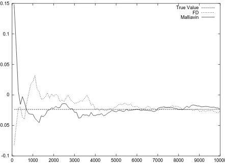
Figure 3: Delta of an up & out Call, using the extrema process.
values for the mean and the standard deviation (in bracket) of the procedures for N= 10000 paths.
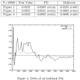
N=10000 True Value FD Malliavin
Figure 1 -0.0237 -0.0269(0.0116) -0.0235(0.0097) Figure 2 -0.0055 -0.0041(0.0233) -0.0063(0.0014) Figure 3 -0.0105 -0.0092(0.0035) -0.0096(0.0097)
-0.6 -0.58 -0.56 -0.54 -0.52 -0.5 -0.48 -0.46 -0.44
0 1000 2000 3000 4000 5000 6000 7000 8000 9000 10000 True Value
FD Malliavin
Figure 4: Delta of an lookback Put.
is smaller.
We now consider the example of a backward start lookback Put with M0 = 130. Figure 4 presents the result for the FD and Malliavin methods (the latter being performed with the extrema process). Here, we observe that the variance for the second method is much higher than for the FD one: this may be explained by the fact that the payoff is merely smooth w.r.t. S0. This phenomena is well-known and occurs e.g. for the Vanilla Call, for which a local integration by parts formula shall be performed (see [FLLLT99]). We do not investigate furthermore in that direction.
0.01 0.015 0.02 0.025 0.03 0.035 0.04 0.045 0.05
0 1000 2000 3000 4000 5000 6000 7000 8000 9000 10000 True Value
FD Malliavin FLLLT99
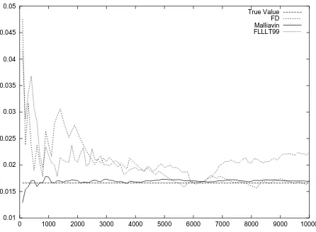
Figure 5: Delta of up in & down out digital Call.
Another interesting example is discrete time monitored barrier options. Let us consider a daily monitored up in & down out digital Call, with upper barrierU = 130, lower barrierD = 70 and strikeK= 100. Note that here, no closed formula is available for the price of the option and its Greeks, so the True Valuein Figure 5 is obtained using FD method with very large number of simulations. Since the payoff function
Φ =1 min1≤i≤250Sti>D 1 max1≤i≤250Sti≥U 1 ST≤K
involves only a finite number ofSti, results from [FLLLT99] can be applied. We find that
∆ =E
µ
e−r T Φ Wt1
σ S0t1
.
Hence, we can compare the results using this formula (FLLLT99plot), FD method and our approach: this is achieved on Figure 5.
N=10000 True Value FD Malliavin FLLLT99
Figure 5 0.0166 0.0171 (0.0028) 0.0168(0.0004) 0.0222 (0.0033)
4
Conclusion
In this paper, Malliavin calculus integration by part formulae have been performed for the maximum and minimum of a one dimensional diffusion: the key argument is to introduce an extra dominating process, which localizes Malliavin calculus computations, avoiding some problems with the lack of differentiability of the maximum and minimum processes.
These computations lead to new formulae for the Delta and Gamma of barrier and lookback options, in a continuous or discrete setting.
Numerical tests illustrates that this approach can give more accurate results than with FD method, when the complexity is a bit more important. In particular, in the discrete time case, the method is much more efficient than FD method or that from [FLLLT99].
Acknowledgements. We would like the anonymous referee for his valuable suggestions.
References
[Ben00] E. Benhamou. An appplication of Malliavin calculus to continuous time Asian Options’Greeks. Technical report, London School of Economics, 2000.
[BG96] M. Broadie and P. Glasserman. Estimating security price derivatives using simula-tion. Management Science, 42(2):269–285, 1996.
[Cat91] P. Cattiaux. Calcul stochastique et op´erateurs d´eg´en´er´es du second ordre - II. Probl`eme de Dirichlet. Bull. Sc. Math., 2`eme s´erie, 115:81–122, 1991.
[FLLLT99] E. Fourni´e, J.M. Lasry, J. Lebuchoux, P.L. Lions, and N. Touzi. Applications of Malliavin calculus to Monte Carlo methods in finance. Finance and Stochastics, 3:391–412, 1999.
[FLLL01] E. Fourni´e, J.M. Lasry, J. Lebuchoux, and P.L. Lions. Applications of Malliavin calculus to Monte Carlo methods in finance, II. Finance and Stochastics, 5:201–236, 2001.
[GRR70] A.M. Garsia, E. Rodemich, and H.Jr. Rumsey. A real variable lemma and the continuity of paths of some gaussian processes. Indiana University Mathematics Journal, 20(6):565–578, 1970.
[GY92] P. Glasserman and D.D. Yao. Some guidelines and guarantees for common random numbers. Management Science, 38(6):884–908, 1992.
[KS91] I. Karatzas and S.E. Shreve. Brownian motion and stochastic calculus. Second Edition, Springer Verlag, 1991.
[LP94] P. L’Ecuyer and G. Perron. On the convergence rates of IPA and FDC derivative estimators. Oper. Res., 42(4):643–656, 1994.
[Nua95] D. Nualart. Malliavin calculus and related topics. Springer Verlag, 1995.