E l e c t ro n ic
Jo u r n
a l o
f P
r o b
a b i l i t y
Vol. 6 (2001) Paper no. 15, pages 1–13. Journal URL
http://www.math.washington.edu/~ejpecp/ Paper URL
http://www.math.washington.edu/~ejpecp/EjpVol6/paper15.abs.html
ON DISAGREEMENT PERCOLATION AND MAXIMALITY OF THE CRITICAL VALUE
FOR IID PERCOLATION Johan Jonasson
Dept. of Mathematics, Chalmers University of Technology, S-412 96 Sweden [email protected]
AbstractTwo different problems are studied: (1) For an infinite locally finite connected graph G, letpc(G) be the critical value for the existence of an infinite cluster in iid bond percolation
on Gand letPc = sup{pc(G) :G transitive, pc(G)<1}. IsPc <1?
(2) Let Gbe transitive with pc(G)<1, let p∈[0,1] and letX and Y be iid bond percolations
onG with retention parameters (1 +p)/2 and (1−p)/2 respectively. Is there aq <1 such that p > q implies that for any monotone coupling ( ˆX,Yˆ) of X and Y the edges for which ˆX and
ˆ
Y disagree form infinite connected component(s) with positive probability? Let pd(G) be the
infimum of such q’s (includingq= 1) and let Pd= sup{pd(G) :Gtransitive, pc(G)<1}. Is the
stronger statement Pd<1 true? On the other hand: Is it always true that pd(G)> pc(G)?
It is shown that if one restricts attention to biregular planar graphsGthen these two problems can be treated in a similar way and all the above questions are positively answered. We also give examples to show that if one drops the assumption of transitivity, then the answer to the above two questions is no. Furthermore it is shown that for any bounded-degree bipartite graph Gwithpc(G)<1 one has pc(G)< pd(G).
Problem (2) arises naturally from [6] where an example is given of a coupling of the distinct plus- and minus measures for the Ising model on a quasi-transitive graph at super-critical inverse temperature. We give an example of such a coupling on ther-regular tree,Tr, for r≥2.
Keywords coupling, Ising model, random-cluster model, transitive graph, planar graph AMS Subject Classification60K35, 82B20, 82B26, 82B43
1
Introduction
Let G = (V, E) be an infinite locally finite connected graph. (For the rest of this paper all graphs are assumed to have these properties if nothing else is explicitly stated.) Let pc(G) be
the critical value for the existence of an infinite cluster for iid bond percolation onG. Then for anyp∈[0,1] one can designG(e.g. by considering a properly chosen spherically symmetric tree, see e.g. [9]) in such a way thatpc(G) =p. In particular one can have pc(G) <1 but arbitrarily
close to 1. An example of a sequence {Gn} of graphs such that pc(Gn) < 1 and pc(Gn) ↑ 1
is constructed by letting Gn be a binary tree with each edge replaced by an path of length n.
However, if Gis required to betransitive, i.e. if the automorphism group of G acts transitively on V, then this does not seem to be the case. We have
Conjecture 1.1 Let Pc = sup{pc(G) :Gtransitive, pc(G)<1}. ThenPc <1.
This was first stated by Olle H¨aggstr¨om (private communication). (One should note that there are of course transitive graphsGwithpc(G) = 1 even with arbitrarily high degree.)
We shall prove Conjecture 1.1 for a large class of planar graphs, i.e. graphs which can be embedded in the plane in such a way that no two edges cross. From now on we assume that a planar graph is embedded in such a way. For a planar graph G its planar dual is the planar (multi)graph G† = (V†, E†) where V† is the set of faces of G and two faces are joined by an edge inE† precisely when they share an edge inE. Note that when the minimal degree inGis at least 3 then G† is a graph. A graphG is said to be regular if all its vertices have the same degree and in this case we denote the common degree by dG. If G is planar and regular and
such thatG† is also regular then we say thatGisbiregular. In this caseGis also transitive, see [8]. We will prove:
Theorem 1.2 Let Pcplb = sup{pc(G) : G planar and biregular, pc(G) < 1}. Then Pcplb ≤
√
5/(1 +√5).
The proof is given in Section 3.
Let us now for a while turn to the second question of this paper. van den Berg [3] introduced the concept ofdisagreement percolation as a tool to prove Gibbsian uniqueness for Markov random fields: If X1 and X2 are picked independently according to two Gibbs measuresµ1 and µ2 for the same specifications of a Markov random field on SV, where S is some finite set, and P(G
Theorem 1.3 Let r ≥ 2, let G = Tr, the r+ 1-regular tree and let βc be the critical inverse temperature for the existence of multiple Gibbs mesures for the Ising model on G. Then there exists βd> βc such that for all β ∈(βc, βd) there is a coupling ( ˆX1,Xˆ2) of X1 andX2 (defined on a probability space with underlying probabilty measure P), where X1 and X2 are distributed according to the minus- and plus Gibbs measures respectively, such thatP(there exists an infinite connected component of disagreements between Xˆ1 and Xˆ2) = 0.
An example that proves Theorem 1.3 is given in Section 5.
In light of Theorem 1.3 many questions arise naturally. For example: Could Tr be replaced by any transitive graph G with pc(G) < 1? Could β be arbitrarily large or must it be close
to βc? Is the set of β’s for which such a coupling exists an interval? What if one considers
Potts models with more than two different spins? Could one replace Tr by the integer lattice Z
d? However, when considering questions of this sort there is no particular reason to restrict
oneself to Ising/Potts models. Indeed one could ask these or similar questions about virtually any percolation process. However in order to make the problems precise one has to choose a model to work with. We shall instead of working with the Ising/Potts model make what seems the most natural choice and use the “cleanest” percolation process as our testing ground, namely iid (bond) percolation. We shall ask:
• Is there a graph G for which for any p ∈ [0,1], iid (bond) percolation with retention parameter (1 +p)/2 can be coupled to iid percolation with retention parameter (1−p)/2 with a.s. no infinite cluster of disagreement?
and the natural reverse question:
• If (1 +p)/2−(1−p)/2 =p < pc(G) then by coupling the two processes via independent
edge-wise maximal couplings, there will a.s. be no disagreement percolation. Is there any Gfor which this is indeed the best one can do?
In the second case it is not hard to see that for many Gone can do better than just edge-wise maximal couplings. For example when G=T2, the binary tree, one can by dividing the edges into properly chosen “families” construct a coupling without disagreement percolation even when p is slightly larger than 3/4 (indeed, as it turns out the coupling in Section 5 is more or less a coupling of this kind, but for site percolation) and as we shall see below that this idea works in much larger generality.
We believe that the answers to the two questions are no in general, as long as we stick to “nice enough” graphs:
Conjecture 1.4 If G is transitive and pc(G) < 1 then there exists a q < 1 such that if
p > q then any coupling of iid-percolation(p) with iid-percolation(1-p) produces with positive probability an infinite cluster of disagreements. Moreover, withpd(G) being the infimum of such
q′s(including q= 1) and Pd= sup{pd(G) :G transitive, pc(G)<1}, we have Pd<1.
If we drop the assumption of transitivity, then the first part of the conjecture is false. Indeed in Section 4 we give a counterexample where G haspc(G) = 0 andpd(G) = 1. For the second
part with the assumption of bounded degree dropped we do not know the answer. In Section 4 we also prove the following partial confirmation of Conjecture 1.4. Before stating it we need the definition of a bipartite graph: The graph G = (V, E) is said to be bipartite if V can be partitioned into Vo ∪Ve, the sets of odd vertices and even vertices respectively, such that
u∈Vo,(u, v) ∈E ⇒v∈Ve and u ∈Ve,(u, v) ∈E ⇒v ∈Vo. Note that a graph is bipartite iff
all its cycles are of even length. This applies to many of the commonly studied graphs, e.g.Z
d,
the hexagonal lattice and all trees (but not to the triangular lattice though).
Theorem 1.5 (a) Let Gbe planar and biregular withpc(G)<1. Then pd(G)<1. Moreover,
withPdplb= sup{pd(G) :G planar and biregular, pc(G)<1}, we have Pdplb<1.
(b) Let G be a bounded-degree bipartite graph with pc(G)<1. Thenpd(G)> pc(G).
2
Preliminaries
The (egde-)isoperimetric constantof a graph G= (V, E) is defined as
κ(G) = inf{|∂EW|
|W| :W ⊂V,|W|<∞}
where∂EW is the outer edge boundary ofW, i.e. the set of edges with one endpoint in W and
one endpoint in V \W. If κ(G) = 0 then Gis said to be amenable and if κ(G) >0 then G is said to benonamenable.
When Gis transitive we have from [1] thatκ(G) coincides with
κ′(G) = lim inf
N→∞{ |∂EW|
|W| :W connected, N <|W|<∞}.
In general we have κ(G) ≤κ′(G). If Gis nonamenable thenpc(G)<1. Indeed, Benjamini and
Schramm [2] show that:
Lemma 2.1 pc(G)≤1/(1 +κ′(G)).
We will use this along with the following formula from [8] (Theorem 4.1):
Lemma 2.2 Let Gbe planar and biregular with dual G† and assume that dG† <∞. Then
κ(G) = (dG−2) s
1− 4
(dG−2)(dG† −2) .
In case G† is not regular the formula of Lemma 2.2 has no meaning. We believe that if d
G† is replaced with the harmonic average of the numbers of edges of thedG different faces ofGthat
ourselves to planar biregular graphs instead of all planar transitive graphs in Theorems 1.2 and 1.5(a). If our belief holds then these theorems would extend in a straightforward way to the class of all planar transitive graphs.
We will also need the following result of Kesten [11]:
Lemma 2.3 Let G be a regular graph and for n= 1,2, . . . and v∈V, let Cn(v) be the number
of connected subsets of nvertices that contain v. Then
Cn(v)≤(edG)n.
Finally before moving on to the main sections we need to introduce the concept of stochastic domination. Let (S,S) be some measurable partially ordered space. An event A ∈ S is said to be increasing if x ∈A, x≤y ⇒ y ∈A. If µ and ν are two probability measures on S then we say that µ is stochastically dominated by ν if µ(A) ≤ ν(A) for every increasing event A and in this case we writeµ ≤dν. If X and Y are S-valued random variables distributed to µ and
ν respectively, then we say that X is stochastically dominated by Y and write X ≤d Y. By
Strassen’s Theorem µ≤dν is equivalent to the existence of a coupling ( ˆX,Yˆ) ofX andY such
thatX ≤Y a.s.
3
Maximality of
p
c(
G
)
Proof of Theorem 1.2. In order to prove Theorem 1.2 we first take care of the cases when dG† =∞, i.e. when Gis a regular tree. Then if dG = 2 we have pc(G) = 1 and if dG ≥3 then κ(G) =dG−2 andpc(G) = 1/(dG−1) as is well known.
Assume second that 7≤dG† <∞. Then by Lemma 2.2 we have
κ(G) = (dG−2) s
1− 4
(dG−2)(dG† −2) ≥ 1/√5
and so by Lemma 2.1, pc(G)≤√5/(1 +√5).
IfdG† ∈ {5,6}anddG≥4 then again by Lemma 2.2,κ(G)≥2/ √
3 so thatpc(G)≤
√
3/(2+√3). For dG† = 4 and dG ≥ 5 we get similarly that κ(G) ≥
√
3 and pc(G) ≤ 1/(1 +√3) and for
dG† = 3 anddG≥7 we get κ(G)≥ √
5 andpc(G)≤1/(1 +√5).
The only remaining cases are now the square, triangular and hexagonal lattices for whichpc(G)
is 1/2, 2 sin(π/18) and 1−2 sin(π/18) respectively. (Note that if dG = 3 and dG† ≤5 or vice versa thenGis finite.)
Summarizing we have seen thatPcplb≤√5/(1 +√5)<0.7, proving Theorem 1.2. ✷
Remark. By considering all “standard” examples of nonamenable transitive graphs it is easy to believe that if one puts K = inf{κ(G) : G transitive and nonamenable}, then K > 0. In light of Lemma 2.1 this would then have implied an analog to Theorem 1.2 for the class of all nonamenable transitive graphs. However it turns out thatK = 0. This was recently established by Grigorchuk and de la Harpe [5] who construct a sequence {Gn} of nonamenable Cayley
graphs such that κ(Gn)↓ 0. The sequence {Gn} is of course a candidate for a counterexample
4
Disagreement percolation
4.1 Proof of Theorem 1.5(a)
LetG= (V, E) be a graph and letXandY be bond percolations onGwith retention parameters (1 +p)/2 and (1−p)/2 respectively. We saw in the proof of Theorem 1.2 above that if G is any planar biregular graph other than the square, triangular or hexagonal lattice, then G is nonamenable with κ(G) ≥1/√5. Indeed Lemma 2.2 tells us that for all these graphs we have κ(G) ≥κ0dG whereκ0 = (3√5)−1. Now let ( ˆX,Yˆ) be an arbitrary coupling of X and Y with underlying probability measure P. Fix a positive integer m and a connected set K ⊂ V with |K|=m. In order for no vertex v∈K to be in an infinite cluster of disagreements between ˆX and ˆY there must be some positive integer n and some connected W ⊂V such that |W|=n, W ⊇K and such that ˆX and ˆY agree on every edge of∂EW. However
P( ˆX(∂EW)≡Yˆ(∂EW))≤P(|Xˆ(∂EW)| ≤n/2) +P(|Yˆ(∂EW)| ≥n/2)
= 2P(|Xˆ(∂EW)| ≤n/2).
Since |Xˆ(∂EW)| has a binomial distribution with parameters |∂EW| and p, a standard tail
estimate in the binomial distribution yields for some constantC (depending onp)
P( ˆX(∂EW)≡Yˆ(∂EW))≤2C
n ⌊n/2⌋
2−n(1 +p)⌈n/2⌉(1−p)⌊n/2⌋
≤2C(1−p2)n/2.
Summing over n and all W’s with |W|=n, using Lemma 2.3 applied with v being any vertex of K, we get
P(Nov∈K is in an infinite cluster of disagreements between ˆX and ˆY)
≤2C
∞
X
n=m
(edG)n((1−p2)κ0dG/2)n
which is less than 1 for large enough mas soon as
edG(1−p2)κ0dG/2<1
i.e. as soon as
p2≥1− 1
(edG)2/(κ0dG)
= 1− 1
(edG)6
√ 5/dG
.
The “worst case” is whendG = 3 in which case we get thatpd(G) is bounded above by
s
1− 1
(3e)2√5
which is less than 0.9999581.
(Note also that asdG → ∞we get thatpd(G) =O( p
logdG/dG) which can be compared to the
Now assume thatGis one of the square lattice, the triangular lattice and the hexagonal lattice. In each of these case we have dG† ≤ 6, so for each integer n the number of cutsets (i.e. edge boundaries of finite connected subsets ofV containingK) of sizenis bounded byn5n. By using
the same arguments as above we get that
P(Nov∈K is in an infinite cluster of disagreements between ˆX and ˆY)
≤2 ∞
X
n=m
n5n((1−p2)1/2)n
which is less than 1 for large enough mas soon as
p≥ √
24 5 . Thuspd(G)≤
√
24/5<0.9798. Theorem 1.5(a) follows withPdplb<0.9999581. ✷
4.2 A non-transitive counterexample
Now we shall drop the assumption of transitivity and see that we can construct aGwithpc(G) =
0 such thatX and Y can for anyp be coupled without an infinite cluster of disagreements. A graphGis said to be a spherically symmetric tree if it is a tree and if for some vertexv∈V it is the case that for every positive integer n all vertices at graphical distance n from v have the same degree. The vertexv is called a root of G. Now let Gbe a spherically symmetric tree specified in the following way: Let a vertexo, which is to be the root, have degree 3. Letdn be
the degree of vertices at distance nfrom oand let {d1, d2, d3, . . .}
={3,2,4,4,2,2,5,5,5,2,2,2,6,6,6,6,2,2,2,2,7,7,7,7,7,2,2,2,2,2, . . .}.
Then a simple branching process argument shows thatpc(G) = 0. However, all infinite connected
paths inG contain arbitrarily long induced paths, i.e. paths containing only vertices of degree 2. For a given p let N be the smallest integer such that ((1 +p)/2)N ≤ 1/2 and assume for simplicity that ((1 +p)/2)N = 1/2. Now for an edge e not in an induced path containing
at least N edges, let ( ˆX(e),Yˆ(e)) be independent of ( ˆX(E\ {e}),Yˆ(E \ {e})) and such that ˆ
X(e) ≥ Yˆ(e). For an induced path W containing at least N edges, let E(W) be its set of edges and let E(W) = E1 ∪E2 where E1 consists of the N edges that are nearest to o and E2 =E(W)\E1. For e∈E2, couple ˆX(e) and ˆY(e) independently of all other edges like for the edges not in long induced paths above. For E1, let ˆX(E1)≡ 1 iff ˆY(E1)6≡ 0. This is possible since ((1 +p)/2)N = 1/2. Couple all induced paths containing at least N edges independently
of each other in this way. Now since each such induced path contains at least one edge for which ˆ
X(e) = ˆY(e) it follows that no infinite cluster of disagreements can exist.
Finally if ((1 +p)/2)N < 1/2, then minor modifications which are left to the reader yields a monotone coupling where ˆX(E1)≡1⇒Yˆ(E1)6≡0.
Remark. The above example was constructed so that pc(G) = 0 in order to be as spectacular
4.3 Proof of Theorem 1.5(b)
LetQbe the probability measure that underlies the coupling (X′, Y′) ofXandY via independent edge-wise maximal couplings, i.e. for which Q(X′(e) = Y′(e) = 1) =Q(X′(e) =Y′(e) = 0) = (1 −p)/2 and Q(X′(e) = 1, Y′(e) = 0) = p, independently for different edges. By letting Z′(e) =I
{X′(e)6=Y′(e)}, the indicator of disagreement ate,{Z′(e)}e∈Egets exactly the distribution of iid bond percolation(p).
SinceGis assumed to be bipartite one can partition Eintostars, i.e. writeV =Vo∪Ve, the sets
of odd vertices and even vertices respectively, and let for eachv ∈Vo the star Sv be the subset
of E consisting of the dv edges that are incident to v. Then since G is bipartite the Sv’s are
disjoint andS
v∈VoSv =E. The crucial observation is now that for determining whether or not
there exists an infinite cluster for a bond percolation process onG it is not interesting to know the states of the individual edges of a star as long as one knows which of their even end-vertices that are connected to each other through the star. (This is not an original observation of this paper. It was originally used by Wierman as one ingredient for determining the exact critical value for bond percolation on the triangular and hexagonal lattices, see [12].)
Now fix some star, i.e. somev∈Vo, and label the edges incident tovin some ordere1, e2, . . . , edv
and label their even end-vertices v1, v2, . . . , vdv accordingly. For any x,y ∈ {0,1}
Sv such that
x≥ywe have
Q(X′(Sv) =x, Y′(Sv) =y)
=
dv
Y
k=1 (1 +p
2 )
xk(1−p
2 )
1−xk(1−p
1 +p)
yk(2p)1−yk >0.
Let δv = minx,y∈{0,1}Sv:x≥yQ(X′(Sv) = x, Y′(Sv) = y). Now we make the following coupling
( ˆX,Yˆ) of X and Y (with underlying probability measure P) by making a “cyclic adjustment” of (X′, Y′): Let
P( ˆX(Sv) = (1,1, . . . ,1),Yˆ(Sv) = (0, . . . ,0)) =
Q(X′(Sv) = (1,1, . . . ,1), Y′(Sv) = (0, . . . ,0))−δv,
P( ˆX(Sv) = (1,1, . . . ,1),Yˆ(Sv) = (0,1, . . . ,1)) =
Q(X′(Sv) = (1,1, . . . ,1), Y′(Sv) = (0,1, . . . ,1)) +δv,
P( ˆX(Sv) = (0,1, . . . ,1),Yˆ(Sv) = (0,1, . . . ,1)) =
Q(X′(Sv) = (0,1, . . . ,1), Y′(Sv) = (0,1, . . . ,1))−δv,
P( ˆX(Sv) = (0,1, . . . ,1),Yˆ(Sv) = (0,0,1, . . . ,1)) =
Q(X′(Sv) = (0,1, . . . ,1), Y′(Sv) = (0,0,1, . . . ,1)) +δv,
P( ˆX(Sv) = (0,0,1, . . . ,1,Yˆ(Sv) = (0,0,1, . . . ,1)) =
Q(X′(Sv) = (0,0,1, . . . ,1, Y′(Sv) = (0,0,1, . . . ,1))−δv,
P( ˆX(Sv) = (0,0,1, . . . ,1),Yˆ(Sv) = (0,0,0,1, . . . ,1)) =
.. .
P( ˆX(Sv) = (0, . . . ,0,1),Yˆ(Sv) = (0, . . . ,0,1)) =
Q(X′(Sv) = (0, . . . ,0,1), Y′(Sv) = (0, . . . ,0,1))−δ,
P( ˆX(Sv) = (0, . . . ,0,1),Yˆ(Sv) = (0, . . . ,0)) =
Q(X′(Sv) = (0, . . . ,0,1), Y′(Sv) = (0, . . . ,0)) +δ.
Do this independently for all starsSv,v∈Vo.
In analogy with how Z′ was defined, set ˆZ(e) = I{Xˆ(e)6= ˆY(e)}. Again fix v ∈ Vo. For all pairs
{vi, vj}of vertices of{v1, . . . , vdv}, setU′(vi, vj) to be the indicator of the event thatviandvjare
connected by edgese∈Sv for whichZ′(e) = 1 and define ˆU(vi, vj) correspondingly. Then by the
nature of the couplings we have that theQ-probability and theP-probability for any particular possible outcome of theU′(vi, vj)’s and the corresponding outcome of the ˆU(vi, vj)’s respectively are the same with the exceptions that Q(U′(vi, vj) = 1 for every iand j) =P( ˆU(vi, vj) = 1 for
every i and j) +δv and Q(U′(vi, vj) = 0 for every i and j) = P( ˆU(vi, vj) = 0 for every i and
j)−δv. Therefore ˆU is stochastically dominated by U′ in such a way that for any increasing
event A ∈ {0,1}Sv(2), (where S(2)
v is the set of subsets of order 2 of {v1, . . . , vdv}) which is not
the whole set{0,1}Sv(2), we have P( ˆU ∈A)≤Q(U′∈A)−δ
v.
Now observe that the probabilities for any of the outcomes discussed above are continuous as functions ofpand that theδv’s only depend onvthrough the degree ofvso that minv∈Voδv >0.
It thus follows that the ˆU corresponding to ( ˆX,Yˆ) for p′ larger than but close enough to p is also stochastically dominated by the U′ corresonding to (X′, Y′) for p and so Theorem 1.5(b)
follows from Strassen’s Theorem. ✷
5
A coupling for the Ising model
5.1 Definitions and basic facts on the Ising and random-cluster models
Definition 5.1 Let G = (V, E) be a graph and let β ≥ 0. If µβG is a probability measure on {−1,1}V such that if X is a random variable with distribution µβ
G then for every finiteW ⊂V,
every ω ∈ {−1,1}W and a.e. ω′ ∈ {−1,1}V\W
P(X(W) =ω|X(V \W) =ω′) = 1 Ze−
2βD(ω,ω′)
(5.1)
where
D(ω, ω′) = X
u,v∈W:(u,v)∈E
I{ω(u)6=ω(v)}+ X
u∈W,v∈V\W:(u,v)∈E
I{ω(u)6=ω′(v)}
Gibbs measures satisfying (5.1) can be constructed by lettingWn,n= 1,2, . . ., be finite subsets
ofV such thatWn↑V anddefiningmeasuresµ+β,nandµβ−,naccording to (5.1) withW =Wnand
ω′≡1 andω′≡ −1 respectively. It is well known that there exist weak limitsµβ+= limn→∞µβ+,n
and µβ− = limn→∞µβ−,n, that these limit measures satisfy (5.1) and that for every other Gibbs
measure µ satisfying (5.1) on gets µβ− ≤d µ ≤d µβ+. Hence there are multiple Gibbs measures iff µβ+ 6= µ−β. It is also known that there exists a critical inverse temperature βc ∈ [0,∞] such
that for smaller inverse temperatures there is a unique Gibbs measure and for larger inverse temperatures there are multiple Gibbs measures.
There is a close connection between the Ising model and therandom-cluster modelthat we will need.
Definition 5.2 Let p ∈[0,1] and q > 0 and let γp,q be a probability measure on {0,1}E such
that ifY is a random variable with distributionγp,qthen for every finiteS⊂E, everyη ∈ {0,1}S and a.e.η′ ∈ {0,1}E\S
P(Y(S) =η|Y(E\S) =η′) = 1 Z(
Y
e∈S
pη(e)(1−p)1−η(e))qk(η,η′) (5.2)
where k(η, η′) is the number of finite clusters in the open subgraph given by η and η′ that intersect the set of vertices incident to at least one edge in S, andZ is a normalizing constant. Then γp,q is called a (DLR-wired) random-cluster measure onG with parameters p and q.
Just as for the Ising model, there may be multiple random-cluster measures, see [10]. Here however we will only be concerned with one random-cluster measure, namelyγwp,q which is the
weak limit of the sequence {γnp,q} where these are defined by letting Sn⊂E be finite and such
that Sn ↑ E and defining γnp,q according to (5.2) with S = Sn and η′ ≡ 1. (The subscript w
stands for “wired”.) Thenγwp,q satisfies (5.2), see [10] again.
The following connection between the random-cluster model and the Ising model is well known:
Lemma 5.3 For β ≥0, let p = 1−e−2β. Let i∈ {−1,1}. Pick X ∈ {−1,1}V by first picking Y ∈ {0,1}E according to γp,2
w and then for each finite cluster in the open subgraph of Y picking
a spin in {−1,1} uniformly at random and assigning this spin to every vertex of that cluster. Do this independently for all finite clusters. Finally assign the spin i to all vertices of infinite clusters. Then X has distribution µβi. (We identify{−1,1} with{−,+}.)
An immediate consequence of Lemma 5.3 is thatµβ+ 6=µβ−iffµp,w2gives rise to infinite cluster(s).
In the special case when G = Tr, it is known (see [7]) that when p/(2−p) ≤ 1/r, i.e. when p ≤2/(1 +r), then γwp,2 is just iid bond percolation with retention parameter p/(2−p). One
consequence is thatp= 2/(1 +r) is the critical value for percolation forγwp,2 and another is that
as p↓ 2/(1 +r) the probability for a given edge to be open in a γwp,2-configuration approaches
o
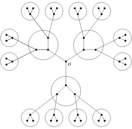
Figure 1: Partitioning the vertices ofT2 into families.
5.2 Proof of Theorem 1.3
For simplicity we will do the promised coupling onG=T2; the general case is analogous. Thus 1/r and 2/(1 +r) are now 1/2 and 2/3 respectively. Fix p “slightly” larger than 2/3, (where the “slightly” will be specified below) and let β =−log(1−p)/2 be the corresponding inverse temperature for the Ising model and note that by Lemma 5.3 we have thatµβ+6=µβ−. Fix a vertex o ∈ V. Couple X1, X2 ∈ {−1,1}V, where Xi is distributed according to µβi, in the following
way: First pick ( ˆX1(o),Xˆ2(o)) with the correct marginals in such a way that ˆX1(o)≤Xˆ2(o) and independently of all other vertices. Next partition V \ {o} into families, where each family is formed by one vertex at odd distance fromo(called the mother) together with the two neighbors of that vertex that are one step further away fromo(called the daughters). See Figure 1 for an illustration.
Note how this in a natural way gives rise to a “super-tree” where every “vertex” (i.e. family) but o has degree 5. Now order the families and define the coupling recursively: At each step pick the first family in the ordering for which the coupling has not yet been specified and which is connected to a family for which the coupling has been specified. Denote the vertices in this family m, d1 and d2; mother, daughter 1 and daughter 2 respectively. Let m0 be the “grand-mother”, i.e. the neighbor ofmwhich is notd1 ord2. If ˆX1(m0) = ˆX2(m0) then no disagreement percolation is possible through this family, so define the coupling in any way you like only so that ˆX1(m, d1, d2) ≤ Xˆ2(m, d1, d2) and independently of all other families. Assume now that
ˆ
Outcome Xˆ1(m, d1, d2) Xˆ2(m, d1, d2)
The only case for which there is a path of disagreements through the family is wheny=−x= (1,1,1) and this case gives rise to four new families in the “super-tree” through which disagree-ment percolation can continue. Thus the expected number of such families is 4·8/64 = 1/2<1 so that basic branching process theory tells us that the process of disagreement percolation will a.s. die out.
However, this is what would have been had p been exactly 2/3. On the other hand, by facts noted above, we can by letting p be larger than but close enough to 2/3 arrange things so that none of the conditional probabilities above changes by more than, say, 1/48 no matter what earlier couplings of other families have revealed so far. Then the above coupling does not have to be changed by more than so that the outcome ( ˆX1(m, d1, d2),Xˆ2(m, d1, d2)) = ((−1,−1,−1),(1,1,1)) gets an extra probability mass of 6/48. Thus the expected number of new families through which disagreement percolation can continue is bounded by 4(8/64 + 6/48) = 3/4<1 and we are still safe. This completes the desired coupling. ✷
Acknowledgment. I am grateful to Olle H¨aggstr¨om for inspiration and valuable discussions.
References
[1] I. Benjamini, R. Lyons, Y. Peres and O. Schramm, Group-invariant percolation on graphs,
[2] I. Benjamini and O. Schramm, Percolation beyond Z
d
, many questions and a few answers,
Electr. Comm. Probab. 1(1996), 71-82.
[3] J. van den Berg, A uniqueness condition for Gibbs measures, with application to the 2-dimensional Ising antiferromagnet,Commun. Math. Phys.152(1993), 61-66.
[4] J. van den Berg and C. Maes, Disagreement percolation in the study of Markov fields,Ann. Probab. 22(1994), 749-763.
[5] R. Grigorchuk and P. de la Harpe, Limit behaviour of exponential growth rates for finitely generated groups, Preprint 1999,
http://www.unige.ch/math/biblio/preprint/pp99.html.
[6] O. H¨aggstr¨om, A note on disagreement percolation,Random Struct. Alg. 18(2001), 267-278.
[7] O. H¨aggstr¨om, The random-cluster model on a homogeneous tree,Probab. Th. Rel. Fields104
(1996), 231-253.
[8] O. H¨aggstr¨om, J. Jonasson and R. Lyons, Explicit isoperimetric constants and phase tran-sitions in the random-cluster model,Annals of Probability, to appear,
http://www.math.chalmers.se/∼jonasson/recent.html.
[9] O. H¨aggstr¨om, Y.Peres and J. Steif, Dynamical percolation,Ann. Inst. H. Poincar´e, Probab. Statist.33 (1997), 497-528.
[10] J. Jonasson, The random cluster model on a general graph and a phase transition characteriza-tion of nonamenability,Stoch. Proc. Appl.79(1999), 335-354.
[11] H. Kesten, “Percolation Theory for Mathematicians, ” Birkh¨auser, Boston, 1982.
[12] J. C. Wierman, Bond percolation on honeycomb and triangular lattices, Adv. Appl. Prob. 13