23 11
Article 07.7.1
Journal of Integer Sequences, Vol. 10 (2007), 2
3 6 1 47
On the Behavior of a Variant of
Hofstadter’s Q-Sequence
B. Balamohan, A. Kuznetsov and Stephen Tanny
1Department of Mathematics
University Of Toronto
Toronto, Ontario M5S 2E4
Canada
[email protected]
Abstract
We completely solve the meta-Fibonacci recursion
V(n) =V(n−V(n−1)) +V(n−V(n−4)),
a variant of Hofstadter’s meta-FibonacciQ-sequence. For the initial conditionsV(1) = V(2) = V(3) = V(4) = 1 we prove that the sequence V(n) is monotone, with suc-cessive terms increasing by 0 or 1, so the sequence hits every positive integer. We demonstrate certain special structural properties and fascinating periodicities of the associated frequency sequence (the number of times V(n) hits each positive integer) that make possible an iterative computation ofV(n) for any value of n. Further, we derive a natural partition of theV-sequence into blocks of consecutive terms (“ genera-tions”) with the property that terms in one block determine the terms in the next. We conclude by examining all the other sets of four initial conditions for which this meta-Fibonacci recursion has a solution; we prove that in each case the resulting sequence is essentially the same as the one with initial conditions all ones.
1
Introduction
Hofstadter [7] introduced several integer sequences by self-referencing recurrences, including his now-famous Q-sequence defined as
with initial conditions Q(1) = Q(2) = 1. Virtually nothing has been proved about the enigmatic behavior of this sequence (see Table1and Figure1), including whether or not the sequence remains well defined for all positiven.2
Around 1999 Hofstadter and Huber [8] introduced the following family of sequences
Qr,s(n): for arbitrary positive integersr and s, with r<s,
Qr,s(n) = Qr,s(n−Qr,s(n−r)) +Qr,s(n−Qr,s(n−s)), n > s. (2)
They explored extensively the behavior of (2) for a wide range of (r, s) values and for various sets of initial conditions (Qr,s(1), Qr,s(2),. . . ,Qr,s(s)). Among their outstanding conjectures
from this largely empirical work is that for the initial values all ones the only values of (r, s) for which the recurrence (2) does not eventually become undefined (“dies”) are (1,2), (1,4) and (2,4).
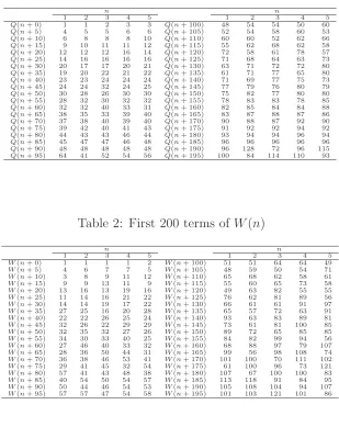
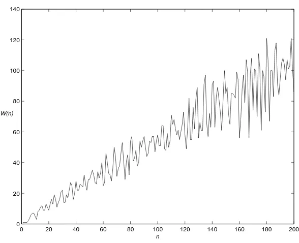
Notice that the case (r, s) = (1,2) is Hofstadter’s originalQ-sequence (which in the course of their latest work Hofstadter and Huber renamed the U-sequence). For (r, s) = (2,4), the sequence Q2,4(n) (renamed W(n)) appears to display even more inscrutably wild behavior;
compare Table 2 and Figure 2 to Table 1 and Figure 1, respectively. Like the original
Q-sequence, to date nothing has been proved about this sequence.
The focus of this paper is on the remaining case, where (r, s) = (1,4). In Table 3 we provide the first 200 values of the sequence Q1,4(n), which Hofstadter and Huber renamed
V(n). That is, in the following by V(n) we mean
V(n) =V(n−V(n−1)) +V(n−V(n−4)), n >4 (3)
and initial conditions V(1) =V(2) =V(3) =V(4) = 1.3
Despite its apparent simplicity, theV-sequence has many interesting properties.4 We
be-gin in Section2by proving that, like the Conolly and Conway meta-Fibonacci sequences (see [1, 9, 10]),V(n) is monotone increasing and successive terms differ by at most 1. However, in contrast to its better known cousins, V(n) never hits any number (other than 1) more than 3 times. We also estimate some bounds for V(n) and provide initial results relating to a generational structure for theV-sequence that we explore more fully in Section 4.
Evidently the V-sequence is determined by its frequency sequence, namely, the number of times thatV(n) hits each positive integer. In Section3we derive a precise understanding of the behavior of the frequency sequence. As a result, we are able to prove three recursive rules for generating the frequency sequence first conjectured by Gutman [8]. We conclude this section by noting some interesting patterns that occur in the frequency sequence.
Many meta-Fibonacci sequences, including the Conolly and Conway sequences with which
V(n) shares some properties, can be partitioned naturally into successive finite blocks of consecutive terms with common characteristics. In Section 4 we define such a partition for the V(n) sequence. Each term of V(n) in the kth block (suggestively called the “kth
2
That is, whether or notQ(n−1) andQ(n−2) are both less thannfor all positiven. If this is not the case we say the sequence “dies”. In a private communication Hofstadter indicates that theQ-sequence has been computed to billions of terms. On this basis it seems highly unlikely that the sequence dies.
3
Note thatV(n) appears in [13] as “SequenceA063882” where it is calledv(n).
4
0 20 40 60 80 100 120 140 160 180 200 0
20 40 60 80 100 120 140
n Q(n)
Figure 1: Graph of first 200 values of Hofstadter’s Q(n)
0 20 40 60 80 100 120 140 160 180 200
0 20 40 60 80 100 120 140
n W(n)
generation”) of this partition is a sum of two earlier terms, the first of which is in the (k−1)th block (generation) of the sequence. We provide general formulas for the starting
and ending indices for each block, and we deduce some periodicity properties concerning the frequencies of the sequence values at these starting and ending indices.
In Section 5 we examine all the sequences that result from (3) together with different sets of four initial conditions. We prove that there are only eight sets of initial conditions that generate a sequence that does not die. Each of the resulting sequences are essentially slightly truncated versions of the original V-sequence (with initial conditions all 1s).
We provide brief concluding remarks in Section 6.
2
Monotonicity
We begin by showing that the V-sequence is nondecreasing and hits every positive integer (other than 1) no more than 3 times.5 More precisely we show
Theorem 1. For V(n) defined in (3) above, the following holds
V(n)−V(n−1)∈ {0,1} f or n >1 (4)
V(n)−V(n−3)∈ {1,2} f or n >8 (5)
Proof. As in earlier work on meta-Fibonacci sequences (see, for example, [1, 6, 14]) it is
necessary to use a multi-statement induction proof on both (4) and (5) simultaneously. From Table3 (4) is true for n≤20 while (5) holds for 9≤n ≤20.
For the induction step we assume that (4) is true for all i < n and (5) is true for all 9≤ i < n where n > 20. We proceed to prove that these statements hold forn. We begin with (4).
By the definition (3) ofV we have
V(n)−V(n−1) = V(n−V(n−1)) +V(n−V(n−4)) (6)
−V(n−1−V(n−2))−V(n−1−V(n−5))
For ease of reference we adopt some suggestive “family-related” terminology.6 We say that
the term V(n) in “spot” n (the index of the term) is the child of the two V-sequence summands defined by the recursion (3), namely its mother V(n−V(n−1)) in spot (n−
V(n−1)) and its father V(n−V(n−4)) in spot (n−V(n−4)).
By the induction hypothesis on (4) we have V(n−1)−V(n−2) ∈ {0,1} and V(n−
4)−V(n−5)∈ {0,1}. Thus, in (6) , the difference between the mother spots ofV(n) and
V(n−1), that is, (n−V(n−1))−(n−1−V(n−2)) = 1−(V(n−1)−V(n−2)) is also
5
This result was first observed in 1999 by Hofstadter and Huber [8]. They have never published the details of their proof, which, according to Huber, is “a long, tedious, case by case tracking down of many branches of cases and sub-cases” involving the application of something he called “K-tables” (after Kellie Gutman).
6
0 or 1. By a similar argument we also have that the difference between the father spots of
V(n) and V(n−1), that is, (n−V(n−4))−(n−1−V(n−5)) = 1−(V(n−4)−V(n−5)), is also 0 or 1.
Suppose that V(n−1)−V(n−2) = 1. Then V(n−V(n−1)) = V(n−1−V(n−2)) and so the difference V(n)−V(n−1) in (6) is determined by the difference V(n−V(n−
4))−V(n−1−V(n−5)) of the fathers ofV(n) and V(n−1).
But since the difference between the fathers’ spots is 0 or 1, it follows from the induction hypothesis the difference between the fathers ofV(n) and V(n−1) is also 0 or 1 . Therefore statement (1) holds.
Similarly if V(n−4)−V(n−5) = 1 then V(n−V(n−4)) =V(n−1−V(n−5)) and (1) holds.
The only other case is both V(n−1)−V(n−2) = 0 andV(n−4)−V(n−5) = 0. Then the father spots (respectively, the mother spots) of V(n) and V(n−1) differ by 1.
Observe that if V(n − V(n −1)) = V(n −1 −V(n − 2)) then V(n)− V(n −1) =
V(n −V(n − 4))− V(n −1 −V(n −5)) ∈ {0,1}, as desired. So we may assume that
V(n−V(n−1)) =V(n−1−V(n−2)) + 1. Thus, besides the induction hypothesis we have the following set of assumptions:
V(n−1) = V(n−2) (7)
V(n−4) = V(n−5) (8)
V(n−V(n−1)) =V(n−1−V(n−2)) + 1 (9)
We now show that under all of the above assumptions we must have V(n −V(n −4)) =
V(n−1−V(n−5)), from which it follows by (6) that V(n)−V(n−1) = 1 and (1) holds for n.
By the induction hypothesis for (5)V(n−1)−V(n−4)∈ {1,2}. ButV(n−1) =V(n−2) soV(n−2)−V(n−4)∈ {1,2}. We have to consider two cases, namely,V(n−2) = V(n−4)+2 and V(n−2) = V(n−4) + 1.
Case 1: V(n−2) =V(n−4) + 2. This together with (7) means that (9) becomes
V(n−2−V(n−4)) =V(n−3−V(n−4)) + 1. (10)
Since V(n−2) = V(n−4) + 2 we must have V(n−2) = V(n−3) + 1 and V(n−3) =
V(n−4) + 1. But by the definition of theV functionV(n−2) = V(n−3) + 1 is equivalent toV(n−2−V(n−3)) +V(n−2−V(n−6)) =V(n−3−V(n−4)) +V(n−3−V(n−7)) + 1. Since V(n−3) = V(n−4) + 1, V(n−2−V(n −3)) = V(n−2−(V(n−4) + 1)) =
V(n−3−V(n−4)). Therefore
V(n−2−V(n−6)) =V(n−3−V(n−7)) + 1. (11)
Consequently we must have V(n−6) = V(n−7). But then since V(n−6) = V(n−7) and
V(n−5) = V(n−6)+1. Considering the last equation and the fact thatV(n−4) = V(n−5) (by (8) again), equation (11) can be rewritten as:
V(n−1−V(n−4)) =V(n−2−V(n−4)) + 1. (12)
From (10) and (12) we conclude thatV(n−1−V(n−4))−V(n−3−V(n−4)) = 2. But the induction hypothesis for (5) impliesV(n−V(n−4))−V(n−3−V(n−4)) ∈ {1,2}. Therefore, by (8) and the induction assumption on (4) we haveV(n−V(n−4)) =V(n−1−V(n−4)) =
V(n−1−V(n−5)). This completes the proof of Case 1.
Case 2: V(n−2) =V(n−4) + 1. By (7) and the definition of V(n) we can rewrite this as:
V(n−1−V(n−2)) +V(n−1−V(n−5)) (13) =V(n−4−V(n−5)) +V(n−4−V(n−8)) + 1.
But (7) and (8) also imply that V(n−1) = V(n−2) =V(n−5) + 1. Rewrite (9) as
V(n−1−V(n−5)) =V(n−2−V(n−5)) + 1. (14)
Substituting (14) into (13) we get
V(n−1−V(n−2)) +V(n−2−V(n−5)) (15) =V(n−4−V(n−5)) +V(n−4−V(n−8)).
Equivalently:
V(n−2−V(n−5))−V(n−4−V(n−8)) (16) =V(n−4−V(n−5))−V(n−2−V(n−5)).
But by the induction assumption for (5) we have V(n −5)− V(n −8) ∈ {1,2}. Thus
V(n−2−V(n−5))−V(n−4−V(n−8))≥0. At the same time, the induction assumption for (4) means thatV(n−4−V(n−5))−V(n−2−V(n−5))≤0. Hence both sides of(16) equal 0.
V(n−2−V(n−5))−V(n−4−V(n−5)) = 0. (17)
But (17) and the induction hypotheses (4) and (5) imply
V(n−4−V(n−5))−V(n−5−V(n−5)) = 1. (18)
Letk =n−V(n−5). Then by (3)
V(k)−V(k−1) = V(k−V(k−1)) +V(k−V(k−4)) (19)
−V(k−1−V(k−2))−V(k−1−V(k−5)).
Equation (14) is equivalent to V(k − 1) = V(k −2) + 1 and equation (18) implies that
We complete the induction by showing that (5) also holds forn. Observe the identity
V(n)−V(n−3) = (V(n)−V(n−1)) + (V(n−1)−V(n−3)). (20)
From what we have just proved, V(n)−V(n−1) is 0 or 1. Clearly V(n−1)−V(n−3) ∈ {0, 1, 2}by the induction assumption for (4). We consider three cases.
Case 1: V(n−1)−V(n−3) = 1. Then V(n)−V(n−3) is 1 or 2, by (20) and the fact that V(n)−V(n−1) is 0 or 1.
Case 2: V(n−1)−V(n−3) = 2. We show thatV(n) = V(n−1). WriteV(n−1)−V(n−
3) = (V(n−1)−V(n−2)) + (V(n−2)−V(n−3)). By the induction hypothesis for (4) each of the differences on the right-hand side is either 0 or 1. ThusV(n−1) =V(n−3) + 2 implies that V(n−1) =V(n−2) + 1 and V(n−2) =V(n−3) + 1. But by the induction hypothesis on (5) we have V(n−1)−V(n−4)∈ {1,2}, so V(n−4) =V(n−3).
Using the above relationships together with (3) we have
1 = V(n−1)−V(n−2)
= V(n−1−V(n−2)) +V(n−1−V(n−5))−V(n−2−V(n−3))
−V(n−2−V(n−6))
= V(n−1−V(n−5))−V(n−2−V(n−6)).
Therefore V(n−5) = V(n−6). Since V(n−4) = V(n−3) the induction assumption on (4) and (5) implies that V(n−4) =V(n−5) + 1. Again, by (3),
V(n)−V(n−1) = V(n−V(n−1)) +V(n−V(n−4))
−V(n−1−V(n−2))−V(n−1−V(n−5))
SubstitutingV(n−1) =V(n−2) + 1 and V(n−4) =V(n−5) + 1 into the above equation we get the desired result V(n)−V(n−1) = 0.
Case 3: V(n−1)−V(n−3) = 0. We show that V(n) = V(n−1) + 1, which together with (20) completes this case and the proof of (5). By (3) we have
V(n)−V(n−3) = V(n−V(n−1)) +V(n−V(n−4)) (21)
−V(n−3−V(n−4))−V(n−3−V(n−7)).
SinceV(n−1)−V(n−3) = 0 by the induction hypothesis on (5) we must haveV(n−3)−
V(n−4) = 1. Using these two relations we rewrite (21) as
V(n)−V(n−3) = V(n−1−V(n−4)) +V(n−V(n−4))
−V(n−3−V(n−4))−V(n−3−V(n−7)).
By the induction hypothesis for (5) we have thatV(n−V(n−4))−V(n−3−V(n−4)) ∈ {1,2}, whileV(n−V(n−1)) =V(n−V(n−3)) =V(n−1−V(n−4))≥V(n−3−V(n−7)). (To see the last inequality, observe that by the induction on (5) we haveV(n−4)−V(n−7)∈ {1,2}. Thus, eitherV(n−1−V(n−4)) =V(n−2−V(n−7)), in which case we know the inequality by monotonicity, orV(n−1−V(n−4)) =V(n−3−V(n−7)), in which case the two terms are identical and the difference is 0.) ThusV(n)−V(n−3)>0, and therefore we must have
We now prove several relationships between the mother and father spots. These simple results provide some essential tools for establishing our main findings in the following section.
Corollary 2. Suppose the mother spot of V(n) ism and the father spot ofV(n)isf. Then:
(i) the mother spot of V(n+ 1) ism if V(n) =V(n−1) + 1 and m+ 1 otherwise;
(ii) the father spot of V(n+ 1) isf if V(n−3) =V(n−4) + 1 and f+ 1 otherwise.
Proof. Recall from the proof of Theorem 1 that the difference in the mother (respectively,
father) spots for the two consecutive indices n and n + 1 is 1−(V(n)−V(n −1)) and (1−(V(n−3)−V(n−4))) . The corollary now follows immediately from the results of Theorem 1.
Remark: It follows immediately from Corollary 2 and Theorem 1that there is a natural definition for the sequences of the mother spot and the father spot, respectively, and for the mother and father sequences. All these sequences are monotonic increasing, and have successive differences that are either 0 or 1.
Corollary 3. Suppose that the mother spot of V(n) is m. Then the father spot of V(n) is
m+ 1 if V(n−1) =V(n−4) + 1 and m+ 2 if V(n−1) =V(n−4) + 2.
Proof. The proof is analogous to the preceding result. By definition, the mother and father
spots of V(n) are n−V(n−1) and n−V(n−4) respectively. If V(n−1) =V(n−4) + 1 then father spot of V(n) is n−V(n−4) =n−(V(n−1)−1) = n+ 1−V(n−1) =m+ 1. By Theorem 1 the only other possible situation is V(n−1) = V(n−4) + 2, in which case the father spot ofV(n) isn−V(n−4) =n−(V(n−1)−2) = n+ 2−V(n−1) =m+ 2.
Corollary 4. The father and mother of V(n) differ by 0, 1 or 2. More precisely, V(n−
V(n−4))−V(n−V(n−1)) ∈ {0,1,2}.
Proof. By Corollary3 the father spot f and mother spot m differ by 1 or 2. If f =m+ 1,
then V(f)−V(m)∈ {0,1}, while if f =m+ 2, thenV(f)−V(m) = (V(f)−V(f −1)) + (V(f−1)−V(m))∈ {0,1,2}.
We conclude this section with an estimate for the size ofV(n).
Proposition 5. For all n >6, we have n
2 < V(n)≤
n
2 + log2n−1.
Proof. We prove both these bounds by induction. We start with the lower bound. The base
case is evident from Table 3for many small values of n > 6. Assume it holds up to K >6. ForK+ 1 we have the following inequalities: V(K+ 1)≥2V(K+ 1−V(K)) (by Theorem
1) > K+ 1−V(K) (by the induction assumption) ≥ K + 1−V(K + 1) (by Theorem 1). The required result now follows.
For the upper bound, we proceed as follows. Let V(n) = a, where a > 1. Note that
a < n. We show an even stronger result, namely,V(n) = a≤ n
where A ≥ 5, and let V(n) =A. Then A = V(n) = V(n−V(n−1)) +V(n−V(n−4)). Applying the induction hypothesis to the terms on the right-hand side we get
V(n) ≤ (n−V(n−1))/2 + log2(V(n−V(n−1)) + (n−V(n−4))/2 + log2(V(n−V(n−4))−2 in the last of the above inequalities, we get
V(n)≤ n−V(n) + 1
Since V(n) is an integer the following corollary is immediate.
Corollary 6. For all n >6, ⌈n We have found empirically that the midpointP(n) of the interval defined by the bounds in Corollary6provides a very good estimate for the value of V(n). We empirically determined the error
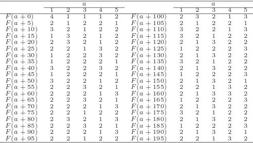
The behavior of V(n) is completely determined by the frequency with which it hits each positive integer.7 For any positive integer a, let F(a) (the “frequency” of a) denote the
number of occurrences of a in the sequence V(n). By Theorem 1, for a > 1, we have 1≤F(a)≤3. Table 4shows the first 200 values of the frequency sequence.
The frequency sequence exhibits many interesting “local” properties (see Lemmas 9-12
below). For example, no two consecutive 1s appear, and there are never more than three consecutive 2s. The pair 12 is always followed by a 2. No more than two consecutive 3s occur, and indeed, such occurrences of consecutive 3s in the frequency sequence are relatively rare.
7
Table 4: First 200 values of frequency sequence F(a) of V(n)
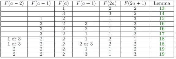
The frequency sequence also exhibits the following “remote” characteristic: for any pos-itive integer a the frequencies with which 2a and 2a+ 1 occur depend upon the frequency of a in certain cases, and of a and some of its neighbors (a−2,a−1, and a+ 1) in others (see Lemmas13-19). We refer to this as the “index doubling” property. The index doubling results, which are summarized in Table5, are key to proving a set of three rules first observed by Gutman [4] for generating the frequency sequence of V(n) recursively. We conclude this section by describing some additional properties of the frequency sequence that follow from Table 5.
The following assertions are all for a ≥ 6 and for n ≥ 21. We begin with two technical results on the size of the mother and father values for even and odd values of theV-sequence.
Lemma 7. Suppose that for some positive integer a V(n) = 2a. Then:
(i) the mother and father are both equal to a, which occurs if and only if F(a)>1;
(ii) the mother is equal to a−1 and the father is equal to a+ 1, which occurs if and only
if F(a) = 1.
Proof. By Corollary 4 the father and mother of V(n) differ by 0, 1 or 2. Since V(n) = 2a
the mother and father cannot differ by 1. Thus either both the mother and father are equal toa, or they differ by 2, so that the mother is equal to a−1 and father is equal to a+ 1.
By Corollary3the mother and father spots always differ by 1 or 2. It follows that if both the mother and father ofnare equal toa, thenF(a)>1. Conversely, supposeF(a)>1. By Corollary 3 the difference between the father spot and the mother spot is at most 2. Since
F(a) >1 it follows (since the V-sequence is monotonic with successive differences either 0 or 1) that the mother and father can differ by at most 1. But we have already observed that when V(n) = 2a the mother and father cannot differ by 1. Thus the mother and father of
V(n) are both equal to a. This proves (i).
In the second case, if the mother is equal to a−1 and the father is equal to a+ 1, then
Lemma 8. If V(n) = 2a+ 1for some positive integera, then mother and father are
respec-tively a and a+ 1.
Proof. By Corollary 4 the mother and father differ by 0, 1 or 2. If their difference is 0 or
2 then their sum is an even number. So their difference must be 1. Thus the mother and father area and a+ 1, respectively.
We now prove some local properties of theV-sequence.
Lemma 9. Suppose F(a) = 1. Then F(a+ 1) >1.
Proof. Let m be the maximum of {i : V(i) = a −1} and suppose F(a + 1) = 1. Then
V(m+ 1) = a, V(m+ 2) = a+ 1 and V(m+ 3) = a+ 2. So V(m+ 3)−V(m) = 3. This contradicts Theorem1. Therefore F(a+ 1)>1.
An immediate consequence of Lemma 9, first observed by Huber [8], is that V(n) does not have a string of four consecutive strictly increasing terms.
Lemma 10. SupposeF(a) = 1. Then F(a+ 2) >1 and F(a−1) = 2.
Proof. Let n be the unique index such that V(n) = a. Applying Lemma 9 (twice) and
Theorem 1 we deduce that there are the following two possibilities:
(i) V(n −2) = V(n −1) = a −1, V(n) = a, V(n + 1) = a + 1, V(n+ 2) = a+ 1,
V(n+ 3) =a+ 2;
(ii) V(n −2) = V(n −1) = a −1, V(n) = a, V(n + 1) = a + 1, V(n+ 2) = a+ 1,
V(n+ 3) =a+ 1, V(n+ 4) =a+ 2.
In case (i), sinceV(n+ 3) =V(n+ 2) + 1 andV(n) = V(n−1) + 1,V(n+ 4) =V(n+ 4−
V(n+ 3)) +V(n+ 4−V(n)) =V(n+ 3−V(n+ 2)) +V(n+ 3−V(n−1)) =V(n+ 3) =a+ 2. Thus,F(a+ 2)>1, as required.
Now, by the definition of the V-sequence, V(n+ 1) =V(n) + 1 is equivalent toV(n+ 1−
V(n))+V(n+1−V(n−3)) =V(n−V(n−1))+V(n−V(n−4))+1. SinceV(n) =V(n−1)+1 we have V(n+ 1−V(n)) = V(n−V(n−1)). Hence
V(n+ 1−V(n−3)) =V(n−V(n−4)) + 1. (23)
Since successive terms of theV-sequence differ by 0 or 1 this means thatV(n−3) =V(n−4). But V(n−1) =V(n−2) = a−1 and since the frequency is always less than 4, Theorem 1
implies thatV(n−2) =V(n−3) + 1. Thus, F(a−1) = 2.
In case (ii), sinceV(n+ 4) =V(n+ 3) + 1 andV(n+ 1) =V(n) + 1, V(n+ 5) =V(n+ 5−
V(n+ 4)) +V(n+ 5−V(n+ 1)) =V(n+ 4−V(n+ 3)) +V(n+ 4−V(n)) =V(n+ 4) =a+ 2. Once again, F(a+ 2) > 1. The proof that F(a−1) = 2 in this case is identical to case (i).
Proof. The setup is the same as case (i) in Lemma 10, with the additional condition V(n+ 4) = a+ 2, which follows from Lemma 10. Thus V(n−3) = V(n−4) = V(n+ 3)−4 =
V(n+ 4)−4. We use these last equations to rewrite (23) as follows:
V(n+ 5−V(n+ 4)) =V(n+ 4−V(n+ 3)) + 1 (24)
But (24) is precisely the difference between mothers of V(n + 5) and V(n + 4). Hence
V(n+ 5) =V(n+ 4) + 1 andF(a+ 2) = 2.
Lemma 12.
(i) If F(a) =F(a+ 1) =F(a+ 2) = 2 then F(a+ 3)6= 2. (ii) If F(a−1) =F(a−2) = 3, then F(a) = 2.
Proof. (i) Letn be the minimum of{i:V(i) =a+ 3}. From the given frequencies we have
V(n−1) =V(n−2) =a+ 2, V(n−3) = V(n−4) =a+ 1, and V(n−5) =V(n−6) = a. Assume thatF(a+ 3) = 2. ThenV(n) =V(n+ 1) =a+ 3 and V(n+ 2)−V(n+ 1) = 1. We show that this leads to a contradiction.
Let m be the mother spot of V(n). As in the preceding proofs we apply Corollaries 2
and 3 to deduce each of the following in turn:
V(n) = V(m) +V(m+ 1)
V(n+ 1) =V(m) +V(m+ 2)
V(n+ 2) =V(m+ 1) +V(m+ 2)
V(n−1) = V(m−1) +V(m+ 1)
V(n−2) = V(m−1) +V(m)
From the above relations we have V(n+ 2)−V(n+ 1) =V(m+ 1)−V(m) =V(n−1)−
V(n−2) = 0, a contradiction. Thus F(a+ 3)6= 2.
(ii)Letnbe the minimum of{i: V(i) = a}. ThenV(n−1) =V(n−2) =V(n−3) =a−1 and V(n−4) = V(n−5) =V(n−6) = a−2.
By definition, V(n+ 1)−V(n) =V(n+ 1−V(n)) +V(n+ 1−V(n−3))−V(n−V(n−
1))−V(n−V(n −4)). But since V(n) = V(n−1) + 1 and V(n−3) = V(n−4) + 1 it follows thatV(n+ 1) =V(n).
Similarly we have V(n+ 2)−V(n+ 1) =V(n+ 2−V(n+ 1)) +V(n+ 2−V(n−2))−
V(n+ 1 −V(n))−V(n+ 1 −V(n−3)). But V(n + 1) = V(n) = V(n −3) + 1 so the first and last terms of this expression cancel and we are left with V(n+ 2)−V(n+ 1) =
V(n+ 2−V(n−2))−V(n+ 1−V(n)). Further, since V(n) =V(n−2) + 1 we also have that V(n+ 2)−V(n+ 1) =V(n+ 3−V(n))−V(n+ 1−V(n)).
In the same way, using (3) and the fact that V(n−2) = V(n−6) + 1, we derive that
V(n−1)−V(n−2) =V(n−1−V(n−5))−V(n−2−V(n−3)). ButV(n−1) =V(n−2) soV(n−1−V(n−5)) =V(n−2−V(n−3)). But sinceV(n−5) =V(n−3)−1 =V(n)−2 this means thatV(n+ 1−V(n)) =V(n−1−V(n)). Thus we haveV(n+ 2)−V(n+ 1) =
Lemma 12 completes our focus on the local properties of the frequency sequence. We now show how the frequency of a and some of its neighbors determine the frequency of 2a and 2a+ 1. Once this is done, we have an implicit algorithm to determine any value in the frequency sequence, and hence we understand precisely the behavior of the original
V-sequence.
Lemma 13. If F(a) = 1 then F(2a) =F(2a+ 1) = 2.
Proof. Let n be the minimum of {i : V(i) = 2a} and m be the unique index such that
V(m) = a. By Lemma 7, together with the fact that the V-sequence is monotonic with successive differences either 0 or 1, it follows thatV(n) =V(m−1) +V(m+ 1).
By the definition of n, we have V(n) = V(n−1) + 1. By definition, the mother spot of
V(n) is m−1, so by Corollary 2the mother spot of V(n+ 1) is alsom−1. Since the father spot of V(n) is m+ 1, it follows from Corollary 2 that the father spot ofV(n+ 1) is either
m+ 1 or m+ 2. But by Corollary 3, the father spot must be m+ 1 since the mother and father spot differ by at most 2. Thus, V(n+ 1) =V(n) = 2a, so F(2a) is at least 2.
Again, by Corollary 2 the mother spot ofV(n+ 2) must bem. By Corollary 3we must haveV(n+ 2) =V(m) +V(m+ 1) orV(n+ 2) =V(m) +V(m+ 2). HenceV(n+ 2) = 2a+ 1 since by Lemma 9 V(m+ 1) =V(m+ 2) =a+ 1. Thus F(2a) = 2.
The argument to show thatF(2a+ 1) = 2 is similar. By Corollary2 the mother spot of
V(n+ 3) ism. Hence V(n+ 3) = V(m) +V(m+ 1) orV(n+ 3) =V(m) +V(m+ 2). Since
V(m+ 1) =V(m+ 2) we have V(n+ 3) =V(n+ 2) = 2a+ 1 and F(2a+ 1) is at least 2. Once again by Corollary2the mother spot ofV(n+4) ism+1. ButV(m+1) =V(m)+1, thusV(n+ 4)> V(n+ 3) and so F(2a+ 1) = 2 as desired.
Lemma 14. If F(a) = 3 then F(2a) = 3 and F(2a+ 1) = 2.
Proof. Let n, m be the minimum of {i: V(i) = 2a} and {j :V(j) =a} respectively. Since
F(a)>1, by Lemma 7we must have that both the mother and father ofV(n) are equal to
a. Since F(a) = 3 then by Corollary 3 we know that either V(n) = V(m) +V(m+ 1) or
V(n) = V(m) +V(m+ 2).
By Corollary 2the mother spot of V(n+ 1) is m. Thus V(n+ 1) =V(m) +V(m+ 1) or
V(n+ 1) =V(m) +V(m+ 2). Hence V(n+ 1) =V(n) = 2a since F(a) = 3.
Similarly, by Corollary 2, the mother spot of V(n+ 2) is m + 1. Thus V(n + 2) =
V(m+ 1) +V(m+ 2) orV(n+ 2) =V(m+ 1) +V(m+ 3). IfV(n+ 2) =V(m+ 1) +V(m+ 2) then V(n+ 2) = 2a.
If V(n+ 2) =V(m+ 1) +V(m+ 3) then the father spot of V(n+ 2) is two more than the mother spot. That is, (n+ 2−V(n−2)) = (n+ 2−V(n+ 1)) + 2. This is equivalent toV(n−2) =V(n+ 1)−2 = 2a−2.
Now V(n−1)≥2V(n−1−V(n−2)) as the mother is always less than or equal to the father. That is,V(n−1)≥2V(n−1−(2a−2)) = 2V(n+1−2a). Butn+1−2ais the mother spot ofV(n+ 1), so we haveV(n−1)≥2V(m) = 2a. But this contradicts the definition of
n as the minimum of {i : V(i) = 2a}. Thus V(n+ 2) = V(m+ 1) +V(m+ 2) = 2a, and
By Corollaries 2and 3, we can compute the following values:
V(n+ 3) =V(m+ 2) +V(m+ 3) = 2a+ 1
V(n+ 4) =V(m+ 2) +V(m+ 3) = 2a+ 1
V(n+ 5) =V(m+ 3) +V(m+ 4)≥2V(m+ 3) = 2a+ 2
This shows thatF(2a+ 1) = 2, and completes the proof.
Lemma 15. If F(a−1) = 1 and F(a) = 2 then F(2a) = 1 and F(2a+ 1) = 3.
Proof. Let n, m be the minimum of {i: V(i) = 2a} and {j :V(j) =a} respectively. Since
F(a−1) = 1, by Lemma13 F(2a−2) =F(2a−1) = 2. By the definition ofn this implies that V(n−1) =V(n−2) = 2a−1 and V(n−3) =V(n−4) = 2a−2.
Since F(a) = 2, V(m) = V(m+ 1) = a. Since V(n) = 2a it follows by Corollary 3 and Lemma7thatV(n) =V(m) +V(m+ 1). Then by Corollary2the mother spot ofV(n+ 1) is
m. By Corollary3, the father spot ofV(n+1) ism+2, sinceV(n)−V(n−3) = 2a−(2a−2) = 2. But F(a) = 2 so V(m+ 2) = a+ 1. Thus V(n+ 1) = V(m) +V(m+ 2) = 2a+ 1 so
F(2a) = 1.
In a similar way, we can show thatV(n+ 2) =V(m) +V(m+ 2) = 2a+ 1 andV(n+ 3) =
V(m+ 1) +V(m+ 3) = 2a+ 1, so F(2a+ 1) = 3.
Lemma 16. If F(a −1) = 3, F(a) = 2 and F(a + 1) = 3 or 2 then F(2a) = 1 and
F(2a+ 1) = 3.
Proof. Let n, m be the minimum of {i : V(i) = 2a} and {j : V(j) = a} respectively. By
Lemma14, V(n−1) =V(n−2) = 2a−1, and V(n−3) =V(n−4) = V(n−5) = 2a−2. By the now familiar argument, since F(a) >1, we deduce using Lemma 7 that V(n) =
V(m)+V(m+1) = 2a. Then by Corollary2we conclude thatV(n+1) =V(m)+V(m+2) = 2a+1. SimilarlyV(n+2) =V(m)+V(m+2) = 2a+1 andV(n+3) =V(m+1)+V(m+3) = 2a+ 1.
Lemma 17. IfF(a−1) = 3, F(a) = 2and F(a+ 1) = 1thenF(2a) = 1and F(2a+ 1) = 2.
Proof. Let n, m be the minimum of {i : V(i) = 2a} and {j : V(j) = a} respectively.
Since F(a−1) = 3 Lemma 14, together with the definition of n, implies that V(n−1) =
V(n−2) = 2a−1 and V(n−3) = V(n−4) = V(n−5) = 2a−2. Then by Lemma 7,
V(n) =V(m) +V(m+ 1) = 2a. Once again we conclude the proof by invoking Corollary 2
to deduce the following relations:
V(n+ 1) =V(m) +V(m+ 2) = 2a+ 1
V(n+ 2) =V(m) +V(m+ 2) = 2a+ 1
V(n+ 3) =V(m+ 1) +V(m+ 3) = 2a+ 2
Lemma 18. If F(a−2) 6= 2, and F(a −1) = F(a) = 2 then F(2a) = 2. Moreover, if
Proof. Letn, m be the minimum of {i:V(i) = 2a} and {j :V(j) =a} respectively. By the given conditions on the frequencies ofa−2,a−1 anda, we can apply Lemmas 15and16to deduce thatF(2a−2) = 1 and F(2a−1) = 3. Together with the definition of n this yields
V(n−4) = 2a−2 and V(n−3) =V(n−2) =V(n−1) = 2a−1. Then by Lemma 7 and Corollary3, V(n) = V(m) +V(m+ 1) = 2a. Now by Corollary2 we deduce
V(n+ 1) =V(m) +V(m+ 1) = 2a
V(n+ 2) =V(m+ 1) +V(m+ 2) = 2a+ 1
V(n+ 3) =V(m+ 1) +V(m+ 3).
IfF(a+1) = 1 thenV(n+3) =a+(a+2) = 2a+2 andF(2a+1) = 1. OtherwiseF(a+1) = 2 or 3 and then V(n+ 3) = 2a+ 1 while V(n+ 4) = V(m+ 2) +V(m+ 3) = 2a+ 2. Thus,
F(2a+ 1) = 2.
Lemma 19. IfF(a−2) =F(a−1) =F(a) = 2, thenF(2a) = 1. Furthermore ifF(a+1) = 1
then F(2a+ 1) = 2 and if F(a+ 1) = 3 then F(2a+ 1) = 3.
Proof. By Lemma12it follows thatF(a−3) = 3 or 1. By Lemmas15,16and18F(2a−4) =
1,F(2a−3) = 3, F(2a−2) = 2 and F(2a−1) = 2.
Let n, m be the minimum of {i : V(i) = 2a} and {j : V(j) = a} respectively. Then
V(n−1) =V(n−2) = 2a−1,V(n−3) =V(n−4) = 2a−2. By Corollary7 and Lemma
7,V(n) =V(m) +V(m+ 1) = 2a. Now by Corollary 2we have
V(n+ 1) =V(m) +V(m+ 2) = 2a+ 1
V(n+ 2) =V(m) +V(m+ 2) = 2a+ 1
V(n+ 3) =V(m+ 1) +V(m+ 3)
From these it follows that if F(a+ 1) = 1 then V(n+ 3) = 2a+ 2 so F(2a+ 1) = 2, while if
F(a+ 1) = 3 thenV(n+ 3) = 2a+ 1 and F(2a+ 1) = 3. This completes the proof.
Table 5: Frequencies of 2a and 2a + 1 in terms of the frequencies of a and some of its neighbors.
F(a−2) F(a−1) F(a) F(a+ 1) F(2a) F(2a+ 1) Lemma
1 2 2 13
3 3 2 14
1 2 1 3 15
3 2 3 1 3 16
3 2 2 1 3 16
3 2 1 1 2 17
1 or 3 2 2 1 2 1 18
1 or 3 2 2 2 or 3 2 2 18
2 2 2 1 1 2 19
2 2 2 3 1 3 19
the values of the frequency sequence iteratively. One natural way to do so is in successive intervals of length 2k for k >2.
We illustrate what we mean. From Table 4 the frequency sequence for a∈ [4,7] is 1, 2, 2, 1. It follows from Table 5that the values of the frequency sequence from 8 to 15 must be 2, 2 (13) 1, 3 (15) 2, 1 (18) 2, 2 (13), where we have put the lemma number from the last column in Table5 between consecutive pairs of frequency values to highlight how the table applies.
In a similar way we can fill in the values of the frequency sequence from 16 to 31, 32 to 63, 64 to 127, and so on. Note, however, that becauseF(2a) andF(2a+ 1) can depend upon the value of F(a−2),F(a−1) and F(a+ 1) it may be the case that the frequency values at the start and endpoints of an interval depend upon frequency values slightly outside the immediately preceding interval, either in the prior interval of length a power of 2 or in the current such interval. For example, F(30) and F(31) in [16,31] are determined by F(13),
F(14),F(15) andF(16);F(32) andF(33) in [32,63] are determined by F(14), F(15),F(16) and F(17).
In Table 6 we highlight the pattern in the frequencies at the start and endpoints of the intervals [2k,2k+1 - 1] for k = 2 through 11. Perhaps not unexpectedly, these frequencies are
periodic; that is, beginning with the interval starting at 64 and ending at 127, the frequencies for the start points for successive intervals are 1, 2, 2, 1, 2, 2,· · · while the frequencies for the endpoints for these same intervals are 2, 3, 2, 2, 3, 2,· · ·. This result follows directly from Table 5by induction.
Table 6: Values of the frequency sequence at the start and endpoints of the intervals [2k,2k+1−
1].
Start End F(Start) F(End)
4 7 1 1
8 15 2 2
16 31 1 1
32 63 2 2
64 127 1 2
128 255 2 3
256 511 2 2
512 1023 1 2
1024 2047 2 3
2048 4095 2 2
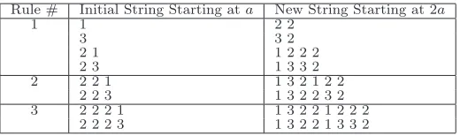
Gutman [8] identified (but never proved) a set of simply stated rules for recursively generating the frequency sequence ofV(n) (see Table7). These rules explain how the values of the frequency sequence starting at 2a can be derived from the values of the sequence starting ata. Rule 3 takes precedence over Rule 2, which in turn takes precedence over Rule 1.
Each of Gutman’s rules follow from Table 5 and the earlier lemmas. For example, the first part of Rule 1 is Lemma 13(note that Gutman has no rule covering the pair 11, which cannot occur by Lemma9). Lemma 12assures that there is no need for a rule covering four consecutive 2s. To derive the first part of Rule 3, namely that the string 2 2 2 1 generates the new string 1 3 2 2 1 2 2 2 in the next interval, argue as follows: apply Lemmas 15 and
Table 7: Gutman’s rules for generating the frequency sequence of V(n)
Rule # Initial String Starting ata New String Starting at 2a
1 1 2 2
3 3 2
2 1 1 2 2 2
2 3 1 3 3 2
2 2 2 1 1 3 2 1 2 2
2 2 3 1 3 2 2 3 2
3 2 2 2 1 1 3 2 2 1 2 2 2 2 2 2 3 1 3 2 2 1 3 3 2
we can justify all the other components of Gutman’s rules, and verify that they cover all possible cases.
We show below that taken together Gutman’s rules generate the frequency sequence. However, it is no longer the case that successive intervals beginning at powers of 2 are the natural division points in this process. That’s because the varying string lengths together with the precedence guidelines accompanying Gutman’s rules may require that we pass these division points in order to apply the appropriate rule. As a result we gradually drift further and further away from the powers of 2 as natural division points in generating the sequence using Gutman’s rules. For example, applying Gutman’s rules, [8, 16] are required to generate [16, 33]; [17, 34] are required to generate [34, 69]; [35-70] are required to generate [70, 141]; and so on.
To see that Gutman’s rules will generate the frequency sequence, it is probably best to begin at a term like F(11), which under her approach is a string of length 1 with value 3. This single 3 at 11 unambiguously becomes 3 2 at 22 and 23. Further, note that under Gutman’s rules the 3 at the end of any string necessarily becomes the pair 3 2 in the new string, no matter what string the initial 3 is contained in. Thus, the 3 at 22 necessarily leads to a 3 at 44, and so on. In this way there is no drift (since it is not necessary to know the values of the sequence following the 3) and a straightforward induction argument using Table5yields the desired result. (Note that this same argument holds for our rules in Table 5 as well.)
The frequency sequence has many other interesting properties, all of which can be proven using the results we have described above together with an induction argument.8 These
include
(P1) The 1s are natural markers of the frequency sequence, since no two consecutive 1s occur. There are precisely ten different strings of 2s and 3s that can occur between successive 1s, all of which end with 2.9
(P2) The value 3 occurs relatively less often in the frequency sequence. There are precisely ten different strings of 1s and 2s that can occur between successive 3s, including the empty string corresponding to the pair 3 3;
(P3) The string (3, 2, 2, 1, 3) always follows the string (3, 2, 1, 2, 2, 1, 3) (except for the first occurrence of the latter string beginning at 11). Note that the last 3 in (3, 2, 1,
8
The interested reader can contact us for an Appendix containing further details.
9
2, 2, 1, 3) also is the first 3 in (3, 2, 2, 1, 3);
(P4) Pairs of consecutive 3s occur very infrequently. There are 17 distinct strings of 1s, 2s and 3s that can occur between successive pairs of 3s. (Recall from Lemma12 that at most two consecutive 3s can occur; in fact, we can also show from Table5that the first 3 in any such pair of consecutive 3s occurs at an odd index of the frequency sequence.)
4
V-sequence Generational Structure
Many meta-Fibonacci sequences have been shown to have an underlying structure that leads to a natural partition of the sequence into successive finite blocks of consecutive entries (see, for example, [1, 9,10, 11, 12,14]). Following Pinn [11, 12] we suggestively call these blocks
“generations”. The basic idea for this partition is the observation that the terms of the
sequence that make up the kth block (generation) are defined by the original recursion as
sums of certain earlier terms in the sequence that come (at least in part - see below) from the (k−1)th generation.
In this way we build a family tree for the terms of the meta-Fibonacci sequence. This procedure is analogous to a well-known approach to understanding the pedigree of the terms in the usual Fibonacci sequence (see, for example, [3], chapter 6).
One such natural partition for the V-sequence is defined as follows10: for n > 4 define
the “maternal” sequence
M(n) = M(n−V(n−1)) + 1, with M(n) = 1f or n= 1, 2, 3, and4. (25)
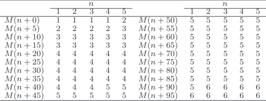
See Table8 for the first 100 values of M(n).
Notice that the value of M(n) is one more than the value of the M-sequence at the mother spot (n −V(n−1)) of V(n). In this sense we are considering V(n) as the “next generation” of its motherV(n−V(n−1)) who is a member of the previous generation with number M(n−V(n−1)).
This is the motivation for calling M(n) the maternal generation number of V(n). We say that G(k) = {n : M(n) = k} is the kth maternal generation of V(n).11 Notice that we
place no restriction on the pedigree of the father term V(n−V(n−4)).
A priori it is not evident thatM(n) necessarily induces a partition on theV(n) sequence that conforms to our intuition about the way a generational structure should operate. How-ever, we can easily show that this is the case.
Proposition 20. LetM(n)be defined as above. Then for all positive integersn, M(n+1) =
M(n) or M(n) + 1.
10
This approach, which can be substantially generalized, leads to a natural generation structure for a wide variety of meta-Fibonacci sequences. As such it may provide a unifying theme for certain similar types of meta-Fibonacci recursions, something which to date is sorely lacking. It will be the topic of a future communication. See [2] for some initial results.
11
Table 8: The first 100 values of M(n)
n n
1 2 3 4 5 1 2 3 4 5
M(n+ 0) 1 1 1 1 2 M(n+ 50) 5 5 5 5 5
M(n+ 5) 2 2 2 2 3 M(n+ 55) 5 5 5 5 5
M(n+ 10) 3 3 3 3 3 M(n+ 60) 5 5 5 5 5
M(n+ 15) 3 3 3 3 3 M(n+ 65) 5 5 5 5 5
M(n+ 20) 4 4 4 4 4 M(n+ 70) 5 5 5 5 5
M(n+ 25) 4 4 4 4 4 M(n+ 75) 5 5 5 5 5
M(n+ 30) 4 4 4 4 4 M(n+ 80) 5 5 5 5 5
M(n+ 35) 4 4 4 4 4 M(n+ 85) 5 5 5 5 5
M(n+ 40) 4 4 4 5 5 M(n+ 90) 5 6 6 6 6
M(n+ 45) 5 5 5 5 5 M(n+ 95) 6 6 6 6 6
Thus, M(n) is an increasing sequence with successive differences either 0 or 1, so that the kth generation of the V-sequence is the interval of consecutive values of n such that
M(n) = k. Hence the sets G(k) are non-empty disjoint intervals that partition the natural numbers. We call the starting index or start point (respectively, ending index orend point) of the kth generation G(k) the least (respectively, greatest) value of n such that M(n) = k.
Proof. We proceed by induction. By definition, M(1) = M(2) = M(3) = M(4) = 1 and
M(5) =M(5−V(4)) + 1 = M(4) + 1 = 2.
Assume the result up to k ≥ 4. Then M(k+ 1) = M(k+ 1−V(k)) + 1. Now V(k) =
V(k−1) or V(k−1) + 1. In the latter case, M(k+ 1) =M(k+ 1−(V(k−1) + 1)) + 1 =
M(k−V(k−1)) + 1 =M(k), as required.
IfV(k) = V(k−1), thenM(k+1) =M((k−V(k−1))+1)+1. Since (k−V(k−1))+1< k+ 1, we have by the induction assumption thatM((k−V(k−1)) + 1) =M(k−V(k−1)) or
M(k−V(k−1))+1. In the first case we conclude thatM(k+1) =M(k−V(k−1))+1 =M(k). In the second case we haveM(k+ 1) =M(k−V(k−1)) + 1 + 1 =M(k) + 1.12
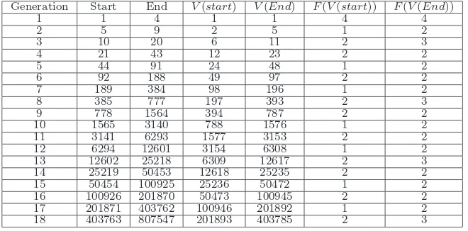
In Table9we illustrate the sets corresponding to the first 18 generations ofV(n), together with the associated frequencies of the start and endpoints of each generation.
The maternal generation concept is very appealing as a natural way to identify the generation structure for the V-sequence. From Table 9 it is evident that after generation 2 the length of successive maternal generations approximately doubles. This seems natural based on what we already know about the sequence from Sections 2and 3.
Further, as we prove below (see Proposition 22), the start point for each generation coincides with the first occurrence of a new V-sequence value while the end point of each generation marks the last occurrence of some V-sequence value. For example, we see from Tables 9 and 3 that generation 3 has start point (or begins) at 10, which is the index for the first 6 in the sequence (there are 2) and has end point (or ends) at index 20, where the
V-sequence value is the last of three consecutive 11s that occur in the sequence. In this sense these generational division points appear to be quite natural ones.
Finally, and as our intuition might demand, the mother spot of the V-value for the starting index of the kth generation point is the starting index of the (k−1)th generation.
12
Note that the proof of Proposition20only requires thatV(n) is a sequence that is non-decreasing, where successive terms increase by 0 or 1, and where (k−V(k−1)) + 1< kfor all k large enough, so Proposition
Table 9: Maternal generation structure of V(n) and the frequencies of the V-values of the
Proof. By the definition of s as the starting index for the kth generation, M(n) < k for
n < s. But M(s′
) = M(s′
−V(s′
−1)) + 1 = k+ 1, and M(n) is a monotonic increasing function. This implies thats′ −V(s′−1)≥s.
To show the opposite inequality, we proceed by contradiction. Suppose instead that
s′
as the starting index for generation k+ 1.Thus s′
−V(s′
−1)≤s.
Using Lemma 21we show that each start point for a new generation coincides with the first occurrence of some V-sequence value while each end point of a generation marks the last occurrence of someV-sequence value.
Proposition 22. For any fixed k > 2 let s and t be the starting and ending indices of
generation k. Then:
1. V(s) = V(s−1) + 1 and F(V(s)) is either 1 or 2. 2. V(t+ 1) =V(t) + 1 and F(V(t)) is either 2 or 3.
Proof. We proceed by induction on each statement. Clearly assertion 1 holds fork = 2. Now
assume that it holds for generation K. Let s and s′
which contradicts the definition ofs′. So s′−1−V(s′−2) = s−1, from which it follows that
Iftis the ending index of generationKthent+1 is the starting index of generationK+1. Hence V(t+ 1) = V(t) + 1 by assertion 1. If F(V(t)) = 1, then V(t−1) = V(t)−1. But thenM(t+ 1) =M(t+ 1−V(t)) + 1 =M(t−(V(t)−1)) + 1 =M(t−V(t−1)) + 1 =M(t), which contradicts the definition of t as the endpoint of generation K. Thus F(V(t))>1 as required. This completes the proof.
Recall from Table 9 that the lengths of successive generations after the first are essen-tially doubling. Thus it follows that this is also true for the V-sequence values at the start (and therefore end) points respectively of successive generations. The precise result is the following: Lemma21and Corollary3we havea′
=V(s)+V(s+1) ora′
a′ =V(s′) = V(s) +V(s+ 1) = 2aora′ =V(s′) = V(s) +V(s+ 2) = 2a+ 1. Now Corollary
We conclude this section with another result that speaks to the intuitive appeal of the maternal generation partition of this V-sequence. Notice from Table 9 that starting with generation 2 the respective frequencies of theV-sequence values at the start and endpoints of the generations are periodic with period 5.13 Indeed, we can show even more, but we must
start with generation 3 since the doubling property of the V-value at the starting index of successive generations does not begin until generation 4.
Proposition 24. For any nonnegative integer h, assume generation g = 5h+ 3 starts at s
with V(s) = a. Then the following holds
the six statements above can be verified from Tables3, 4,5.
Suppose the proposition holds for h=H−1≥0. Assume generation 5h+ 3 begins with
V-value b. By statement 6 of the induction hypothesis generation 5(H−1) + 8 = 5H + 3 begins with value 32b+ 5 = a and F(a−2) = 1, F(a−1) = 2, F(a) = 2, F(a+ 1) = 1. By Proposition 23 generation 5H + 4 begins with value 2a. Applying the index doubling properties from Table 5 we have F(2a−1) = 3,F(2a) = 2, F(2a+ 1) = 1.
Since generation 5H+ 4 begins with value 2a, which occurs with frequency 2, by Propo-sition 23generation 5H+ 5 begins with value 4a. We again apply the index doubling prop-erties of Section 3 to obtain following terms of the frequency sequence starting at 4a−2:
F(4a−2) = 3,2,1,2,2,2 =F(4a+ 3).
Since generation 5H+ 5 begins with value 4a, which occurs with frequency 1, by Proposi-tion 23generation 5H+ 6 begins with value 8a+ 1. Applying the index doubling properties of Section 3 we have following frequency subsequence beginning at 8a −4: F(8a− 4) = 3,2,1,2,2,2,1,3 =F(8a+ 3).
Since generation 5H+ 6 begins with value 8a+ 1 and 8a+ 1 occurs with frequency 2, by Proposition23we have that the generation 5H+7 begins with value 16a+2. By applying the
13
index doubling properties of Section 3 we have following frequency subsequence beginning at 16a−2: F(16a−1) = 3,2,2,1,2,2,2,3 =F(16a+ 6).
Since generation 5H+ 7 begins with value 16a+ 2, which occurs with frequency 1, the generation 5H+ 8 begins at value 32a+ 5. Applying the index doubling properties of Section
3we haveF(32a+3) = 1,F(32a+4) = 2,F(32a+5) = 2 andF(32a+6) = 1. This concludes the proof.
The following corollary is immediate from the proof of Proposition 24and Table5.
Corollary 25. For any nonnegative integer h, assume generation g = 5h+ 3starts at s with
V(s) =a. Then the following holds
1. the ending V-value of generation g = 5h+ 3 is 2a−1 and F(2a−1) = 3
2. the ending V-value of generation g+ 1 = 5h+ 4 is4a−1 and F(4a−1) = 2
3. the ending V-value of generation g+ 2 = 5h+ 5 is8a and F(8a) = 2
4. the ending V-value of generation g+ 3 = 5h+ 6 is16a+ 1 and F(16a+ 1) = 2
5. the ending V-value of generation g+ 4 = 5h+ 7 is32a+ 4 and F(32a+ 4) = 2.
Using Proposition24we are able to derive explicit formulas for the starting (and therefore ending) indices and associated V-values in Table 9 for each generation. We sketch the approach, leaving the details to the reader.
Let s(k), a(k) be the starting index and V-value for generation k, respectively, so
V(s(k)) = a(k). From Table 9 s(3) = 10 and a(3) = 6. By Proposition 24 we have that ifg = 5h+ 3 then a(5h+ 3) = 32a(5h−2) + 5. Together with the initial valuea(3) = 6
this implies that for h ≥ 0, we have a(5h+ 3) = 6(32)h + 5(32) h−1)
31 . For example when
h = 0,1 and 2 we have a(3) = 6, a(8) = 197 and a(13) = 6309 respectively, matching the values reported in Table 9.
By Lemma 21 and Proposition 22 for k > 2, s(k) = s(k + 1) −V(s(k + 1)− 1) =
s(k+ 1)−(V(s(k))−1). This is a telescoping sum, from which we conclude that for k >3,
we haves(k) =s(3) +
k
X
i=4
(V(s(i)−1)). In fact, since s(3) =s(2) +V(s(3)−1), this formula
can be rewritten as s(k) = s(2) +
k
X
i=3
(V(s(i)−1)).
from this and the preceding formula fors(k) that
In an entirely similar manner we derive closed expressions for s(5h + 5), s(5h+ 6) and
s(5h+ 7), thereby determining the formula for a complete cycle of generations.
5
Alternative Initial Conditions
It is well known that the behavior of meta-Fibonacci recursions is highly sensitive to the assumed initial conditions (see, for example, the discussion in [1, 5, 6, 9, 14] for more on this). Virtually anything can happen as the initial conditions are varied: the resulting sequence may not be well defined, or if it is, its behavior may become highly chaotic or extremely simple. In this section we investigate how different initial conditions from the ones we have been using so far, namelyV(1) =V(2) =V(3) =V(4) = 1, affect the behavior of the sequence generated by recursion (3).
From (3) it is immediately evident that we require bothV(1)<5 andV(4) <5 in order that V(5) is defined. Similarly we require V(2)<6 and V(3)<7.
We have examined each of the 4×5×6×4 = 480 possible sets of initial conditions where
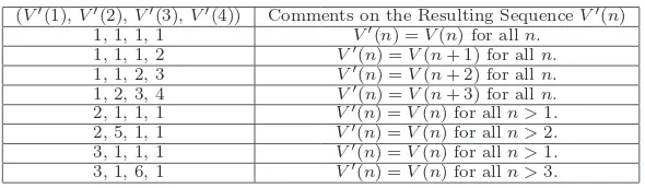
V(1)<5,V(2)<6,V(3) <7 and V(4)<5. In most cases the new initial conditions result in a sequence that becomes undefined (“dies”) relatively quickly. However, there are some interesting exceptions, which we summarize in Tables 10and 11. For clarity in these tables we denote the sequence generated by (3) with new initial conditions byV′
(n). By V(n) we continue to mean (3) with initial conditions all 1s.
Table 10: Recursion (3) with alternative initial conditions that result in a well defined sequence
(V′(1),V′(2),V′(3),V′(4)) Comments on the Resulting SequenceV′(n) 1, 1, 1, 1 V′(n) =V(n) for alln.
1, 1, 1, 2 V′(n) =V(n+ 1) for alln. 1, 1, 2, 3 V′(n) =V(n+ 2) for alln. 1, 2, 3, 4 V′(n) =V(n+ 3) for alln. 2, 1, 1, 1 V′(n) =V(n) for alln >1. 2, 5, 1, 1 V′(n) =V(n) for alln >2. 3, 1, 1, 1 V′(n) =V(n) for alln >1. 3, 1, 6, 1 V′(n) =V(n) for alln >3.
In Table 10 we show the 8 sets of initial conditions, including the original set of all 1s, that result in a well-defined sequence. What is somewhat surprising is that all of these eight sets of initial conditions yield essentially the same sequence!
We outline the proof briefly. First it is readily seen that the induction argument in Section2used to prove that successive terms ofV(n) increase by 0 or 1 carries over for each of these sets of initial conditions (note that the key requirement is that a base case can be established, and this follows since the sequences all match the original V(n) sequence after at most the first few terms). It follows that in each case the resulting sequence does not die. To show that each of the sequences eventually matches the original V(n) sequence with some shift, we prove a somewhat more general result. Let V(n;B) denote the nth term of
the sequence generated by recursion (3) together with initial conditionsB = (b1, b2, b3, b4). Notice that V(n;B) = V(n−V(n−1;B);B) +V(n−V(n−4;B);B). Then the following result holds.
Proposition 26. Let B1 and B2 be two different sets of four initial conditions. Assume
integer N such that V(N +j;B1) = V(j;B2) for 1 ≤ j ≤ 4. Then for all n > 0, we have
V(N +n;B1) =V(n;B2).
That is, if the sequence V(n;B2) has four initial conditions B2 that exactly match a
string of four consecutive values starting at the(N+ 1)th term in the sequenceV(n;B1)then
the sequence V(n;B2) is just the sequence V(n;B1)with the first N terms dropped off.
Proposition26applies directly to a number of the cases in Table10. The initial conditions (1, 1, 1, 2) match a string of four consecutive values of the original V-sequence beginning at the second term of the sequence. In this case these initial conditions lead to the original
V-sequence with one term at the beginning dropped off. The initial conditions (1, 2, 3, 4) match a string of four consecutive values of the originalV-sequence beginning at the fourth term of the sequence. In this case these initial conditions lead to the original V-sequence with three terms at the beginning dropped off.
Proof. We proceed by induction. Assume thatV(N+j;B1) = V(j;B2) forj up tok−1≥4.
Then forj =k we have
V(N+k;B1) = V(N+k−V(N+k−1;B1);B1) +V(N+k−V(N+k−4;B1);B1) (26)
and
V(k;B2) =V(k−V(k−1;B2);B2) +V(k−V(k−4;B2);B2). (27)
By the induction assumption we haveV(N+k−1;B1) =V(k−1;B2) andV(N+k−4;B1) =
V(k−4;B2). Thus we rewrite (26) as
V(N+k;B1) =V(N +k−V(k−1;B2);B1) +V(N +k−V(k−4;B2);B1) (28)
Since V(k;B2) is well defined we know that 1 ≤ k − V(k − 1;B2) ≤ k − 1 and 1 ≤
k−V(k−4;B2)≤k−1. Applying the induction assumption once again to (28) yields
V(N +k;B1) =V(k−V(k−1;B2);B2) +V(k−V(k−4;B2);B2) =V(k;B2). (29)
This completes the induction step and the proof.
Proposition26does not apply directly to all of the cases in Table10. However the proof for these cases follows by using it in two steps. For example, notice that for the set of initial conditions (2, 5, 1, 1) the next three terms of the sequence are 2, 3, 4. We already know that this sequence does not die. Hence we can apply Proposition 26 with B1 = (2, 5, 1, 1) and B2 = (1, 2, 3, 4) to conclude that the two sequences are essentially identical. But since we have already shown that the latter sequence is essentially identical to the original V(n) sequence, we are done. This approach can be used for all the remaining cases (2, 1, 1, 1), (3, 1, 1, 1), and (3, 1, 6, 1).
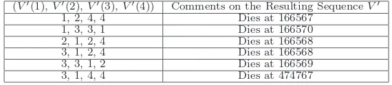
We have already observed that there are only eight sets of initial conditions that together with (3) generate a sequence that does not die. In most cases, if a sequence dies it does so relatively quickly. However, this is not always the case. As we show in Table11, some of the sequences that eventually die do so only after a relatively long life. (Note that in Table 11
Table 11: Examples of recursion (3) with alternative initial conditions that result in sequences that die after a very long life
(V′(1),V′(2),V′(3),V′(4)) Comments on the Resulting SequenceV′ 1, 2, 4, 4 Dies at 166567
1, 3, 3, 1 Dies at 166570 2, 1, 2, 4 Dies at 166568 3, 1, 2, 4 Dies at 166568 3, 3, 1, 2 Dies at 166569 3, 1, 4, 4 Dies at 474767
6
Concluding Remarks
One possible direction in which these results might be extended would be to introduce “shift parameters”a and b as follows:
V(n) = V(n−a−V(n−1)) +V(n−b−V(n−4)) (30)
Such parameters have generated some interesting results in the context of other meta-Fibonacci recursions. We have not explored the values of a and b and sets of initial conditions, if any, for which the sequence V(n) defined by (30) does not die.
Adding additional terms to recursion (3) or (30) offers another possibility. We have confirmed that adding a third term V(n−V(n−7)), together with the initial conditions
V(1) = V(2) = · · ·=V(6) = V(7) = 1 produces a sequence that dies quickly. We have not explored this extension with any other sets of initial conditions, nor what happens if four or more such terms appear on the right-hand side of (3).
Acknowledgements
The authors thank Yuwei Sun for his substantial assistance in the preparation of this manuscript, and Professors Doug Hofstadter and Greg Huber for generously sharing their insights onV(n) and for commenting on earlier versions of this paper.
References
[1] J. Callaghan, J. J. Chew and S. M. Tanny, On the behavior of a family of meta-Fibonacci sequences, SIAM J. Discrete Math. 18 (2005), 794–824.
[2] B. Dalton and S. M. Tanny, Generational structure of meta-Fibonacci sequences,
unpub-lished (2005).
[3] R. L. Graham, D. E. Knuth, and O. Patashnik, Concrete Mathematics, Second Edition, Addision-Wesley, Massachusetts, 1994.
[5] J. Higham and S. M. Tanny, A tamely chaotic meta-Fibonacci sequence, Congressus
Numerantium 99 (1994), 67–94.
[6] J. Higham and S. M. Tanny, More well-behaved meta-Fibonacci sequences, Congressus
Numerantium 98 (1993), 3–17.
[7] D. Hofstadter, Godel, Escher, Bach. An Eternal Golden Braid, Basic Books, New York, 1979.
[8] D. Hofstadter and G. Huber, Private communications and seminar at University of Toronto, March 2000.
[9] T. Kubo and R. Vakil, On Conway’s recursive sequence, Discrete Math. 152 (1996), 225–252.
[10] C. L. Mallows, Conway’s challenge sequence, Amer. Math. Monthly 98 (1991), 5–20.
[11] K. Pinn, Order and chaos in Hofstadter’s Q(n) sequence,Complexity 4 (1999), 41–46.
[12] K. Pinn, A chaotic cousin of Conway’s recursive sequence,Experiment. Math. 9(2000), 55–66.
[13] N. J. A. Sloane, Online Encyclopedia of Integer Sequences,
http://www.research.att.com/∼njas/sequences.
[14] S. M. Tanny, A well-behaved cousin of the Hofstadter sequence, Discrete Math. 105
(1992), 227–239.
2000 Mathematics Subject Classification: Primary 05A15; Secondary 11B37, 11B39.
Keywords: meta-Fibonacci recursion, Hofstadter sequence.
(Concerned with sequences A004001 A005185 A063882 and A087777 .)
Received April 11 2007; revised version received June 26 2007. Published in Journal of
Integer Sequences, June 27 2007.
![Table 6: Values of the frequency sequence at the start and endpoints of the intervals [2k,2k+1−1].](https://thumb-ap.123doks.com/thumbv2/123dok/940750.906563/17.612.238.387.401.496/table-values-frequency-sequence-start-endpoints-intervals-k.webp)