in PROBABILITY
DICHOTOMY IN A SCALING LIMIT UNDER WIENER
MEASURE WITH DENSITY
TADAHISA FUNAKI1
The University of Tokyo, Komaba, Tokyo 153-8914, JAPAN email: [email protected]
Submitted 3 January 2007, accepted in final form 7 May 2007 AMS 2000 Subject classification: 60F10, 82B24, 82B31
Keywords: Large deviation principle, minimizers, pinned Wiener measure, scaling limit, con-centration
Abstract
In general, if the large deviation principle holds for a sequence of probability measures and its rate functional admits a unique minimizer, then the measures asymptotically concentrate in its neighborhood so that the law of large numbers follows. This paper discusses the situation that the rate functional has two distinct minimizers, for a simple model described by the pinned Wiener measures with certain densities involving a scaling. We study their asymptotic behavior and determine to which minimizers they converge based on a more precise investigation than the large deviation’s level.
1
Introduction and results
This paper deals with a sequence of probability measures {µN}N=1,2,... on the space C =
C(I,R), I = [0,1] defined from the pinned Wiener measures involving a proper scaling with densities determined by a class of potentialsW. The large deviation principle (LDP) is easily established for {µN} and the unnormalized rate functional is given by ΣW; see (1.3) below. The aim of the present paper is to prove the law of large numbers (LLN) for {µN} under the situation that ΣW admits two minimizers ¯hand ˆh. We will specify the conditions for the potentialsW, under which the limit points underµN are either ¯hor ˆhasN → ∞.
1.1
Model
Let ν0,0 be the law on the spaceC of the Brownian bridge such that x(0) = x(1) = 0. The
canonical coordinate of x ∈ C is described by x = {x(t);t ∈ I}. For a, b ∈ R, x ∈ C and
N = 1,2, . . ., we set
hN(t) = √1
Nx(t) + ¯h(t), t∈I, (1.1)
1RESEARCH PARTLY SUPPORTED BY THE JSPS, GRANT-IN-AIDS FOR SCIENTIFIC RESEARCH
(A) 18204007 AND FOR EXPLORATORY RESEARCH 17654020
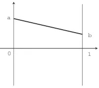
where ¯h= ¯ha,b is the straight line connecting a and b, i.e. ¯h(t) = (1−t)a+tb, t ∈ I; see Figure 1 below. The law onC ofhN withxdistributed underν0
,0 is denoted byνN =νN,a,b. In other words, νN is the law of the Brownian bridge connecting a and b with covariance
EνN[x(t1)x(t2)]−EνN[x(t1)]EνN[x(t2)] = (t1∧t2−t1t2)/N, t1, t2∈I.
LetW =W(r) be a (measurable) function onRsatisfying the condition:
There exists A >0 such that lim
r→∞W(r) = 0,r→−∞lim W(r) =−Aand
−A≤W(r)≤0 for everyr∈R. (W.1)
We consider the distributionµN =µN,a,bonC defined by
µN(dh) = 1
ZN exp
−N
Z
I
W(N h(t))dt
νN(dh), (1.2)
where ZN is the normalizing constant. Under µN,a,b, negative hhas an advantage since the density becomes larger if it takes negative values. This causes a competition, especially when
a, b >0, between the effect of the potentialW pushinghto the negative side and the boundary conditionsa, bkeepinghat the positive side.
The model introduced here can be regarded as a continuous analog of the so-called∇ϕinterface model in one dimension under a macroscopic scaling; see Section 3.
1.2
LDP and LLN
The LDP holds for µN onC as N → ∞under the uniform topology. The speed isN and its unnormalized rate functional is given by
ΣW(h) = 1 2
Z
I ˙
h2(t)dt−A
{t∈I;h(t)≤0}
, (1.3)
for h ∈ H1
a,b(I), i.e., for absolutely continuous h with derivatives ˙h(t) = dh/dt ∈ L2(I) satisfying h(0) = a andh(1) = b, where |{· · · }| stands for the Lebesgue measure. For more precise formulation, see Theorem 6.4 in [2] for a discrete model. Under our continuous setting, the proof is essentially the same or even easier than that. Indeed, whenW = 0, the LDP follows from Schilder’s theorem, while, whenW 6= 0,W(N h(t)) in (1.2) behaves as−A1{h(t)≤0} from the condition (W.1) and can be regarded as a weak perturbation. We omit the details. The LDP immediately implies the concentration property for µN:
lim
N→∞µN dist∞(h N,
HW)≤δ
= 1 (1.4)
for every δ > 0, where HW ={h∗; minimizers of ΣW} and dist∞ denotes the distance inC under the uniform normk · k∞. In particular, if ΣW has a unique minimizerh∗, then the LLN holds under µN:
lim
N→∞µN(kh N
−h∗k∞≤δ) = 1 (1.5)
1.3
Structure of
H
WIt is easy to see that HW = {h¯} when a, b ≤ 0, and HW = {hˇ} when a > 0, b < 0 (or
a <0, b >0), where ˇhis a certain line connectingaandb with a single corner at the level 0; see Section 6.3, Case 2 in [2] for details. The interesting situation arises whena >0, b≥0 (or
a≥0, b >0).
We now assume that a, b > 0. The straight line ¯his always a possible minimizer of ΣW. If
a+b <√2A, there is another possible minimizer ˆhof ΣW. Indeed, let ˆhbe the curve composed of three straight line segments connecting four points (0, a), P1(t1,0), P2(1−t2,0) and (1, b) in this order; see Figure 2. The angles at two cornersP1 andP2 are both equal toθ∈[0, π/2], which is determined by the Young’s relation (free boundary condition): tanθ =√2A. More precisely saying, we havet1=a/√2A, t2=b/√2A witht1+t2<1 (froma+b <√2A), and
ˆ
h(t) =
a−√2A t, t∈I1= [0, t1],
0, t∈I2= [t1,1−t2], b−√2A(1−t), t∈I3= [1−t2,1].
Then, {¯h,ˆh} is the set of all critical points of ΣW (see Section 6.3, Case 1 in [2]), and this implies thatHW ⊂ {¯h,ˆh}.
0 1
a
b
Figure 1: The function ¯h.
0 1
a
b
P1 P2
Figure 2: The function ˆh.
1.4
Results
This paper is concerned with the critical case where both ¯hand ˆhare minimizers of ΣW, i.e. ΣW(¯h) = ΣW(ˆh); note that ΣW(¯h) = (a−b)2/2 and ΣW(ˆh) =√2A(a+b)−A. In fact, in the following, we always assume the conditions (W.1) and
a, b >0 and ΣW(¯h) = ΣW(ˆh), (W.2)
which is actually equivalent to the condition: a, b >0 and√a+√b= (2A)1/4; see Appendix
B of [1].
Theorem 1.1. (Concentration on¯h)In addition to the conditions (W.1)and(W.2), if
W(r) = 0 for allr≥K (W.3)
Theorem 1.2. (Concentration on ˆh)In addition to (W.1)and (W.2), if the following three conditions
∃λ1, α1>0such that W(r)∼ −λ1r−α1 (i.e. the ratio tends to1) asr→ ∞ (W.4)
∃λ2, α2>0such that W(r)≤ −A+λ2|r|−α2 asr→ −∞ (W.5)
0< α1<min{α2/(α2+ 1), α2/2} and Z
I1∪I3
ˆ
h(t)−α1dt >
Z
I ¯
h(t)−α1dt (W.6)
are fulfilled, then (1.5)holds withh∗= ˆh.
The rate functional ΣW of the LDP is determined only from the limit valuesW(±∞), but for Theorems 1.1 and 1.2 we need more delicate information on the asymptotic properties of W
as r → ±∞to control the next order to the LDP. The roles of the above conditions might be explained in a rather intuitive way as follows: The condition (W.3) (with K = 0) means that W is large at least for r≥0 so that the force pushing the Brownian path downward is weak and not enough to push it down to the level of ˆh. On the other hand in Theorem 1.2, since the values of N h(t) in (1.2) are very large fort close to 0 or 1, compared with (W.3), the Brownian path is pushed downward because of the condition (W.4) and, once it reaches near the level 0, the condition (W.5) forces it to stay there. This makes the Brownian path reach the level of ˆh. In the special case where a = b = p
A/8 (t1 = t2 = 1/4), the second condition in (W.6) is fulfilled if 1/2< α1<1, and suchα1, which simultaneously satisfies the first condition in (W.6), exists if α2>1.
Section 2 gives the proofs of Theorems 1.1 and 1.2. Section 3 explains the relation between the (continuous) model discussed in this paper and the so-called∇ϕinterface model (discrete model) in one dimension in a rather informal manner. The analysis is, in general, simpler for continuous models than discrete models. The same kind of problem is discussed for weakly pinned Gaussian random walks, which may involve hard walls, by [1] in which the coexistence of ¯hand ˆhin the limit is established under a certain situation; see also [3]. In our setting, the pinning effect can be generated from potentials having compact supports and taking negative values near r= 0. Our condition (W.1) onW excludes the potentials of pinning type and of hard wall type.
2
Proofs
From (1.4) followed by LDP together with our basic assumption HW ={¯h,ˆh}, for the proofs of Theorems 1.1 and 1.2, it is sufficient to show that the ratio of probabilities
µN(khN−hˆk∞≤δ)
µN(khN−h¯k∞≤δ)
converges either to 0 or to +∞, respectively, asN → ∞for small enoughδ >0. This will be established by (2.2) and (2.3) for Theorem 1.1 and by (2.5)–(2.7) for Theorem 1.2, below.
2.1
Proof of Theorem 1.1
Then, from the condition (W.3) withK= 0, the strong Markov property ofhN(t) underν
∞ ≤δ. However, in the first term, the conditions (W.1) and (W.3) with
K= 0 imply that
whereτ is the hitting time to 0. Therefore the conclusion of the lemma follows from
This lemma, combined with the above computations, shows that for someC >0 (since the LDP holds forνN with speedNand the unnormalized rate functional Σ0(h)), we have that
Thus, the conclusion of Theorem 1.1 follows from (2.2) and (2.3) noting that (1.4) holds with
HW ={¯h,hˆ}.
2.2
Proof of Theorem 1.2
From the definition (1.2) ofµN and by recalling (1.1), we have
The third line follows by means of the Cameron-Martin formula for ν0,0 transforming x+
√
N(¯h−ˆh) into x. However, since ˙¯h(t)≡b−aandR
Ih˙ˆ(t)dt= ˆh(1)−hˆ(0) =b−a, we have 1
2 Z
I
( ˙¯h−h˙ˆ)2(t)dt=−ΣW(¯h) + ΣW(ˆh) +A(1−t1−t2) =A|I2|,
by the condition (W.2). Moreover, sinceh˙ˆ=−√2AonI◦
1, 0 on I2◦ and
√
2AonI◦
3,
Z
I
( ˙¯h−h˙ˆ)(t)dx(t)
= (b−a)(x(1)−x(0)) +√2A(x(t1)−x(0))−√2A(x(1)−x(1−t2)) =√2A(x(t1) +x(1−t2)),
recall thatx(0) =x(1) = 0 underν0,0. Therefore, we can rewrite ˆFN(x) as
ˆ
FN(x) =−N Z
I1∪I3
W √N x(t) +Nhˆ(t)
dt
+√2AN x(t1) +x(1−t2)
−N
Z
I2
W √N x(t)
+A dt
=:FN(1)(x) +FN(2)(x) +FN(3)(x).
To give a lower bound on FN(1), we consider subintervals ˜I1 = [0, t1−p2/A δ] and ˜I3 = [1−t2+p2/A δ,1] ofI1 andI3, respectively. Then, on the eventA1 ={kxk∞≤
√
N δ}, we have fort∈I1˜ ∪I3˜,
√
N x(t) +Nˆh(t)≥ −N δ+Nˆh(t)≥N δ −→ ∞ (asN → ∞),
and also √N x(t) +Nˆh(t) ≤ N(ˆh(t) +δ). Accordingly, by the condition (W.4), for every sufficiently smallǫ >0, the integrand ofFN(1) times−N is bounded from below as
−N W √N x(t) +Nˆh(t)
≥(λ1−ǫ)N1−α1(ˆh(t) +δ)−α1,
which implies, by recalling−W ≥0, that
FN(1)≥(λ1−ǫ)N1−α1
Z
˜
I1∪I˜3
(ˆh(t) +δ)−α1dt=: (λ1−ǫ)C1(δ)N1−α1,
onA1for sufficiently largeN.
To give lower bounds onFN(2) andFN(3), we introduce two more events
A2={x(t1)≥0, x(1−t2)≥0},
A3={x(t)≤ −N−κ for allt∈I2˜ := [t1+N−
1
2−κ,1−t2−N− 1 2−κ]},
where 0< κ <1/2 will be chosen later. Then, obviouslyFN(2) ≥0 onA2. If x∈ A3, noting
that−W(r)−A≥ −Afor allr∈R, we have from (W.5)
FN(3)≥ −2AN12−κ+N
Z
˜
I2
−W √N x(t)
−A dt
for sufficiently largeN. These estimates on FN(1), F
Lemma 2.2. There existsC >0 such that
ν0,0(A2∩ A3)≥CN−
1
2−2κexp{−36N 1 2−κ}.
Proof. Consider an auxiliary event
A4={x(t1+N−
1
2−κ), x(1−t2−N− 1
2−κ)∈[−3N−κ,−2N−κ]}.
Then, by the Markov property, we have
ν0,0(A2∩ A3)≥ν0,0(A2∩ A3∩ A4)
for sufficiently largeN withC1, C2>0. Indeed, the first line is a consequence of
x(t1) =α+B(N−12−κ)−X, X := N
in law whereB(t) is the standard Brownian motion, the second line is seen by the scaling law ofB and 6N−κ≥ −2α, −α≥2N−κ onA
where ¯t=|I2˜| = 1−t1−t2−2N−1
2−κandC3>0. The first inequality is because the straight
line connectingαandβ stays below−2N−κ onA
4. The second line follows from the scaling
law of the Brownian bridge, while the third line is shown by noting thatx(t) =B(t)−tB(1) in law. The last inequality is simple because the distribution of maxt∈I|B(t)| admits a positive and continuous density. Therefore, we obtain
ν0,0(A2∩ A3)≥C4Nκ−
with someC5, C6>0. This completes the proof of the lemma. Since Lemma 2.2 shows
the first condition in (W.6), which implies thatα1(1 + 1
α2)<1 and
1 2−
α1
α2 >0.
On the other hand, we have
Remark 2.1. In the proof of Theorem1.2, the conditions (W.1)and(W.4)are used to show that FN(1) ≥(λ1−ǫ)C1(δ)N1−α1 andF¯
N ≤(λ1+ǫ)C2(δ)N1−α1, while the conditions (W.5) and(W.6)are necessary to prove that the other terms, likeFN(3), ν0,0(A2∩ A3)are negligible.
3
Discussions
Finally, this section makes a remark on the relation between the probability measure µN defined by (1.2) and the so-called∇ϕinterface model in one dimension.
When a symmetric convex potentialV :R→Ris given, to each (microscopic) interface height variable φ={φi}Ni=1−1∈RN−1 satisfying the boundary condition φ0 =aN andφN =bN, an interfacial energyHN(φ) =HNW(φ) called a Hamiltonian is assigned by
HN(φ) = N X
i=1
V(φi−φi−1) +
N−1
X
i=1
W(φi).
Then the statistical ensemble for φis defined by the (finite volume) Gibbs measure
˜
µN(dφ) = 1 ˜
ZN exp
−HN(φ) N−1
Y
i=1
dφi, (3.1)
where ˜ZN is the normalizing constant. We associate a macroscopic height variable{hN(t);t∈
I}with the microscopic oneφby the linear interpolation ofhN(i/N) =N−1φ
i, i= 0,1, . . . , N. Note that, under this scaling, if we especially takeV(η) =η2/2,H
N(φ) is transformed into
˜
HN(h) = 1 2
N X
i=1
N2 h(i/N)−h((i−1)/N)2 +
N−1
X
i=1
W(N h(i/N)),
where we write hN ash. One can thus expect that ˜H
N(h) behaves as
N
1 2 Z
I
( ˙h)2(t)dt+ Z
I
W(N h(t))dt
under the limitN→ ∞. In other words,µN defined by (1.2) may be regarded as the continuous analog of ˜µN introduced in (3.1) under the scaling mentioned above. In fact, this is true in the sense that the errors in the probabilities in the discrete and continuous settings are superexponentially small and behave like e−CN2, C > 0 as N → ∞ (see [7] or the proof of Lemma 6.6 in [2]).
Remark 3.1. The LDP was studied by [4] for the ∇ϕ interface model on a d-dimensional large lattice domain with general convex potential V and the weak self potentialW satisfying the condition (W.1). The variational problem minimizing the corresponding rate functional ΣW naturally leads to the free boundary problem.
References
[1] E. Bolthausen, T. Funaki and T. Otobe. Concentration under scaling limits for weakly pinned Gaussian random walks. preprint, 2007.
[2] T. Funaki. Stochastic Interface Models. Lectures on Probability Theory and Statistics, Ecole d’Et´e de Probabilit´es de Saint-Flour XXXIII - 2003 (ed. J. Picard), 103–274, Lect. Notes Math.,1869(2005), Springer. MR2228384 MR2228384
[3] T. Funaki. A scaling limit for weakly pinned Gaussian random walks. submitted to the Proceedings of RIMS Workshop on Stochastic Analysis and Applications, German-Japanese Symposium, RIMS Kokyuroku Bessatsu.
[4] T. Funaki and H. Sakagawa. Large deviations for∇ϕ interface model and derivation of free boundary problems.Proceedings of Shonan/Kyoto meetings “Stochastic Analysis on Large Scale Interacting Systems”(2002, eds. Funaki and Osada), Adv. Stud. Pure Math., 39, Math. Soc. Japan, 2004, 173–211. MR2073334 MR2073334
[5] I. Karatzas and S.E. Shreve. Brownian motion and stochastic calculus (2nd edition), Springer, 1991. MR1121940 MR1121940
[6] L. Tak´acs. The distribution of the sojourn time for the Brownian excursion.Methodol. Comput. Appl. Probab.,1(1999), 7–28. MR1714672 MR1714672