Directory UMM :Journals:Journal of Operations Management:Vol18.Issue3.Apr2000:

www.elsevier.comrlocaterdsw

Inventory policy for dense retail outlets

Michael Ketzenberg

a

, Richard Metters

b,)

_{, Vicente Vargas}

c

a

Kenan-Flagler Business School, UniÕersity of North Carolina-Chapel Hill, Chapel Hill, NC, USA

b

Cox School of Business, Southern Methodist UniÕersity, Dallas, TX 75275-0333, USA

c

Goizueta Business School, Emory UniÕersity, Atlanta, GA, USA

Received 1 March 1999; accepted 1 September 1999

Abstract

A potential retail operations strategy is to have a ‘‘dense’’ store. That is, a store that combines high product variety with a small footprint. Retail management desires smaller stores to provide the strategic benefits of convenience and speed to customers, but desires larger stores to provide high product variety. Noting the benefits of smaller, more numerous stores, several retailers well known for their extremely large store size recently have begun experimenting with a small store format. Traditional retail inventory management policies, however, have difficulty combining high variety and small store size. Here, the potential advantages of the dense store type are explored. To facilitate this exploration, inventory policies are developed to help manage small stores by increasing their product density. Results based on grocery industry data indicate that the heuristics compare favorably to optimality and permit the dense store concept to potentially achieve substantial gains compared to current practice.q_{2000 Elsevier Science B.V. All rights reserved.}

Keywords: Service operations; Inventory control

1. Introduction

1.1. Anecdotal eÕidence for the ‘‘dense’’ store

strat-egy

In recent years, a number of retail firms have made plans to adopt a ‘‘denser’’ store strategy. We use the term ‘‘density’’ to refer to the number of products or categories that a store provides per unit

)_{Corresponding author. Tel.:}

q1-214-365-0230; faxq 1-214-768-4099.

Ž .

E-mail address: rmetters@mail.cox.smu.edu R. Metters .

of selling space. This desire has taken two different forms. For some, there has been an increase in the number of product categories or individual

stock-Ž .

keeping units SKUs within the same sized store. For others, there has been a desire to reduce store size.

The theory behind increasing category and prod-uct variety is that high variety stores are more attrac-tive to customers as they offer a better opportunity

Ž

for one-stop shopping Messinger and Narasimhan

.

1995, 1997 . The grocery industry provides a fitting example and will be the main subject of this study. The number of SKUs in the average grocery store

Ž

increased 96% from 1980 to 1993 Sansolo and

.

Garry 1994 .

0272-6963r00r$ - see front matterq_{2000 Elsevier Science B.V. All rights reserved.} Ž .

Largely, the grocery industry has accommodated increases in SKUs by increasing store size, as aver-age store size has increased nearly 50% from 1985 to

Ž .

1994 Sansolo and Garry 1994 . However, large stores have several disadvantages well known to retailers: a strategy of a few large stores versus several smaller stores leaves customers with more travel time required to get to a store, usually means more difficulty in parking an automobile close to a store, and requires more search time for customers within a store.

In response to the inherent advantages of keeping stores small, in addition to providing high variety, one of the market leaders in the grocery industry has publicly made ‘‘densing up’’ stores a strategic

prior-Ž .

ity Safeway annual report 1992, p. 9 . Leaders throughout the industry have pursued a strategy of ‘‘combination’’ stores by adding more shelving and product categories to existing stores to incorporate

Ž

more inventory Kroger annual report 1997, Safeway

.

annual report 1997 . Many supermarkets have be-come near shopping malls in their own right, adding pharmacies, florists, dine-in restaurants, etc. In one area of expansion, the number of retail banks in US grocery stores has increased from 210 in 1985 to

Ž .

4400 in 1996 Williams, 1997 .

Examples also abound in other retail industries. Tricon, owner of Pizza Hut, Taco Bell and Kentucky Fried Chicken, has now opened ‘‘multi-concept’’ stores that combine two or even all three of the aforementioned concepts in one physical building

ŽGibson, 1999 . Dollar General, a general merchan-.

dise retailer, recently increased their per store SKUs

Ž .

by 20% Berner, 1998 . Southland has revitalized the 7-11 brand and plans to open a new store a day for

Ž .

the next two or three years Lee, 1998b . A center-piece of their revitalization has been their new Retail Information System which has allowed them to be-come more dense, increasing SKUs per selling area

Ž

an average of 30% Bennett, 1994, Southland

An-.

nual Report 1997 .

Prominent examples of firms that are successful with this format include two general merchandise retailers, Dollar General and Family Dollar. Both chains compete for the same target market as Wal-Mart, both are competitive with Wal-Mart on price, and both have over 3000 stores in the US, yet the average store size is 6000 ft2 _{vs. Wal-Mart’s}

aver-2 _{Ž .}

age 92,000 ft . Berner 1998, Friedman 1998 . One strategy of Dollar General is to locate stores next to existing Wal-Marts to highlight their convenience. Wal-Mart has acknowledged these competitors and has begun experimenting with a ‘‘Small-Mart’’

strat-Ž .

egy of far smaller stores Lee, 1998a . Likewise, Home Depot currently has an average store size of 112,000 ft2, but in 1999, is experimenting with a

Ž .

small-store strategy Hagerty, 1999 and Sears is

Ž .

opening ‘‘compact’’ stores AP, 1998 . A key ques-tion facing these practiques-tioners is how to combine provide enough variety with the small store conve-nience to attract customers.

In the grocery industry, the small-store, but non-dense strategy is generally known as a ‘‘limited assortment’’ strategy. Limited assortment stores gen-erally are 20–40% of the size of the average super-market and stock only a few SKUs in each category. Price competitor chains of over 500 such stores

Ž .

include Aldi, Dia and Save-a-lot e.g., Lewis, 1997 .

Ž .

Other chains, such as Trader Joe’s Los Angeles and

Ž .

Harry’s In A Hurry Atlanta , are upscale competi-tors. These competitors seek to take advantage of their small size, but have the disadvantage of fewer SKUs.

The purpose of this work is to provide the means to manage a dense store. Current retail inventory practices are not adequate to the task. Consequently, we have devised an inventory replenishment policy for the retail sector that supports a dense store format. We place our research in the context of the grocery industry. Inventory practices are known by the industry to be largely inefficient. Consider dry-groceries. In 1993, the average dry-grocery product was sold to customers 104 days after release by the supplier, with 26 of those days sitting in a retail

Ž .

grocery store Kurt Salmon Associates 1993, p. 26 . This concern over inventory and replenishment prac-tices has been expressed in an industry-wide move-ment known as ‘‘Efficient Consumer Response’’

ŽECR . This initiative began in the early 1990s and is. Ž

endorsed by nearly all the major retailers Kurt

.

Salmon Associates 1993 . The tenets of ECR are similar to JIT and time-based competition: the spe-cific goal is ‘‘reducing total system costs, inventories and physical assets while improving the customer’s

Ž .

ŽESA which addresses the optimum use of store and.

shelf space to provide a complete, easy to shop, assortment of products the consumer wants. The idea behind ESA is to enable more space for broader

Ž

assortments per category or for new categories Kurt

.

Salmon Associates, 1993, pp. 42–43 . Our research supports this and provides a new tool to achieve this result.

1.2. The practical impact of replenishment modeling

There are generally three hierarchical levels of retail inventory policy:

Ø assortment — deciding which products should be stocked,

Ø allocation — how much shelf space to give each product in the assortment, and

Ø replenishment — when and how much to reorder.

Historically, researchers addressing the retail in-ventory problem have developed models that focus on determining assortment and allocation, rather than on determining inventory stocking and replenishment

Ž

policies for example, Anderson, 1979; Corstjens and Doyle, 1983; Borin and Farris 1995; Borin et al.,

.

1994 .

The focus here is on finding a simple model for inventory replenishment that enables retail managers to make greater use of their scarce resource: retail space. Methodologically, we construct replenishment heuristics to facilitate category management that are easy to implement. These heuristics are then com-pared to both optimal policies and current practice. We do so utilizing data from a leading national grocer that is a founder of ECR.

For the data studied, the heuristic reduces inven-tory levels 24–50% from current practice while maintaining profitability. This inventory reduction has ramifications for the assortmentrallocation deci-sions, as it lessens the need for shelf space assigned to the current assortment. Given a static store size, this enables higher variety through either the addi-tion of more products in a category or the inclusion of more general categories of goods. Alternatively, the reduction in space needs can lead to smaller stores or more aisles per store.

This paper is organized as follows. Section 2 defines the problem and reviews the relevant litera-ture. This is followed by a description of inventory practice at the grocer in question and heuristic devel-opment. Heuristics are tested against optimal solu-tions by dynamic programming in a restricted envi-ronment. Then the heuristics are tested under more realistic business conditions by simulation.

2. Problem definition and literature review

The general setting is a retail facility under peri-odic inventory review that stocks multiple, substi-tutable products to satisfy stochastic demand. In each time period, the stocking level of any product is restricted because of shelf space allocation decisions made previously. Given a set assortment and alloca-tion scheme, the problem then is to determine the amounts to be ordered in each period so as to maximize profit, where profit is calculated as rev-enue less the purchasing cost, inventory storage cost, and penalties for substitution and lost sales.

Ordering costs are not included as there is little marginal ordering cost for a given product. As de-scribed in detail later, product orders take seconds of employee time to note and transmit electronically, only minutes to kit at a distribution facility, and are loaded onto a common truck filled with hundreds of other orders so there is no marginal transportation cost. As technology improves, ordering costs are likely to decrease from this small amount. One can imagine inventory position being decremented auto-matically from scanner data captured at the point of sale and the ordering process being computerized to the degree where in-store employees are omitted entirely from the ordering process.

Given a stockout situation in one product, we presume that a known proportion of consumers who originally intended to buy that product will desire to purchase another product as a substitute. As a practi-cal matter, substitutability as a percentage of retail out-of-stock situations has been variously estimated

Ž

from empirical data at virtually 100% Motes and

. Ž .

Castleberry, 1985 , 84% Walter and Grabner, 1975 ,

Ž . Ž

82% Walter and La Londe, 1975 , 73%

Em-. Ž .

Ž .

40% Nielsen Marketing Research, 1992 depending on the specific retail environment. Product substi-tutability is important for the replenishment decision as it can act in a similar fashion to the pooling of inventory at a central warehouse; substitutability

re-Ž

duces the need for inventory McGillvray and Silver,

.

1978; Moinzadeh and Ingene, 1993 .

In Appendix A, we develop a dynamic program-ming formulation of the replenishment problem. The purpose of developing the formulation is to both link this problem to prior literature and facilitate heuristic comparison to optimal policies for simple cases in-volving two products. Beyond a few products, opti-mal solutions for substitutable products are impracti-cal for dynamic programming as the state space

Ž .

expands exponentially Smith and Agrawal, 2000 . The following notation is useful in mathemati-cally describing the replenishment problem and con-structing heuristics. the target inventory position on hand after ordering

Ž

but before demand a target that will often not be

. Ž .

reached due to case–pack sizes and is i ,i , . . . i_{1 2 p}

is the vector of inventory positions at the beginning of the order cycle. Due to the nature of retail de-mand, we assume that excess demand results in either lost sales or sales of another product, so

ijG0.

We define the following parameters for each product j. Let sjksproportion of unfilled demand

Ž .

that may be filled by substituting product k si j'0 ,

SsÝp

s the overall substitutability factor, 0F

j ks1 jk,

SF1, Õsrevenue per unit, h sholding cost per

j j j

unit per period, pj_spenalty cost per unit of stock-out, c_jspurchase cost per unit, R_jsmaximum units of product that space allocation allows on the shelf,

Ž .

and f x sthe joint probability mass function of

Ž .

demand, where xs x , x , . . . , x_{1 2 p} denotes a partic-ular realization of demand.

Finally, Kjscase–pack size. Products cannot be ordered as individual units. They must be ordered in manufacturer prepared ‘‘case–packs’’ of several units each.

Simpler versions of this problem can be solved readily. If case–pack considerations are eliminated and substitutability is zero, traditional marginal

anal-Ž .

ysis is known to be optimal Karr and Geisler 1956 . If the case–pack size is one and there is no substi-tutability, we have a multi-period news vendor prob-lem where the form of the solution is a single critical order-up-to number for each product.

Given a case–pack size greater than one, the optimal solution is known to be a single critical reorder point with a target order-up-to point for each product. Note that the Y inventory target can only_j be attained when Y_jyi is a precise multiple of the_j

case–pack size. Setting Y as a maximum target is_j consistent with prior literature on batch ordering

ŽVeinott, 1965 . Given the complexity of the prob-.

lem, the form of the solution is not known and the behavior and calculation of optimal solutions and approximating heuristics have not been explored. Consequently, an additional contribution that this manuscript makes is in investigating the behavior of such systems and developing heuristics. These heuristics are relatively simple, lead to good solu-tions and provide substantial improvement over cur-rent practice.

3. Current practice

3.1. An empirical example: existing logistics and inÕentory practices

This study explores retail inventory management by means of a specific example in the grocery industry. We utilize data from what is known in the trade as the ‘‘oil and shortening’’ category of a store in a leading national grocery chain.

Transportation and logistics have benefited from JIT-based enhancements. Stores can receive product shipments in the oil and shortening category five times weekly as opposed to once a week a decade ago. Delivery lead time is two days. Orders are processed and transmitted electronically between stores and the regional warehouses that resupply them.

SKU to determine whether a case–pack of the item would fit in the space left vacant by item sales. If so, an order is placed.

As suggested above, inventory policy calls for each product to fill the entire depth of the shelf. The reason given for this policy was to reduce the cost of inventory at the warehouse. However, it is clear that while this may reduce the inventory cost at one location, overall inventory investment is not reduced. This inventory policy does simplify ordering, how-ever, as a visual estimation of the amount of empty shelf space is the only decision required.

The company in question does not have a ‘‘state of the art’’ replenishment system. At the current time scanner based inventory control is still considered too inaccurate to pursue. For a description of a more technologically advanced operating system, we refer

Ž .

the reader to McKenney et al. 1994 and Garry

Ž1996 . It is anticipated that this system will become.

more automated in the future.

3.2. Analyzing an existing shelf set

The oil and shortening category occupies 86 lin-ear feet of shelf space on five separate shelves. The information requirements for analyzing shelf set per-formance were difficult to obtain. Data were ob-tained from multiple, disparate, and isolated com-puter systems. Some data, such as product cost, were only available on manually filed historical order records. Product physical dimensions had to be mea-sured by hand. This is typical of the industry.

A total of 93 distinct SKUs were on display. For a number of products insufficient information was available from store records. As a result, 77 of the 93 possible SKUs, comprising 239 product facings and

Ž

70 linear shelf feet, are used in this study. A product ‘‘facing’’ refers to the front row on a shelf, the only

.

row of product ‘‘facing’’ the customer . Summary statistics on these products are in Table 1.

There is substantial variance throughout the cate-gory on each of the measures noted in Table 1. The average case–pack size is 9, but 15 items can be resupplied individually while 34 items have case– pack sizes of 12 to 24.

The average gross margin reported here is 43%, which is consistent throughout the industry in dry goods. In the mind of the public the profit margin for

Ž .

grocery stores is about 1% e.g., Coleman, 1997 . However, this ‘‘profit’’ margin is income netted against all expenses — including the proverbial pres-ident’s jet.

Demand differs strongly between products. Six-teen products sell two or less units per week while 43 products average daily unit movement. This is somewhat more homogeneous than the industry av-erage, where 56% of dry grocery items average less than one unit sales per week and 22% of items

Ž

average at least one unit per day Kurt Salmon

.

Associates, 1993, p. 27 .

Considering the frequent delivery schedule, inven-tory levels appear high. This excess is emblematic of retailing in general. An industry average of 26 days

Ž

of inventory of dry grocery items is on display Kurt

.

Salmon Associates, 1993, p. 26 . Inventories of cos-metics at department stores often turn over twice

Ž .

yearly Seshadri, 1996 and retail clothing stores set inventory levels at nearly 100% service levels by

Ž

stocking several weeks of demand Agrawal and

.

Smith, 1996 .

Due to relative profitability levels and the influ-ence of case–pack sizes, these inventory levels are not as unreasonable as they appear.

Throughout the retail sector, SKUs that have low sales volume are included in the assortment. Agrawal

Ž .

and Smith 1996 found that two-thirds of the SKUs in retail clothing sell less than one per week. But low-demand SKUs are still profitable. Given the profitability data on Table 1 and assuming holding costs of 25% annually, the profits from a one-unit sale are nearly equivalent to the costs of holding a unit for two years. For these items, case–pack size creates large inventory values relative to demand. Given a case–pack size of 12 and an average de-mand of one per month inventory turns will not be high.

Safety stock can be large for high demand items as well. Assume inventory decisions are based on a newsvendor inventory model. The cost of under-stocking, C , could be construed as the averageu

profit margin above plus, say, 50% of the margin as a penalty cost of lost sales. Assume C , the cost of_o overstocking, to be represented by an annual holding cost of 25% of the item cost. The service level that

Ž .

Table 1

Category summary

Case–pack Price Cost Percent Weekly Maximum Days supply of

a b

ŽUS$. ŽUS$. margin %Ž . sales inventory inventory

Mean 9 2.92 2.02 43 10 22 28

Standard deviation 6 2.34 1.27 32 9 14 31

20th percentile 1 1.79 1.17 21 2 8 9

40th percentile 8 2.10 1.60 31 6 15 15

60th percentile 12 2.59 1.81 43 9 20 22

80th percentile 12 3.09 2.24 54 15 30 35

a

Inventory level when all facings allocated to an SKU are full of product.

b

Days supply of product at the maximum inventory level. This measure does not equal the mean maximum inventory divided by mean weekly sales. Mean days supply is the numerical average of the days supply of each product individually.

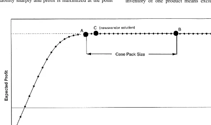
Traditionally there has been little incentive to keep inventories low due to the asymmetric penalties between erring on the low versus high side. Fig. 1 depicts profitability levels of various reorder points assuming the costs on Table 1. Extremely low stock-ing levels cause substantial stockouts and provide a negative return. Adding inventory increases prof-itability sharply and profit is maximized at the point

shown. Because of the high ratio between profits and holding costs adding large amounts of inventory in excess of the profit maximizing point produces only negligible profitability deterioration.

This traditional view of inventory management, however, neglects the issue of space utilization. Given finite space for a category, including more inventory of one product means excluding another

product entirely, thereby reducing the assortment and making the store less attractive to customers. Or, if all items in a category are allowed to stock to nearly 100% customer service levels, fewer categories can be included in a store.

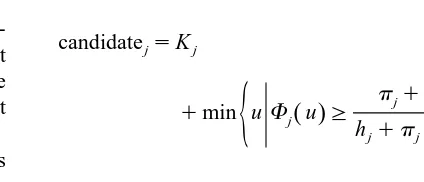
4. Heuristic development

The central ordering question that must be an-swered is the number of case–packs, N , of productj

to order in each time period. We compare two simple heuristics to both optimal solutions and the current practice utilized by the business studied.

We adapt the literature of base-stock policies

Žgenerally, zero ordering cost policies to the case–.

pack environment and derive the ‘‘base-stock’’

Ž .

heuristic BAS . From the literature on case–packs,

Ž .

we take the essential insights from Veinott 1965 , who worked on the single product, back-order prob-lem, and generate the ‘‘Modified Veinott’’ heuristic

ŽMOD to the lost sales. rsubstitution case with mul-tiple items and lead times. In keeping with the notation of the literature on batch ordering, for each heuristic we define a target inventory level Y . Thej

number of cases ordered for a given inventory

posi-Ž ?Ž . Ž .@. ? @

tion is Njsmax 0, Y ijy j r Kj where x indi-cates truncation to an integer value.

Ž .

As a formal heuristic, current practice CP seeks to replicate the managerial emphasis on filling all the available space given by the allocation scheme with product.

( ) 4.1. Current practice heuristic CP

For each product js1, . . . , p, the target inventory level is the maximum stock level,

YjsR .j

Ž .

2

Or, equivalently, R_jyK_j functions as a reorder point. This heuristic has the advantage of operational simplicity — a visual check to see if there is room on the shelf for another case–pack is all that is required.

Some additional notation is useful for the

subse-Ž . ` `

bability mass function for product j, and Fj x

x _{Ž .}

Ýus0fj u , the cumulative marginal demand

distri-bution for product j.

( ) 4.2. Base stock heuristic BAS

For each product j determine the target inventory_, level as follows:

The BAS heuristic calculates a traditional base

Ž .

stock inventory position plus a case–pack 3 so that inventory after ordering is above the traditional base stock reorder point. The target inventory value is

Ž .

subject to a maximum of the shelf capacity 4 . The reason for including the BAS heuristic in this study is due to its benchmark status among researchers, its simplicity in calculation and that it takes into consid-eration the relative profitability of items.

( ) 4.3. Modified Veinott heuristic MOD

The MOD heuristic attempts to consider both case–pack size and substitutability in addition to differential product margins. At the core of the MOD heuristic is the form of the optimal policy for

order-Ž .

ing by case–packs Veinott, 1965 : if expected

prof-Ž .

itability, E Profit , is a unimodal function of inven-tory where the slope changes sign once from positive to negative as inventory positions move from zero to infinity, then the optimal case–pack ordering policy is to order up to, but not over, a point B where

Ž < . Ž < .

E profit y_sB _sE profit y_sB_ycase–pack

ŽFig. 1 . Point B less the case–pack size leaves point.

A as the reorder point. We adapt this fundamental

insight to the partial lost salesrsubstitutability case with positive lead times.

The second approximates the profitability of a given stocking level using the expected sales.

u

x sales– j

Ž .

u s

Ý

ifj

Ž .

i qu 1

Ž

yFj

Ž .

u

.

,

is1

x profit_{– j}

Ž .

u s

Ž

Õ_jyc_j

.

x sales_{– j}

Ž .

u

gross margin

yh uj

Ž

yx sales– j

Ž .

u

.

holding cost

ypj

Ž

mj_yx sales– j

Ž .

u

.

penalty cost

yS

Ž

Õyc

.

x sales_–

Ž .

u ,

j j j j

substitutability

where

`

mj_s

Ý

ifj

Ž .

i ,

is0

is the expected value of demand.

In the formulation of the x profit function, we_– assume that a penalty cost applies when a customer is forced to substitute an item. Given product substi-tutability, however, a sale of one item can be viewed as a decline in sales of another item. Because a consumer usually substitutes within a restricted set, say a premium product for another premium product, the substitutability term in x_profit assumes the same revenue and cost functions of the product at hand. The reverse situation, the additional demand seen due to stockouts of other items, is not consid-ered. This serves to reduce the safety stock held and models the pooling effect of product substitutability discussed earlier, while keeping the model simple to use and understand.

For each product j determine the target inventory level as follows:

differences0, TargetsK ,_j

Reorders1,

While difference G0 and Target -R do begin,j

TargettsReorderqK ,j

Ž .

Target profit_– sx profit_– j Target ,

Ž .

Reorder profit_– sx profit_– j Reorder ,

differencesTarget profit_– yReorder profit,_– if difference-0 then TargetsTargety1, else ReordersReorderq1,

end while,

YjsTarget.

The MOD heuristic is a single pass algorithm for determining case–pack orders. For each product, the default order-up-to target is the minimum possible value that forces the product to be included in the assortment, the case–pack size Kj. The profits asso-ciated with the order-up-to target and reorder point are compared in the value ‘‘difference.’’ As long as the difference is positive the reorder point and target inventory levels increase. They are increased until either the difference becomes negative or the target inventory level reaches shelf capacity.

It should be noted that there are practical limita-tions to the heuristics described above – they cannot reasonably be applied to every product in a store. ‘‘Loss leaders’’ represent a common marketing tech-nique where products are sold below cost. ‘‘Slotting fees’’ are often given to grocers for a minimum shelf requirement. This will not usually present a barrier, since slotting fees are typically given just for being

Ž .

present in a store i.e., receiving a single facing .

5. Experimental design and results: two-product case

5.1. Experimental design

The heuristics are compared to optimality by dy-namic programming in a two-product scenario. Later, in Section 6, we compare heuristics by simulation for the full 77-product category. Dynamic programming is not a practical solution method in this case due to the well-known ‘‘curse of dimensionality.’’ The only reason for using dynamic programming is to give a sense of how distant from optimality each heuristic may be in a limited setting. System parameters for both analyses, such as the product revenues, costs, physical capacities, case–pack sizes, etc., are from actual store data. Actual sales data is used here as the

Ž

‘‘natural’’ demand as opposed to demand stemming

.

Ž .

converted to a demand function e.g., Hill, 1992 . In this case, as also occurred with Agrawal and Smith

Ž_{1996 , the actual inventory levels are so large for all}.

but a few products that this step is not necessary. For the two-product problem, an optimal solution is found and costs are calculated utilizing the dy-namic program in Appendix A. As dydy-namic pro-gramming is used to find exact expected values, statistical analysis is not required for this portion of the experimental design.

Parameters are varied from a base case to explore the effects of parameter changes. The base case assumes two identical products, which have retail prices of US$2.92, cost US$2.02, sell an average of 10 unitsrweek, and have a case–pack size of 9,

Ž

corresponding to the averages on Table 1. For the CP heuristic, the industry average stocking policies

.

cited earlier are used. The substitutability percent-age is assumed to be 70%, holding costs 25% annu-ally of product cost, the lost sales penalty cost is assumed to be 50% of product margin and the penalty for substitution is 10% of the lost sales penalty. A cycle of length 3 days is modeled, roughly corresponding to the case where 3 days of demand can occur before a replenishment is received. In accordance with both analysis of the data and similar work, Poisson demand distributions are assumed for

Ž

the base case e.g., Karr and Geisler, 1956; Hill,

.

1992 .

Ten scenario variations are explored to this base case. The lost sales penalty cost is set to 10% and 200% of product margin. Corresponding to research cited earlier, substitution takes on values of 40% and 100%, and a substitution rate of 0% is also used for comparison. Due to the presence of negative bino-mial distributions noted in retail practice by Agrawal

Ž .

and Smith 1996 , the negative binomial demand distribution is explored. Three values of the vari-ance-to-mean ratio of 1.1, 1.5 and 2, were used for the negative binomial distribution.

5.2. Results

The detailed results from the base case

experi-Ž .

mental cell Table 2 mirror those of all other cells. Gross profits are nearly identical for all policies because each heuristic has a fill rate beyond 99%. The reasons for extreme fill rates for all policies

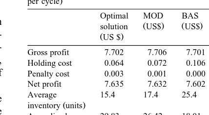
Table 2

Results from the base case experimental cell: substitutability 70%,

Ž

lost sales cost 50% of margin, case–pack sizes9 average costs

.

per cycle

Optimal MOD BAS CP

Ž . Ž . Ž .

solution US$ US$ US$

ŽUS $.

Gross profit 7.702 7.706 7.701 7.704

Holding cost 0.064 0.072 0.106 0.180

Penalty cost 0.003 0.001 0.000 0.000

Net profit 7.635 7.632 7.602 7.524

Average 15.4 17.4 25.4 63.4

Ž .

inventory units

Annualized 29.83 26.42 18.01 7.14

ROII

have been identified earlier: large differences in holding versus lost sales costs and the effect of case–pack sizes. Net profits differ between the heuristics, but the differences are small, amounting to only 1% in the base case.

The results of interest are the average inventory investment and the return on inventory investment

Ž_{ROII , a common industry barometer of effective-}.

Ž .

ness e.g., Thayer, 1991 , and a more useful barome-ter when implementing a dense store strategy. Both of these results follow a clear pattern: in every experimental cell, MOD is the superior heuristic

ŽTable 3 . The reason we focus on ROII rather than.

net income is because of the relative scarcity of retail space. The business implications of policies which achieve higher ROII values are discussed in detail in Section 6, but include the ability to include more products in an assortment, more product categories in a store or allow a reduction in store size.

Perhaps the most striking aspect of Table 3 is the lack of numerical change of ROII results for the BAS and CP heuristics as parameters change. De-creases in substitutability and inDe-creases in penalty costs and demand variance have the effect of increas-ing the probability of product shortages. However, due to reasons discussed earlier concerning industry cost structure, inventory levels are so high for these heuristics that the increased lost sales due to these factors is insufficient to change the ROII for these heuristics to the level of one-hundredth of a point.

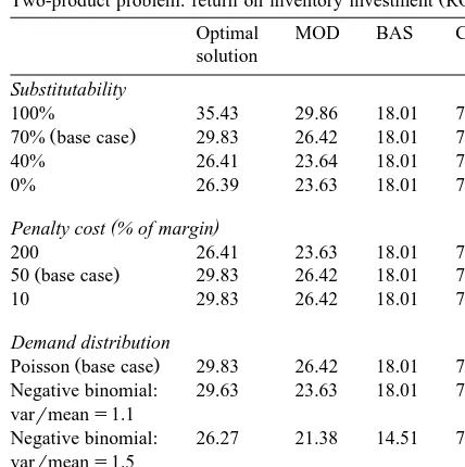
Table 3

Ž .

Two-product problem: return on inventory investment ROII

Optimal MOD BAS CP

solution

Substitutability

100% 35.43 29.86 18.01 7.14

Ž .

70% base case 29.83 26.42 18.01 7.14

40% 26.41 23.64 18.01 7.14

0% 26.39 23.63 18.01 7.14

( )

Penalty cost % of margin

200 26.41 23.63 18.01 7.14

Ž .

50 base case 29.83 26.42 18.01 7.14

10 29.83 26.42 18.01 7.14

Demand distribution

Ž .

Poisson base case 29.83 26.42 18.01 7.14 Negative binomial: 29.63 23.63 18.01 7.14 varrmeans1.1

Negative binomial: 26.27 21.38 14.51 7.14 varrmeans1.5

Negative binomial: 22.33 17.98 12.84 7.14 varrmeans2

parameter values. This is due to the large stockout to penalty cost ratio. Changing substitution rates from 0% to 40% may change the optimal service level from, say, 99.9% to 99.5%, which is insufficient to cause an integral change in the optimal inventory reorder point.

6. Experimental design and results — 77-product simulation

6.1. Experimental design

Here, we simulate the heuristics in the more realistic environment of the 77 products described

earlier. Varied quantities include the penalty cost for lost sales, p_s10%, 50% and 200% of net margin. We assume that the quantities Sj'a constant factor among all products that represents the general substi-tution percentage and employ values Ss40%, 70% and 100%. The individual product substitutability factors, s , are uniformly distributed based on prod-_{i j} uct type: for example, a premium olive oil would only be substituted for other premium olive oils, and all other premium olive oils are considered equally likely to benefit from a stockout. Due to the absence of a strong demand distribution effect in the dynamic program, only the Poisson distribution is used.

Detailed logistics practices are modeled. Deliver-ies occur every day except Saturday and Sunday. The demand pattern varies by day of the week, with Monday through Friday accounting for 13% of weekly demand and Saturday and Sunday for 17% and 18% of weekly demand, respectively, corre-sponding to store sales. There is a lead time of 2 days for ordered product.

Ten replications of 6 years is run for each heuris-tic and experimental cell. Statisheuris-tics are collected after the first simulated year to avoid initialization bias. Total CPU time for all experimental cells is approxi-mately 24 h.

6.2. Results and implications for dense stores

The mean results of a typical experimental cell

ŽTable 4 mirror those seen earlier —- gross and net.

profits are similar but ROII differs considerably be-tween heuristics. Standard errors are small for all entities reported due to the extreme length of time simulated.

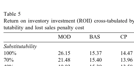
Evaluating the effect on ROII as parameters change, again MOD responds to changes in the substitutability level and is more effective as

substi-Table 4

Ž .

Results from a typical experimental cell: substitutability 100%, lost sales cost 50% of margin annual basis

MOD BAS CP

Ž . Ž . Ž . Ž .

Gross profit mean standard error 28,985 23 28,794 30 28,921 26

Ž . Ž . Ž . Ž .

Holding cost mean standard error 241 0.1 449 0.1 488 0.2

Ž . Ž . Ž . Ž .

Penalty cost mean standard error 28 0.3 40 0.9 83 0.6

Ž . Ž . Ž . Ž .

Net profit mean standard error 28,716 22 28,305 30 28,350 26

Ž . Ž . Ž . Ž .

Average inventory mean standard error 964 0.4 1796 0.6 1951 0.7

Ž . Ž . Ž . Ž .

Ž .

tutability increases Table 5 . Further

experimenta-Ž .

tion not shown indicates that the sensitivity of MOD to parameter values outside the range of the experimental design is not large.

Adoption of the MOD heuristic as a replenish-ment tool assists in achieving the goals of a dense store: either more categories can be offered in the same space, or the same number of categories can be offered in a smaller space. Thus far, we have as-sumed that the allocation of facings to SKUs is given. That is, each heuristic accords the oil and shortening category 239 facings and 70 linear shelf feet. Given the lower inventory levels, however, the MOD heuristic could reduce the number of facings

Ž .

from 239 to 179 Table 6 . This reduction in facings would reduce the number of linear feet required for the 77 products analyzed from 70 to 53 ft.

Given this space reduction and assuming other products have similar characteristics, 103 products could fit in the same space where the 77 original products now reside. Assuming equivalent net profits to the shelf set analyzed, which is optimistic, this could increase annual profitability of those 70 linear ft 38% by adding more SKUs to the category or by adding more categories to the store.

It could be argued that cutting the shelf space of the category may depress category sales. There is ample evidence that shrinking the space of one prod-uct leads to sales shifting to other prodprod-ucts in the category. However, we are not aware of any research that indicates that shrinking the shelf space of all products in all categories simultaneously results in

Ž

category-wide or store-wide revenue reductions a

Table 5

Ž .

Return on inventory investment ROII cross-tabulated by substi-tutability and lost sales penalty cost

MOD BAS CP

Substitutability

100% 26.15 15.37 14.47

70% 21.48 15.40 13.96

40% 19.93 15.39 13.58

Penalty cost

200% of margin 20.79 14.96 13.77

100% of margin 22.45 15.41 14.05

50% of margin 24.32 15.79 14.20

Table 6

Ž

Allocation ramifications of replenishment heuristics

substitutabi-.

lity 100%, lost sales cost 50% of margin

MOD CP

Facings 179 239

Linear shelf feet 53 70

Number of products in 239 facings 103 77 Required shelf depth for 239 facings 16 in. 20 in. Potential profit from 70 linear US$39,130 US$28,350 shelf feet

review of related research is in Mahajan and Van

.

Ryzin, 1999 .

Given the assumption that category-wide sales declines may occur, the MOD heuristic can still assist in increasing variety. Using this heuristic, the same number of facings could be achieved by chang-ing shelf depth from the current 20 to 16 in. Given the extra space, and assuming six feet between aisles, an additional aisle can be included for every 13 aisles.

As another alternative to utilizing the decrease in inventory required we can look to the overall reduc-tion in store size. To accommodate the increased number of SKUs and categories, grocers and other retailers have moved to a ‘‘superstore’’ policy of building much larger new stores and increasing the size of current stores. Given an equivalent reduction in inventory in all categories as has been demon-strated here, the volume of SKUs and categories now present in a superstore under the currently practiced replenishment system may fit within a conventional store, eliminating the need for retrofitting older stores.

7. Conclusions

We have generated a specific heuristic that per-forms well in achieving a dense store compared to both actual practice and naıve heuristics such as a

¨

goods and inclusion of other categories. The exces-sive inventory levels seen in the industry have a historical and reasonable basis — logistics practices, supply chain relationships and information systems of a decade ago necessitated larger inventories. The implementation of ECR practices will negate the reasons for those inventories, but inventory policy must change or those inventories will persist.

The trade-off offered here is not the classic inven-tory versus service trade-off: traditionally, lower in-ventories mean lower costs and lower service. Quite the contrary, as shown in Table 4, the MOD heuristic actually has fewer lost sales than current practice, although the lost sales of all the heuristics are mini-mal. Instead, the excessive inventory levels held affect profitability through a less obvious route - by crowding out other categories of goods. A retailer with limited shelf space must face the trade-off of putting fewer categories out for sale against holding inventories of current products. But without the con-text of an opposing inventory policy and the associ-ated space required, that trade-off is not defined.

Implementation of this, or any other, heuristic at virtually any large U.S. grocery chain requires ap-propriate information systems. At the store in ques-tion, incompatible systems hold sales data, product costs, product physical dimensions and store shelv-ing information. The direction of both this company and the industry, however, is toward further systems integration and the automation of inventory analysis by using check-out scanner data to feed computer-ized ordering. The implementation of scanning sys-tems in grocery stores was cost justified based on check-out labor savings alone. The financial justifi-cation of continued ECR systems improvements, however, depend on how store management can use these systems to improve business practice. So the promise of better space utilization and the conse-quent potential of revenue gains or cost decreases is important in moving the industry forward. The trade-off now faced by the entire grocery industry is that of the cost of improving information systems and inventory practices versus providing customers with variety and convenience. This work helps to quantify that trade-off.

Future research is needed on many fronts. The analytic determination of optimal policies in the complex retail environment could guide future

heuristic work. On a practical level, combining the currently disparate questions of assortment, alloca-tion and replenishment is also a worthwhile area of pursuit.

The heuristics were chosen due to their relative simplicity, rather than their proximity to optimality. Heuristics of other types may also have potential. Given the similarity of this problem to other work, heuristics based on reparable inventory theory or marginal analysis could be useful. Such methods have experience difficulty with case–pack restric-tions, and are better suited for situations that call for overall service level constraints, but adaptation may be possible.

Appendix A. Dynamic programming formulation

A dynamic programming representation used to calculate optimal policies for the two-product prob-lem is formed here. In the interest of notational compactness, we define the following auxiliary ables, determined from the state and decision vari-ables and demand realization. For each product js

1,2, let Y_jsI_jqN K , inventory position after order-_{j j}

ing but before demand, and s_jsÝ_{k /j} round

Ž_{_}max 0, xŽ _kyy s_k. _{k j}., substitution demand.

Demand is independent and identically distributed between periods; however, demand need not be inde-pendent nor identically distributed among products. There is no disposal or deterioration of inventory. Primary demand is satisfied before any substitution demand is met. There is no secondary substitution

Žas is shown in the text, due to the service levels utilized in a time-based logistics environment, this

.

assumption does not materially affect the results . For ease of exposition, we assume that there is no delivery lag, but this assumption is relaxed for the simulation.

We now discuss the additional notation associated with a cost of substitution.

LetpX_{k j}, for k/j, denote the penalty for meeting

a demand for product k with product j. We presume thatpX_{k j}-pk, i.e., it is less costly to meet a demand

Ž .

and ms1,2. Let Ijsmax 0, yjyx , leftover prod-j

Ž Ž

uct j after primary demand.djmsround max 0, x ,jy

. .

y sj jm , secondary demand generated by product j for product m, ajm secondary demand generated by product j and met by product m: ifÝ_kd_{k mF}l , then_m

all j secondary demand causes a stockout in product

.

m .

The optimization can be characterized as an infi-nite horizon dynamic programming model. The value

c is the equivalent average return per period when an

optimal policy is used. The extremal equations are:

f iŽ .qcs max

purchase cost4

2

= njmin y , xŽ j j_qsj._ypjmax 0, x

ž

j_yyj_y

_Ý

ajk

/

ks1

gross revenue4

lost sales penalty cost4

2 X

y

_Ý

pjkajk yh max 0, yj Ž jyxjysj. fŽ .x

ks1 holding cost4 substitution penalty cost4

` ` `

Since the state space is finite, there exists an optimal stationary policy that does not randomize.

References

Agrawal, N., Smith, S., 1996. Estimating negative binomial de-mand for retail inventory management with unobservable lost sales. Naval Research Logistics 43, 839–861.

Anderson, E., 1979. An analysis of retail display space: theory

Ž .

and methods. Journal of Business 52 1 , 103–118.

AP, 1998. Chains find new way to scare mom-and-pops. Raleigh News and Observer, 13A, Dec. 13.

Bennett, S., 1994. Convenience stores get price conscious. Pro-gressive Grocer, 117–118, July.

Berner, R., 1998. Penny pinchers propel a retail star. Wall St. J., B1, March 20.

Borin, N., Farris, P.W., 1995. A sensitivity analysis of retailer

Ž .

shelf management models. Journal of Retailing 71 2 , 153– 171.

Borin, N., Farris, P.W., Freeland, J.R., 1994. A model for deter-mining retail product category assortment and shelf space

Ž .

allocation. Decision Sciences 25 3 , 359–384.

Coleman, C.Y., 1997. Finally, supermarkets find ways to increase their profit margins. Wall St. J., A1, May 29.

Corstjens, M., Doyle, P., 1983. A dynamic model for strategically allocating retail space. Journal of the Operational Research

Ž .

Society 34 10 , 943–951.

Emmelhainz, M., Stock, J., Emmelhainz, L., 1981. Consumer responses to retail stock-outs. Journal of Retailing 67, 138– 147.

Friedman, M., 1998. A contented discounter. Progressive Grocer, 39–41, November.

Garry, M., 1996. HEB: the technology leader?. Progressive

Gro-Ž .

cer 75 5 , 63–68.

Gibson, R., 1999. Tricon is serving up a fast-food turnaround. Wall St. J., B10, Feb. 11.

Hagerty, J., 1999. Home Depot raises the ante, targeting mom-and-pop rivals. Wall St. J., A1, Jan. 25.

Hill, R., 1992. Parameter estimation and performance measure-ment in lost sales inventory systems. International Journal of Production Economics 28, 211–215.

Karr, H., Geisler, M., 1956. A fruitful application of static marginal analysis. Management Science 2, 313–326.

Kurt Salmon Associates, 1993. Efficient Consumer Response: Enhancing Consumer Value in the Grocery Industry. Lee, L., 1998a. Facing superstore saturation, Wal-Mart thinks

small. Wall St. J., B1, March 25.

Lee, L., 1998b. Southland plans to accelerate store openings. Wall St. J., B15, April 17.

Lewis, L., 1997. Feeding frenzy. Progressive Grocer, 72–80, May.

Majahan, S., Van Ryzin, G.J., 1999. Retail inventories and con-sumer choice. In: Tayur, S., Gameshan, R., Magazine, M.

ŽEds. , Quantitative Models for Supply Chain Management..

Kluwer Academic Publishers, Boston, Chap. 17.

McGillivray, A., Silver, E., 1978. Some concepts for inventory

Ž .

control under substitutable demands. INFOR 16 1 , 47–63. McKenney, J.L., Nolan, R.L., Clark, T.H., Croson, D.C., 1994.

H.E. Butt grocery co.: a leader in ECR implementation. Case number 9-195-125. Harvard Business School Publishing, Cambridge, MA.

Messinger, P., Narasimhan, C., 1995. Has power shifted in the

Ž .

grocery industry. Marketing Science 14 2 , 189–223. Messinger, P., Narasimhan, C., 1997. A model of retail formats

based on consumers’ economizing on shopping time.

Market-Ž .

ing Science 16 1 , 1–23.

Moinzadeh, K., Ingene, C., 1993. An inventory model of

immedi-Ž .

ate and delayed delivery. Management Science 39 5 , 536– 548.

Motes, W.H., Castleberry, S.B., 1985. A longitudinal field test of stockout effects on multi-brand inventories. Journal of the

Ž .

Academy of Marketing Science 13 4 , 54–68.

Posi-tioning Your Organization to Win. NTC Business Books, Chicago ILL.

Peckam, J., 1963. The consumer speaks. Journal of Marketing 27, 21–26.

Sansolo, M., Garry, M., 1994. Operations: the bottom line on performance. Progressive Grocer, 32–36.

Seshadri, S., 1996. Policy parameters for supply chain coordina-tion. Presentation at the 1996 Multi-Echelon Inventory Confer-ence. Dartmouth College, Hanover NH.

Smith, S.A., Agrawal, N., 2000. Management of multi-item retail inventory systems with demand substitution. Oper. Res. 48

Ž .1 .

Thayer, W., 1991. Four competitors tell how they’d reset the same

Ž .

shelf. Progressive Grocer 70 2 , 52–60.

Veinott, A., 1965. The optimal inventory policy for batch

order-Ž .

ing. Oper. Res. 13 3 , 424–432.

Walter, C.K., Grabner, J.R., 1975. Stockout cost models: empiri-cal tests in a retail situation. Journal of Marketing 39, 56–68. Walter, C., La Londe, B., 1975. Development and test of two stockout models. International Journal of Physical Distribution

Ž .

5 3 , 121–132.