Directory UMM :Journals:Journal_of_mathematics:OTHER:

(1)

Splines and Radial Functions

M.L. Sampoli

CLOSED SPLINE CURVES BOUNDING MAXIMAL AREA

Abstract. In this paper we study the problem of constructing a closed spline curve inR2, which interpolates a given set of data points, is shape-preserving and which, in addition, bounds the maximal area. The con-struction is done by using the so-called Abstract Schemes (AS). The re-sulting spline curve, expressed in its piecewise Be´zier representation, has degree 3 and continuity C1and can be extended to a curve of degree 6 and continuity C2, with similar properties.

1. Introduction

In the definition and development of mathematical models which could describe real objects or real phenomena a great deal of research has been done in the field of

con-strained interpolation and approximation. Concon-strained interpolation indeed arises in

various applications. In industry, for instance, when we are dealing with the problem of designing the network curves constituting the tail of an aircraft we should avoid any oscillations which could affect the aerodynamic properties of the resulting surface. In these cases we give additional constraints such as smoothing constraints or

shape-preserving constraints. In this context, an interesting problem, important for its

appli-cations in naval engineering and ship industry, is that of constructing a closed curve in R2, interpolating a given set of points, shape-preserving and bounding maximal area.

Aim of the paper is indeed to present a method to solve this problem. The proposed method is based on the application of Abstract Schemes. These schemes have been developed to solve general constrained interpolation problems (see for instance [4], [17], [7]).

The basic idea behind AS is given by observing that when we interpolate some data points by a spline, and want to fulfill other requirements, we usually dispose of several free parameters d0,d1, . . . ,dN (di ∈ Rq), which are associated with the knots. If we now express the constraints as conditions relative to each interval between two knots, they can be rewritten as a sequence of inclusion conditions: (di,di+1)∈ Di ⊂R2q, where the sets Di are the corresponding feasible domains. In this setting the problems of existence, construction and selection of an optimal solution can be studied with the help of Set Theory in a general way.

The remainder of the paper is organized as follows. In the next section the fun-damental ideas of AS will be recalled. In order to make the paper self-contained it is more convenient to present here the basic ideas and the main results on AS, although

(2)

they can be found in other papers as well. In Section 3 we shall present the applica-tion of AS for the construcapplica-tion of C1cubic curves with maximal area. The C2spline curves will be constructed in Section 4 and the examples and the final conclusions will be reported in Section 5.

2. Basic ideas on abstract schemes

The main idea which gave rise to abstract schemes was the observation that most methods used in constrained interpolation have a common structure, even if, at a first sight, they seem quite different from each other. This structure can be sketched as follows: first a suitable set of piecewise functions is chosen and a set of parameters (d0,d1, . . . ,dN)is selected. Then, each function piece is expressed using these param-eters. A further step consists in rewriting the constraints in terms of these parameters and deriving a set of admissible domains Di. This common procedure is thus exploited to build up a general theory, in order to check the feasibility of the problem, and then to provide a general purpose algorithm for computing a solution (given by an optimal sequence).

The first abstract schemes were developed some years ago by Schmidt and inde-pendently by Costantini, see for instance [16] and [3] (and the survey papers [5], [17]). In those papers an abstract algorithm to construct univariate functions subjected to sep-arable constraints was presented.

Let us see now a rigorous formulation. Supposing we are given the sequences of sets Di ⊂ Rq ×Rq, with Di 6= ∅, for every i = 0,1, ...,N −1, which define the constraint domains, we may define the global set

D := {(d0,d1, . . . ,dN)∈Rq(N+1) s.t. (di,di+1)∈ Di, i =0,1, . . . ,N−1}. This is the solution set. Therefore a problem of constrained interpolation can be suit-ably reduced to the study of set D. Indeed we shall consider the following problems P1 Is D non empty? In other words do there exist sequences(d0,d1, ...,dN)such that

(1) (di,di+1)∈Di, i =0,1, . . . ,N−1.

P2 If there exist sequences fulfilling (1), is it possible to build up an algorithm which

computes one among them efficiently?

Obviously, if the solution is not unique we will select the best one, that is the sequence which will minimize or maximize some objective functional (we will see that in our case the functional is related with the area).

(3)

A solution to these problems can be obtained using a two-sweep strategy ([4]), processing the data first in one direction, for instance from left to right, through algo-rithm A1 (forward sweep), and then in the opposite direction, through algoalgo-rithm A2 (backward sweep). In more detail, let us denote with51, 52 : Rq×Rq → Rq the

projection maps from the ”x1x2-plane” onto the ”x1-axis” and ”x2-axis” respectively,

and let us define the sets

(2) Bi :=51(Di); i =0,1, . . . ,N−1; BN :=Rq.

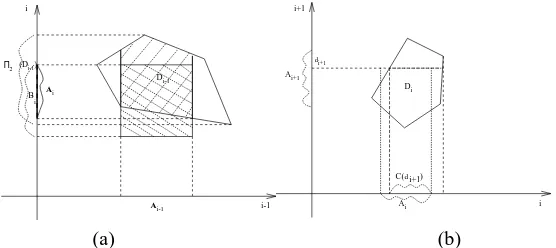
Now, in the forward sweep, as we may observe that for every parameter dieither the constraint domain coming from the segment(i−1,i), that is Di−1, or the one coming

from the segment(i,i+1), that is Di, have to be taken into account, we determine, for every parameter, the true admissible domain Ai. This is indeed done by algorithm A1.

Algorithm A1.

1. Set A0:=B0,J :=N

2. For i =1, . . . ,N

2.1 Set Ai :=52(Di−1∩ {Ai−1×Bi}). 2.2 If Ai = ∅set J :=i and stop.

3. Stop.

In this connection, we have the following result, [4].

THEOREM 1. P1 has a solution if, and only if, J = N that is Ai 6= ∅, i = 0,1, . . . ,N . If(d0,d1, . . . ,dN)is a solution then

(3) di ∈ Ai; i =0,1, . . . ,N.

We remark that, in general, a solution of P1 is not unique and that the necessary condition (3) is not sufficient. Thus, if the sequence of non empty sets A0, . . . ,AN has been defined by algorithm A1, a first simple scheme for computing a sequence (d0,d1, . . . ,dN)is provided by the following algorithm (backward sweep) whose ef-fectiveness is guaranteed by Theorem 2 (we refer again to [4] for the proof).

Algorithm A2.

1. Choose any dN ∈ AN . 2. For i =N−1,N−2, . . . ,0

2.1 set Ci(di+1):=51(Di∩ {Ai× {di+1}})

2.2 Choose any di ∈Ci(di+1)

(4)

THEOREM2. Let the sequence A0,A1, . . . ,AN be given by algorithm A1, with

Figure 1: Algorithm 1: construction of the admissible domains Ai,(a). Algorithm 2: graphical sketch of step 2.1.(b).

2.1. Boundary conditions

When we are constructing closed curves the end points should be handled as the other inner points so that the solution s(t)has to satisfy the condition s(k)(x0) = s(k)(xN) for k = 0,1, . . .up to the continuity order considered. This kind of conditions are called non separable boundary conditions. In terms of abstract scheme formalization the above conditions reduce to find a sequence(d0,d1, . . . ,dN)such that dN =β(d0),

whereβis any continuous function with continuous inverse.

These conditions, giving a direct relationship between the first and last element of the sequence(d0,d1, . . . ,dN), destroy the sequential structure of our scheme. A pos-sible strategy would consist in considering, among all the sequences(d0,d1, . . . ,dN) which belong to D, the ones where starting with an element d0 ∈ A0, end up with

(5)

2.2. Selecting an optimal solution

It is clear from algorithms A1 and A2 that it is possible to find infinite sequences (d0,d1, . . . ,dN) satisfying the constraints, as in algorithm A2 the admissible sets Ci(di+1), defined in step 2.1, do not reduce, in general, to a single point. It is therefore

a natural idea to look for an optimal sequence, where the optimality criterion can be given as the maximum or the minimum of a suitable functional F that is

(4) max

(d0,d1,...,dN)∈D

F(d0,d1, . . . ,dN) ,

and we specify the functional F according to our requirements. Although several forms of functionals could be considered, for the sake of simplicity, we shall limit ourselves to

where gigives the local contribution to the objective function and, in shape-preserving problems, can be connected with the shape of the resulting function (we shall consider the area bounded by a closed curve).

To solve the optimization problem we present here an approach based on dynamic programming (DP) [2]. As we will see later, this approach is well suited to deal with discrete problems. Moreover DP is extremely flexible, as many functionals and any kind of separable constraints (i.e. constraints which can be related to only one curve segment and then whic can be expressed separately from segment to segment) can be processed using the same algorithmic structure and, unlike other optimization meth-ods, constraints play here a positive role, limiting the size of the decision space. In this regard, we may observe that the functional recurrence relations of dynamic program-ming can be very efficiently linked with the constraints in Algorithm A2. We refer to [9] for full details on how implement dynamic programming in Algorithm A2.

Below is reported a sketch of the algorithm where we have stored in 8i the cost associated with the i -th stage and in Ti is stored the optimal policy (therefore

(6)

3. Compute dN such that8N(dN)= max

δN∈AN

8N(δN)

4. For i =N−1, . . . ,0 4.1. di :=Ti(di+1)

5. Stop.

2.3. Multivariate case

The two-sweep scheme, given by algorithms A1 and A2 (or A2DP), has turned out to be an effective method to solve several problems and its main attraction relies in the fact that it is general, being applicable to a wide range of problems.

However an its closer inspection shows us that, although there is no assumption on the subsets Di ofRq ×Rq, which are the basic elements of the imposed constraints, the practical usage of this method has been so far confined to the case Di ∈ R×R, that means q = 1. This is due to the fact that in algorithms, either A1 or A2 we have to compute the projection of intersections of subsets in a product space. More precisely, we may recall, for instance, that step 2.1 of A1, which is the kernel of all the modifications and improvements later developed, requires the computation of the following set:

Ai :=52(Di−1∩ {Ai−1×Bi}),

and this leads, even in the simplest higher dimension case, that is q=2, to intersections and projections of arbitrary subsets ofR2×R2. Even in the case of linear inequalities for the constraints (Di would be a polytope of R4), the corresponding algorithm is extremely difficult to implement and has an unaffordable computational cost. Indeed, inRq, the computational cost of set intersections and their projections is given by

O(nq−1log n), where n is the number of polytope vertices, see [15] for full details. Thus, the practical application of abstract schemes has been for many years re-stricted to univariate problems, where we have only one parameter associated with every knot (two for every segment). This limitation is rather restrictive as univariate problems suffice in general to model interpolation of functions, while are not suitable for interpolation of parametric curves, which can represent closed curves. We may see that usually parametric planar curve interpolation gives rise already to constraint domains inR2×R2.

Recent research has been therefore devoted to develop a new theory and construct new methods suitable and applicable to multivariate constraint problems (see for in-stance [7], [14]). It is worthwhile to repeat that the dimension q of the parameter space is not related to the dimension of the point space we are working in.

(7)

We refer to [9] for full details on this new approach. For the sake of completeness we report here the main ideas on how this approximation is performed.

For every domain Di, we suppose we are able to give an estimate of a lower and/or upper bound for each dimension. Then we may choose a step size h=(h1,h2, . . . ,hq) and, starting from the lower (upper) bound, construct a multidimensional grid inRq×

Rqwhose dimension is assigned. We thus approximate every domain Diwith the union of those boxes whose vertices are contained in Di. By construction we have Dei ⊆ Di and we may easily see that, given h, for h→0, we have meas(Di\Dei)→0.

The next step consists in making a further approximation. Once we have obtained the domains Dei, we consider only the discrete values for the parameters (di,di+1),

corresponding to the vertices of the considered boxes. This is equivalent to working with discrete domains, which we denote by Di. We then select the points of the grid which are vertices of a 2q-box contained in Di. At the end of this process we obtain a sequence of domains Di such that again approximate Diand Di ⊆Di.

As in the continuous case, we may select an optimal solution by optimizing a suit-able functional, using dynamic programming. The fact that the parameters di vary in discrete domains is well suited for applying the dynamic programming in the mini-mization process. Regarding the convergence analysis, the following result holds (we refer to [9] for the proof).

i i+1

D

i

h

i i+1

(a) (b)

Figure 2: (a):Every domain Di is replaced by a union of 2q-boxes.(b) only the values at the vertices of the considered boxes are taken.

THEOREM3. Let the domains D0,D1, . . . ,DN−1, with Di ⊂Rq×Rq, be given.

Let D0,D1, . . . ,DN−1 be the corresponding discrete domains obtained with a grid of step size h. Let us denote now with(d∗₀,d∗₁, . . . ,d∗_N)a solution in D which max-imizes also a continuous functional F, with a unique absolute maximum, and let (d¯∗₀,d¯∗₁, . . . ,d¯∗_N)be a discrete counterpart. Then

lim hmax→0(

¯

d∗₀,d¯∗₁, . . . ,d¯∗_N)=(d∗₀,d∗₁, . . . ,d∗_N) , hmax :=max(h1,h2, . . . ,hq) . We remark that as the parameters(di,di+1)can assume only the discrete values

(8)

logical operators AND, OR, taking only some planes, putting together more planes and so on. This way of proceeding has revealed to be very effective from the computational point of view and it can be extended straightforwardly to domains inRq ×_Rq _(the number of planes is in general given by 2q).

3. Interpolating spline curves maximizing the bounded area

Let us suppose we are given a set of points Ii ∈ R2, i = 0,1, . . . ,N , along with

a parameterization ti i = 0,1, . . . ,N , (for instance chord length). Let us indicate

with Li :=Ii+1−Ii the polygonal data and set the quantities ki :=ti+1−ti ,eLi := (Ii+1−Ii)/ki.

Our goal is to construct an interpolating C1spline curve, s(t), which bounds max-imal area. In order to obtain a curve useful for the applications we consider the addi-tional constraint of shape preservation, i.e. we require that the resulting curve preserves the convexity and inflections as prescribed by the given data.

To express the spline curve we use the piecewise B´ezier representation so that each spline segment is a B´ezier curve Bernstein polynomials of degree n, defined by Bn,j(u)=

From the properties of B´ezier splines we have that the resulting curve will be uniquely determined once the control polygon for every segment is constructed, see for instance [11]. By construction we have that b0,i =Ii and bn,i =Ii+1, in this way,

as B´ezier curves pass through the first and the last control points, we are guaranteed the resulting curve interpolates the given data.

Let us consider now curves of degree three. In this case, for each segment i , the control points to be determined are b0,i,b1,i,b2,i, and b3,i. The first and the last points are set equal to two interpolation data points. So we have to determine the two inner control points. From cubic B´ezier polynomial properties we have that the global curve is C1if and only if, for every segment i , the inner control points b1,iand b2,iare taken

where the vectors Ti and Ti+1, are respectively the curve tangent vectors at

interpola-tion points Iiand Ii+1.

If we express the tangent vectors as

(9)

where we set I−1=IN−1, t−1=tN−1, and IN+1=I1, tN+1=t1, the free parameters

to be determined in order to uniquely construct the resulting curve are the values of ui andvi, for every segment i =0, . . . ,N−1. These being two dimensional vectors, the problem is called bivariate.

It is a standard practice to express the shape-preserving conditions through the con-trol points. Indeed, due to the variation diminishing property of cubic B´ezier polyno-mials, a sufficient condition to locally reproduce the convexity of the polygonal data is that the corresponding control polygon is convex as well. This condition can be given by the following relationships

(8)

(eLi−1∧eLi)·((b1,i−Ii)∧(b2,i −b1,i)) ≥0 (eLi∧eLi+1)·((b2,i−b1,i)∧(Ii+1−b2,i))≥0.

We have to reformulate the shape-preserving conditions in terms of parameters

ui andvi. The resulting curve should belong to the portion plane between Li and the prolongations of Li−1 and Li+1; this can be assured imposing this condition to

the tangent vectors giving rise to the condition ui, vi ≥ 0. Moreover, a necessary condition for (8) (which can be easily deduced from the limit case of collinear data points) is given by

(9) 0≤ui ≤3, 0≤vi ≤3.

Let us then define the quantitiesρi := k(eLi−1∧eLi)kandσi := k(eLi−1∧eLi+1)k,

for i =0, . . . ,N . Using (7) the conditions (8) can be rewritten, after straightforward

computations, as

(10)

  

ui(3−ui+1)ρ_i2−uivi+1ρiσi−vivi+1ρiρi+1≥0 vi+1(3−vi)ρ_i2₊₁−uivi+1ρi+1σi −uiui+1ρiρi+1≥0 .

From the above expressions we get immediately the form of the constraints do-mains,

(11)

Di := { (ui, vi,ui+1, vi+1)∈R2×R2 such that

ui(3−ui+1)ρi2−uivi+1ρiσi−vivi+1ρiρi+1≥0; vi+1(3−vi)ρ2_i₊₁−uivi+1ρi+1σi−uiui+1ρiρi+1≥0; ui, vi,ui+1, vi+1 ≥ 0}.

3.1. Optimization process

Our goal is to select as optimal solution the one which maximize a suitable functional related to the area bounded by the curve (applying Algorithm A2DP).

(10)

polygonal line and the spline curve. As we consider interpolating spline curves the region bounded by the polygonal line is fixed, therefore we may restrict our attention to maximizing the area (which can be also negative) between the polygonal line and the curve.

The construction of the curve is done segment by segment (piecewisely), we may then maximize for each segment the area Si bounded by the curve s(t)for t∈[ti,ti+1]

and the line connecting Ii and Ii+1. Using polar coordinates we may see that the area Sican be expressed in the following way

(12) Si :=

where x(t)and y(t)are respectively the x and y components of the parametric curve

s(t). We should remark, that in this case the data points have to be ordered anti-clockwise. The global functional we maximize is then given by

(13) F(d0,d1, . . . ,dN):=

N_X−1

i=0 Si .

Regarding the error we make in the discretisation process, it can be proven the following result (for the proof we refer again to [8]).

THEOREM4. For every segment [i,i +1], let us define the discrete and the

con-tinuous optimal solutions respectively

where, the first one is computed using the discrete domains whose grid step size is h, then, setting hmax =max(h1,h2, . . . ,hq)and ki =ti+1−tiwe have

(14) k¯s∗_i(t)−s_i∗(t)k∞≤hmax

ki 4 .

4. C2Continuity

We consider now the problem of constructing spline curves with C2continuity. The idea is to start from a C1piecewise curve and modify it such that it still satisfies the imposed constraints, has maximal area, and it is also of the required continuity order along the pieces.

(11)

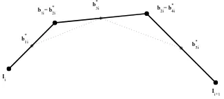
Let us consider the generic i -th interval. Taking the control polygon of the cu-bic B´ezier curve Ii,b1,i,b2,i,Ii+1 and inserting a collinear point in every

polygo-nal segment we obtain a control polygon with seven vertices, namely Ii,b∗₁_,_i,b∗₂_,_i =

b1,i,b∗₃_,_i,b∗₄_,_i = b2,i,b∗₅_,_i,Ii+1, corresponding to a B´ezier curve of degree six. By

construction, at each end point the curve has second derivative equal to zero, giving rise to a global C2spline curve. Moreover, as the shape of the control polygon is not changed the shape-preserving properties are maintained.

For the sake of simplicity the three additional points, b∗₁_,_i,b∗₃_,_i,b∗₅_,_i, can be taken as midpoints of each polygonal segment.

The C1continuity is guaranteed if we keep the points b∗₁_,_i and b∗₅_,_i fixed. On the other hand the requirement of C2continuitys¨i(ti+1)= ¨si+1(ti+1)can be rewritten in

terms of control points, taking into account that for curve of degree six we have (see for instance [11])

In order to maintain shape-preserving requirements the resulting control polygon should have the same convexity of the initial control polygon. More precisely the point b∗₂_,_ishould belong to the triangle whose vertices are b∗₁_,_i, b1,iand b∗₃_,_i, and equivalently

Figure 3: Starting control polygon for C2continuity.

(12)

approximate them with a union of hyperrectangles and take only the discrete values corresponding to the vertices.

Analogously to what we have done in the cubic case, we can now compute, for every segment i , the area bounded by the polygonal line and the curve and maximize it. This procedure lead to an optimal C2spline curve.

5. Numerical results

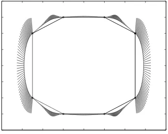
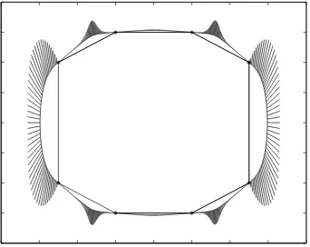
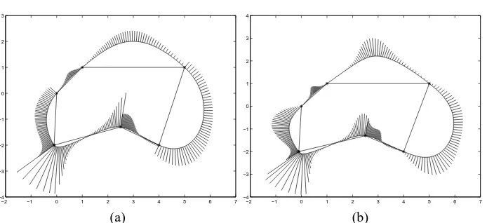
In this section we present the performance of the proposed scheme on three examples. In every case, in order to better comment the results obtained the curves will be depicted along with the curvature at the normal direction (porcupine representation),

The first example is about a symmetric set of data proposed the first time by Kaklis and Sapidis in [12]. The resulting curves are shown in Figures 4-5, where it is also displayed the polygonal line connecting the data. More precisely in Figure 4 it is shown the resulting C1shape-preserving curve which interpolates the given data, and maximize the bounded area.

Figure 4: C1cubic spline curve.

In Figure 5 the spline curve with C2continuity is shown where, again the result is obtained though the maximization of the bounded area. We may note numerically that in this case, having performed a second optimization process the total area is increased. The second example concerns a set of data taken from a ship hull. The results are displayed in Figure 6. Again we observe experimentally that the spline curve with

C2 continuity has a bounded area which is increased with respect to the area of the corresponding C1curve.

(13)

Figure 5: C2spline curve of degree 6.

(a) (b)

(14)

−2 −1 0 1 2 3 4 5 6 7 −4

−3 −2 −1 0 1 2 3

−2 −1 0 1 2 3 4 5 6 7

−4 −3 −2 −1 0 1 2 3 4

(a) (b)

Figure 7: Example 3:(a) resulting cubic spline curve with C1continuity.(b) resulting spline of degree six with C2continuity.

References

[1] ASATURYANS., COSTANTINIP. AND MANNIC., G2 Shape-preserving para-metric planar curve interpolation, in: “Designing and Creating Shape-Preserving

Curves and Surfaces”, (Eds. Nowacki H. and Kaklis P.), B.G. Teubner, Stuttgart 1998, 89–98.

[2] BELLMANR.ANDDREYFUSS., Applied dynamic programming, Princeton Uni-versity Press, New York 1962.

[3] COSTANTINIP., An algorithm for computing shape-preserving splines of

arbi-trary degree, Journal of Computational and Applied Mathematics, 22 (1988).

[4] COSTANTINIP., A general method for constrained curves with boundary

condi-tions, in: “Multivariate Approximation from CAGD to Wavelets”, (Eds. Jetter K.

and Utreras F.I.), World Scientific Publishing Co., Singapore 1993.

[5] COSTANTINIP., Abstract schemes for functional shape-preserving interpolation, in: “Advanced Course on FAIRSHAPE”, (Eds. Nowacki H. and Kaklis P.), B.G. Teubner, Stuttgart 1996, 185–199.

[6] COSTANTINIP., Boundary-valued shape-preserving interpolating splines, ACM Transactions on Mathematical Software 23 2 (1997), 229–251.

[7] COSTANTINIP.AND SAMPOLIM. L., Abstract schemes and constrained curve

interpolation, in: “Designing and Creating Shape-Preserving Curves and

Sur-faces”, (Eds. Nowacki H. and Kaklis P.), B.G. Teubner, Stuttgart 1998, 121–130. [8] COSTANTINIP.AND SAMPOLIM. L., A general scheme for shape preserving

(15)

[9] COSTANTINIP. AND SAMPOLI M. L., Constrained interpolation inR3 by ab-stract schemes, in: “Curve and surface design: Saint-Malo 2002”, (Eds. Lyche T.,

Mazure M.L. and Schumaker L.L.), Nashboro Press, Nashville 2003, 93–102. [10] GOODMAN T. N. T. AND UNSWORTH K., Shape preserving interpolation by

parametrically defined curves, SIAM J. Numer. Anal. 25 (1988), 1451–1465.

[11] HOSCHEK J.AND LASSERD., Fundamentals of computer aided geometric

de-sign, AK Peters Ltd., Wellesley 1993.

[12] KAKLISP. D. AND SAPIDISN. S., Convexity preserving polynomial splines of

non uniform degree, Computer Aided Geometric Design 12 (1995), 1–26.

[13] MULANSKYB.ANDSCHMIDTJ. W., Convex interval interpolation using

three-term staircase algorithm, Numerische Mathematik 82 (1999), 313–337.

[14] MULANSKY B. AND SCHMIDT J. W., Composition based staircase algorithm

and constrained interpolation with boundary conditions, Numerische

Mathe-matik 85 (2000), 387–408.

[15] PREPARATA F. P. AND SHAMOS M. I., Computational geometry,