Are School Finances Contributing
to Children’s Obesity?
Patricia M. Anderson
Kristin F. Butcher
a b s t r a c t
Over the last two decades the proportion of adolescents in the United States who are obese has nearly tripled, and schools, citing financial pressures, have given students greater access to “junk” foods, using the proceeds to fund school programs. We examine whether schools under financial pressure tend to adopt potentially unhealthful food policies and whether students’ Body Mass Index (BMI) is higher where they are more likely to be exposed to these food policies. We find that a 10 percentage point increase in poten-tial exposure to junk food in schools leads to about a 1 percent increase in students’ BMI.
I. Introduction
Over the past three decades, weight problems among children have grown dramatically. After holding fairly steady at around 5 percent during the 1970s, the percent of 12- to 19-year-olds who were obese doubled by the early 1990s and
Patricia Anderson is a professor of economics at Dartmouth College a researcher for the National Bureau of Economic Research and a coeditor of the JHR. Kristin Butcher is a researcher at the Federal Reserve Bank of Chicago. The authors thank Sara Christopher Champion, Karenne Eng, A. J. Felkey, Katharine Anderson, and Fred Yarger for excellent research assistance. Nancy Brener provided advice in using the SHPPS data. They also thank Lisa Barrow, David Card, Kevin Hallock, Helen Levy, Thomas Lemieux, Nina Pavcnik, Doug Staiger, and participants in presentations at UC-Berkeley, the Chicago Fed, the College of William and Mary, Dartmouth College, the NBER Summer Institute, and the University of Virginia for helpful discussions. The views expressed here are the authors’ and do not necessarily repre-sent those of the Federal Reserve Bank of Chicago, the Federal Reserve System, or any other entity. The authors take responsibility for all errors. A public-use version of the data used in this article can be obtained beginning January 2007 through December 2010 from Patricia Anderson, Department of Economics, Dartmouth College, Hanover, NH 03755-3514, patty.anderson@dartmouth.edu. [Submitted June 2004; accepted December 2005]
ISSN 022-166X E-ISSN 1548-8004 © 2006 by the Board of Regents of the University of Wisconsin System
The Journal of Human Resources 468
exceeded 15 percent by 2000 (Ogden et al. 2002).1At a basic physiological level, the
cause of this increase in overweight status among children is clear: Children must be taking in more energy than they expend. What is unclear is what has upset the bal-ance between energy intake and expenditure.
Observers have begun to question the role played by schools, pointing in particular to declines in physical education and increases in the availability of soft drinks and snack foods. New accountability measures, which typically require that students achieve a certain minimum level on standardized tests or the school suffers conse-quences, give schools an added incentive to invest resources in core academic curric-ula and cut back on electives. At the same time, schools may try to raise new money in order to meet the achievement goals while minimizing the need to cut noncore pro-grams. However, the property tax reform movement during the 1970s and 1980s lim-ited schools’ ability to raise money through traditional means. One way schools can get extra money to maintain optional programs or strengthen core academics is through soft drink and vending contracts, or through other snack food sales. The media is rife with examples of schools cutting deals with soda and snack vending companies in order to increase their discretionary funds. For example, one high school in Beltsville, Md. made $72,438.53 in the 1999-2000 school year through a contract with a soft drink company and another $26,227.49 through a contract with a snack vending company. The almost $100,000 obtained was used for a variety of activities, including instructional uses such as purchasing computers, as well as extracurricular uses such as the yearbook, clubs, and field trips (Nakamura 2001). District-level contracts can be even more lucrative—one Colorado Springs district, for example, negotiated a ten-year beverage contract for $11.1 million dollars (DD Marketing 2003).2
As school districts nationwide debate the benefits and costs of entering into contracts with soda companies or banning the sales or advertising of snacks and sodas on campus it is important to have solid information on which to base these decisions. For example, high-calorie snack foods and beverages may be so ubiquitous that adolescents will consume them whether or not they are available through the school. If that is the case, policymakers might prefer schools to sell the foods students crave. In that way, at least students are not leaving school (with all the dangers that may entail) to buy snack food and schools can use the extra funds to students’ advantage.
Thus, examining the effect of school food policies on children’s weight problems is important. However, it is difficult because no one data set contains information on children’s height and weight, along with individual and family characteristics that may affect weight problems and school food policies. Except for the school policies, the National Longitudinal Survey of Youth 1997 (NSLY97) contains all of the necessary information for a sample of adolescents. To use these data to address the question at
1. “Obese” here is defined as a Body Mass Index (BMI) above an age-sex specific cutoff defined by the Centers for Disease control. This cutoff corresponds closely to a BMI above the 95thpercentile of age-sex specific BMI distributions from the late 1960s and early 1970s prior to the advent of the current weight prob-lems in children.
hand, we just need to obtain a proxy for exposure to junk food and/or beverages in school. We take advantage of the fundraising potential of school food policies to cre-ate this proxy via a two-step procedure. In the first step, we examine whether avail-ability and advertising of snack foods and beverages in schools are related to school financial pressures, as captured by tax and expenditure limits, school accountability measures, state school financing rules, and relative growth in the school-aged (local) population. In the second step, we use this estimated relationship to predict exposure to these school food policies for adolescents in the NSLY97, and then examine whether availability and advertising of snack foods and beverages in schools can be linked to adolescent Body Mass Index (BMI).3
We find that there is a positive and often significant effect of predicted availability and advertising of snack foods and beverages on adolescent BMI. However, this rela-tionship is driven by those with an overweight parent. We interpret our results to indi-cate that while for most students school food policies have no affect on their weight, for those with a family susceptibility to weight gain, these policies that increase access to snack foods and beverages in school may be a contributing factor.
The paper is organized as follows. Section II provides background on the issues of school food policies and obesity in the United States. Section III describes our empir-ical approach and discusses our main estimates of the relationship between school food policies and finances and of the effect of school food policies on adolescent obe-sity. This section also discusses some alternatives to our preferred estimates. Section IV then explores the interaction of school food policy and family susceptibility to weight problems, and Section V concludes.
II. Background on School Food Policies and Obesity in
the United States
Public health officials are alarmed at the increase in obesity in the United States. The increase in childhood obesity is particularly worrisome as obesity in childhood has both immediate and long-term health risks, including Type 2 dia-betes, hypertension, and cardiovascular disease (Ebbeling, Pawlak, and Ludwig 2002), as well as contributing to low quality of life scores (Schwimmer, Burwinkle, and Varnie 2003). Using data from the National Health and Nutrition Examination Surveys (NHANES), Anderson, Butcher, and Levine (2003a) show that for both chil-dren and adults, the BMI distributions for 1971–74 and 1976–80 are very similar, par-ticularly in the right tail of the distribution. However, beginning with the 1988–94 NHANES, this right tail gets thicker.4The obesity “epidemic” does not appear to be
a matter of a shift to the right of the entire distribution of BMI. Rather, the
distribu-3. Body mass index is weight in kilograms divided by height in meters squared.
The Journal of Human Resources 470
tions suggest that whatever changes have taken place to upset the balance between energy in-take and energy expenditure have not affected everyone in the same way. There appears to be some fraction of the population that is particularly susceptible to obesity, and the current environment is particularly conducive to their condition.
It is in this setting that school food policies are currently being hotly debated. Policymakers are acting on the intuitive notion that having snacks and sodas readily accessible in schools contributes to children’s obesity.5Despite movements on the
legal and policy fronts, there are very few studies that address whether there is a direct relationship between school food policies and obesity.6What is clear, however, is the
pervasiveness of snack foods and beverages in U.S. schools. Data from the School Health Policies and Programs Study (SHPPS) from 1994 and 2000 form a nationally representative sample of schools, and include both public and private schools. As shown in Anderson, Butcher, and Levine (2003a), these data reveal two clear patterns. First, availability of food and sodas from vending machines increases with grade level. While only 27 percent of elementary schools had vending machines available to students in 2000, that percentage rises to 67 percent for middle schools and to 96 percent for high schools. Second, in the few questions asked consistently across the two years, food availability has increased. For example, while 19 percent of high schools served a brand name fast food in 1994, 26 percent did by 2000.
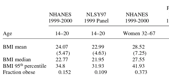
Before examining the effect of school food policies on children’s weight, we first present measures of BMI and obesity from the NHANES for comparison with the NLSY97 data used in our study. BMI for individuals in the NLSY97 is constructed from self-reported height and weight, while the NHANES includes an examination module where height and weight are measured. In Table 1 we report mean, median, and 95th percentile BMI for the NLSY97 analysis sample and for the subsample of similarly aged (14- to 20-year-old) respondents in the NHANES (1999-2000). Since we control for parental BMI in the analysis below, we also report BMI for parents in the NLSY97 and for similarly aged (32- to 67-year-old) adults in the NHANES.
Columns 1 and 2 in Table 1 show measures of BMI for adolescents. Mean and median BMI are both slightly higher in the NHANES, where height and weight are measured by an examiner, than in the NLSY97, where height and weight are self-reported. However, BMI at the 95th percentile is about 35 in the NHANES and only about 32 in the NLSY97. This translates into about 4 percent more of the adolescents in the NHANES categorized as obese than in the NLSY97 sample. The data for adults show a similar pattern. Both comparisons suggest that very heavy people are under-reporting their weight in the self-reported data, such that the self-reported data are prone to some measurement error.7Note that this measurement error affects BMI,
5. For example, New York City public schools recently banned candy, soda, and other sugary snacks from school vending machines (Perez-Pena 2003). Similarly, the Los Angeles school district has banned the sale of soft drinks during school hours (Fried and Nestle 2002).
6. Studies on related topics include Ludwig, Peterson, and Gortmaker (2001), Cullen et al. (2000), and Kubik et al. (2003) who examine school food and overall nutrition. In addition, Pateman et al. (1995) and Weschler et al. (2001) examine the availability of junk food in schools. Finally, Carter (2002) and Fried and Nestle (2002) spec-ulate about the correlation between school policies and adolescent obesity, but do not formally investigate the relationship.
which we use as a lefthand-side variable in our estimation. Measurement error in the lefthand-side variable will not bias our results unless it is systematically correlated with the first-step variables used to create our exposure proxy. As discussed further below there does not appear to be any correlation.
III. Effect of School Food Policies
on Adolescent Obesity
A. Methodology
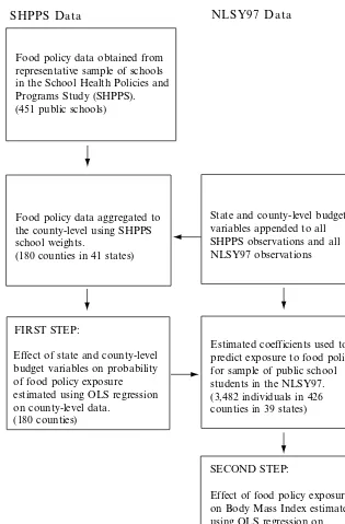
Figure 1 provides an overview of our empirical strategy, much of which is dictated by the realities of the data at our disposal. As mentioned, no available data sets include school policies regarding junk food, measures of school financial pressure, and indi-vidual heights, weights, and demographics. Ideally, if we had data with all of the ele-ments described above, we could directly investigate the relationship between school policies and student obesity. However, in this case one might be concerned about bias due to the possible endogeneity of the key food policy variables such that we would want to investigate the need for an instrumental variables approach. Because of this fact, it is tempting to think of our two-step approach as similar to two-sample IV (for example, Angrist and Krueger 1992 and 1995), but our approach uses an auxiliary regression to predict exposure to a food policy, which is unobservable in the data. Thus, it is actually a two-step model of the type discussed in Murphy and Topel
Table 1
Comparison of BMI and Obesity Across Data Sets
Parent’s of
NHANES NLSY97 NHANES NLSY97
1999-2000 1999 Panel 1999-2000 1999 Panel
Age 14–20 14–20 Women 32–67 32–67
BMI mean 24.07 22.99 28.52 26.53
(5.47) (4.63) (7.25) (5.87)
BMI median 22.77 21.95 27.55 25.10
BMI 95thpercentile 34.8 31.93 41.93 37.76
Fraction obese 0.152 0.109 0.373 0.228
(0.359) (0.312) (0.484) (0.419)
Sample size 1,742 3,482 1,293 3,482
The Journal of Human Resources 472
SHPPS Data
Food policy data obtained from representative sample of schools in the School Health Policies and Programs Study (SHPPS). (451 public schools)
Food policy data aggregated to the county-level using SHPPS school weights.
(180 counties in 41 states)
Effect of state and county-level budget variables on probability of food policy exposure estimated using OLS regression on county-level data.
(180 counties) FIRST STEP:
SECOND STEP:
Effect of food policy exposure on Body Mass Index estimated using OLS regression on individual-level data. (3,482 individuals)
Estimated coefficients used to predict exposure to food policy for sample of public school students in the NLSY97. (3,482 individuals in 426 counties in 39 states)
State and county-level budget variables appended to all SHPPS observations and all NLSY97 observations
NLSY97 Data
Figure 1
(1985), and we will calculate our standard errors accordingly. That said, because our two-step method uses exogenous state and county variables to predict the food policy proxy variable, it will address the endogeneity problem that would arise from using OLS with complete data.8
We use school food policy information from the representative sample of public schools surveyed in the SHPPS to create our proxy variable. Specifically, we try three different policies: junk food availability in schools, whether schools have “pouring rights” contracts, and whether soda and snack food advertisements are allowed at schools or school events.9None of these measures is clearly the best. They are
sim-ply different possible ways to capture exposure to unhealthful food in school. That said, “junk food” is likely the most broad measure, although it does not capture the availability of sugary beverages. Soda vending machines appear almost universal in high schools, though, making it unlikely that we could estimate an effect of soda availability with this method. Thus, in terms of sugary beverages, we consider the type of contract a school has and whether it allows advertising, rather than simple availability, to examine effects on adolescent weight.
We aggregate these measures of school food policy to the county level using the SHPPS school weights, where we have 451 public middle and high schools with non-missing information for our measures of school food policy. Our first step, then, esti-mates the fraction of schools in a county with these policies as a function of county, state, and regional characteristics.10 The county characteristics we use to predict
school food policies include the growth rate of the school age population relative to total population in the county, calculated from the 1990 and 2000 U.S. Censuses.11
Next, we control for the fraction of school finances that come from the state, calcu-lated from the National Center for Education Statistics (NCES) Common Core data. The NCES provides this information at the district level and we use district enroll-ments to aggregate to the county level. The state characteristics include an indicator variable for whether the state has a tax or expenditure limitation and an indicator for whether the state has passed a school accountability measure.12We also include a
vec-tor of three region dummies, R(the excluded category is the West).
8. As discussed further below, for a subsample of the data, we can directly match the county-level policy data with the individual data. OLS appears to be, if anything, negatively biased—students exposed to junk food are less likely to be overweight, all else equal. The true IV point-estimates are then very close to those obtained using the two-step method with these data. However, the two-step method sacrifices efficiency, resulting in larger standard errors. See Table A2.
9. See the appendixes for more details. “Junk Food Available” means that students can buy chocolate, candy, cakes, ice cream, or salty snacks (that are not fat free) from a machine or school store. “Pouring Rights” con-tract means the school has agreed to sell one brand of soft drinks, often in exchange for a percentage of sales or other incentive packages. “Soda or Snack Food Advertisements” means that advertisements are allowed at least at one type of school related activity or in one or more places at the school—for example, on a school bus, at a school sporting event, on school grounds, or school textbooks etc.
10. In about 10 percent of the counties in the SHPPS, we have data for only one school, while in another 20 percent, we have data on just two schools.
11. Specifically, this is defined for the county as the logarithm of the 5- to 17-year-old population in 2000 minus the logarithm of the 5- to 17-year-old population in 1990, all divided by the logarithm of total popu-lation in 2000 minus the logarithm of total popupopu-lation in 1990.
The Journal of Human Resources 474
Specifically, we estimate the following:
(1) policyc= γ0+ γ1relative school-age population growth ratec+ γ2fraction
of revenues from statec+ γ3tax limitations+ γ4accountabilitys
+ γ5Rs+ ωc
where the csubscript represents county and the ssubscript represents state.13
The relative growth in the school-age population is meant to capture budgetary pressure on the school system, thus we expect γ1to be positive. If the share of
chil-dren has grown relative to the share of adults, then there should be more financial pressure on schools, and they may be more likely to adopt these food policies that generate discretionary funds. Similarly, we expect γ4to be positive, because schools
in states with accountability laws are under pressure to meet certain performance cri-teria. These criteria generally take the form of standardized tests scores (not measures of students’ physical health), and thus schools may divert resources toward core aca-demics and away from other programs. In order to preserve optional programs, schools may then come up with creative ways to raise additional funds, including sales of snack foods and beverages.
The tax and expenditure limit indicator and the fraction of school revenues that come from the state are both meant to capture how difficult it is for schools to raise additional funds for valued programs. It will be more difficult for schools to raise funds through traditional means in a state with strict tax and expenditure limits, thus we expect γ3to be positive. We also expect it to be difficult to raise local funds if it is
typical for larger amounts of school funding to come from the state. Thus, we expect
γ2to be positive. Each state has a funding formula that specifies how much of a school
district’s funds will come from the state.14For this reason, we prefer to rely mainly on
the variation at the state level.15That is, we are comparing different systems, rather
than focusing on different treatments within a system. Within a state this fraction tends to be negatively related to fiscal capacity, and thus potentially to individual socioeconomic status. Across states, more school funding coming from the state may reflect more difficulty for local school districts to unilaterally decide to raise funds. This difficulty may simply be political—that is the district relies more on the state because it is difficult to pass higher local property tax rates. Alternatively, the diffi-culty may stem from characteristics of the local tax base. For example, localities with a large commercial base may be in a better position to raise funds because the busi-nesses pay local taxes, but do not increase the number of children requiring education. Finally, we control for region of the country (R) in both the first and second step to control for additional factors that may influence school food policy decisions and chil-dren’s obesity.
13. Later in the section we’ll investigate alternatives, such as including state fixed effects or a measure of socioeconomic status.
14. The most common approach is the foundation program, but other methods include a flat grant, percent-age equalizing, guaranteed tax base or guaranteed equal yield programs (Sielke and Holmes).
Having obtained estimates of γ0, γ1, γ2, γ3, γ4, and γ5 using the SHPSS/NCES/
Census county-level data, we then use these estimates to predict food policies in indi-vidual-level data from the NLSY97. Because the independent variables in the first step vary only at the county and state level, and since we know the county of residence for the NLSY97, we can append the appropriate fiscal, legal, and population change variables to the individual data and create predicted food policies based on the first–step estimates. This prediction can then serve as our proxy for exposure to unhealthful food in school, and we can then estimate the effect of food policy on indi-vidual weight status, controlling for additional covariates.
To do so, we use a model of the following form:
(2) ln (bmi)i= α + β1predicted policyc+ β2Xi+ β3Fi+ β4Ri+ εi
where ln(bmi)is the log of the individual’s Body Mass Index; Xis a set of individual-level covariates, including age, race, sex, and cigarette use; Fis a set of family back-ground covariates, including family income, mother’s and father’s education, and the log of the responding parent’s BMI; and Ris a set of region dummies. Finally, we adjust the standard errors for arbitrary forms of heteroskedasticity and within county correlation. In addition, in order to adjust for the fact that the food policy is estimated, we calculate the standard errors following Murphy and Topel (1985). In brief, all of the standard errors are adjusted by adding a term that depends on both the variance-covariance matrix from the first step and the second-step parameter on the estimated food policy variable.16For the key variable in our main model, the result is a standard
error that is about 20 percent higher than would be obtained from OLS.
B. The Relationship between School Food Policies and Finances
The results from the first step, in which we estimate Equation 1, are shown in Table 2. The first column gives the means of the independent variables while the first row gives the means for the dependent variables across the 180 counties represented in the SHPPS. First, note that all of the estimated effects for the models in this step are of the predicted sign. Because higher values for each independent variable represent a higher level of local budgetary pressure, our hypothesis predicts a positive coefficient. For both junk food and pouring rights, the fraction of total revenues that come from the state is significantly positive. For both junk food and school advertising, the tax and expenditure limit indicator is significant. Thus, at least one of the variables is sig-nificant in each case. The overall F-statistics and F-statistics for just those variables excluded from the second step are reported at the bottom of the table. They indicate that the overall models are highly significant in each case, and that the excluded vari-ables are jointly significant at better than the 1 percent level for both junk food and pouring rights, but are not significant at conventional levels for school advertising. Note that the standard errors are corrected for arbitrary forms of heteroskedasticity and within state correlation.17
16. See Equation 15’ in Murphy and Topel (1985).
Table 2
Step One Predictions of Food Policies
Fraction of Fraction of Fraction of
Mean of Schools in Schools in Schools in
Independent County in County with County
Variable which can “Pouring that allow
(Standard Purchase Rights” Food Ads
Deviation) Junk Food Contracts at School
Mean of dependent
Variable (standard 0.748 0.671 0.441
deviation) (0.352) (0.405) (0.406)
Share of total revenue 0.495 0.350 0.502 0.371
from state sources (0.142) (0.157) (0.239) (0.241)
State has tax and 0.472 0.113 0.077 0.119
expenditure limits (0.501) (0.061 (0.059) (0.061)
1990 to 2000 relative 0.939 0.0003 −0.0004 0.0020
growth rate in county (10.18) (0.0016) (0.0025) (0.0020)
population aged 5–17
State has school 0.856 0.070 0.113 −0.042
accountability rules (0.353) (0.100) (0.073) (0.102)
Northeast 0.156 0.102 −0.061 −0.102
(0.363) (0.089) (0.139) (0.122)
Midwest 0.261 −0.156 0.212 0.130
(0.440) (0.068) (0.071) (0.095)
South 0.372 0.047 0.140 0.233
(0.485) (0.071) (0.075) (0.077)
Constant 0.469 0.193 0.131
(0.121) (0.151) (0.167)
Sample size 180 180 179 180
R-squared 0.1334 0.1058 0.1344
Overall F-statistic 10.07 5.20 5.23
p-value for overall 0.0000 0.0003 0.0003
F-test
F-statistic for excluded 3.88 4.91 2.04
variables
p-value for excluded 0.0094 0.0026 0.1069
variables F-test
C. The Effect of Predicted School Policies on Obesity
The results from estimating Equation 2 described above are reported in Table 3. Columns 1 and 2 use junk food availability as the predicted policy, Columns 3 and 4 use pouring rights, and Columns 5 and 6 use soda or snack food ads. Recall that while each is a potential proxy for exposure to unhealthy food and beverages in school, junk food is likely to be the broadest measure and we focus mainly on it. For each policy, the first model includes no covariates other than region dummies, while the second estimates Equation 2 in full. The first thing to note is that the additional covariates have very little impact on the key policy coefficient. This result is not really unex-pected, given that the policy variable is predicted based on exogenous fiscal policy measures that are unlikely to be highly correlated with the individual’s demographic background.18
Focusing on the results that include the full set of controls, the Column 2 estimates imply that a 10 percentage point increase in the proportion of schools in a county that make junk food available to their students is correlated with a nearly 1 percent (0.90 percent) increase in students’ BMI. The results are smaller for the fraction of schools with pouring rights contracts, and marginally significant. The results for the fraction of schools that allow advertising are smaller still and are insignificant. This result suggests that it is the actual availability of potentially unhealthful foods that affects adolescents’ weight, as opposed to the type of contract the schools sign with soda pur-veyors or the advertising they allow.
Turning to the estimates for the other variables, the point estimates imply that females and those from richer families have lower BMIs, while blacks and Hispanics have higher BMIs.19Perhaps the most interesting control variable is the parental BMI,
which implies an elasticity of 0.22 between child and parent.20This strong correlation
provides evidence on the importance of shared genetics, shared environment, or both.
D. Alternative Specifications
The evidence to this point is strongly suggestive of a role in adolescent weight prob-lems for the availability of junk food through schools. It is important to realize, though, that budgetary pressures are likely to result in a range of school actions beyond increased food and beverage sales. To the extent that these sales are highly correlated with other things affecting student health, such as cutting physical educa-tion, we cannot separately identify the effects.21Given the lack of ideal data, the
mod-18. The fact that the results do not change a great deal when we include individual measures of socioeco-nomic status suggests that variation in our measures of school food policies is not driven by unmeasured dif-ferences in socioeconomic status. Below we investigate the role of socioeconomic status more fully. 19. Note that in the NHANES females are not less likely to be obese, so our finding may be a reflection of sex-specific errors in the NLSY97 self-reported height and weight.
20. Note that 83 percent of the time this parent is the biological mother, while 11 percent of the time it is the biological father. Another 3 percent are a related female guardians and the rest are mainly stepmothers. If we limit the sample to only those for whom the responding parent is the biological mother, we get nearly identical results.
The Journal of Human Resources
478
Table 3
Estimated Effect of Predicted School Food Policies on Ln(BMI) Public School Students in the NLSY 1997
Policy: Policy: Policy: Policy: Policy: Policy: Beverage
Junk Food Junk Food Pouring Pouring Beverage or or Snack
Available Available Rights Rights Snack Food Ads. Food Ads.
(1) (2) (3) (4) (5) (6)
Predicted 0.106 0.090 0.099 0.075 0.041 0.038
Policy (0.052) (0.045) (0.052) (0.042) (0.041) (0.033)
African 0.034 0.035 0.034
American (0.012) (0.012) (0.012)
Hispanic 0.016 0.017 0.016
(0.011) (0.011) (0.011)
Female −0.027 −0.027 −0.027
(0.007) (0.007) (0.007)
Age 0.019 0.019 0.019
(0.003) (0.003) (0.003)
Family income −0.015 −0.014 −0.014
(in 100,000s) (0.009) (0.009) (0.009)
Ln(parent’s BMI) 0.221 0.221 0.221
(0.018) (0.018) (0.018)
Sample size 3,482 3,482 3,482 3,482 3,482 3,482
R-square 0.0037 0.1078 0.0040 0.1074 0.0022 0.1065
Mean (standard deviation) 0.758 0.759 0.684 0.684 0.438 0.438
of predicted policy (0.119) (0.119) (0.137) (0.137) (0.168) (0.168)
Mean (standard deviation) 3.117 3.117 3.117 3.117 3.117 3.117
of dependent variable (0.183) (0.183) (0.183) (0.183) (0.183) (0.183)
els estimated here can never be definitive. However, we can explore several potential areas of concern in hopes of adding weight to the validity of our results.
First, one might be concerned that there are characteristics of individuals or places that affect BMI that are correlated with our predicted school food policy vari-ables. For example, one might be concerned that socioeconomic status (SES), which research shows is correlated with obesity, is also correlated with our pre-dicted food policy. While we include a rich set of individual-level controls for SES it is possible to add an aggregate measure of SES in both steps. We investigate three such measures computed at the county level: per capita income, percent black and percent college graduate. Only per capita income is significant (and then only at the 9 percent level) in predicting junk food availability. Interestingly, this significant effect on junk food availability is positive. Thus, contrary to what one might have assumed, higher SES communities are more likely to make junk food available in schools. In the second step estimation, per capita income is negative and insignifi-cant, while the effect of junk food drops slightly to 0.062. With a standard error of 0.038, this point estimate is neither significantly different from our preferred esti-mate in Table 3 nor from zero.
One may still be concerned that unobserved variables resulting in spurious correla-tion are driving our results. Presumably, any such spurious correlacorrela-tion would apply to both student’s BMI and their parent’s BMI. However, any true impact of food policies in school should affect only the students, not their parents. Thus, as a falsification exercise we use the parental BMI as the dependent variable in the second step.22The
coefficient (standard error) on junk food in this specification is −0.018 (0.045), which is significantly different from the result for students, and not significantly different from zero.23Thus, it does not appear that our main results are driven by some simple
form of spurious correlation due to unobservables.
Another concern is that our state-level variables are really only capturing fixed state effects. In order to see whether our state variables are merely picking up across state differences, we estimated a set of “placebo” results where we estimated the first step with only a full set of state dummies, but excluded these from the second step. If this had given us similar results to those reported in Table 3, we would have been con-cerned that our predicting variables were working through unobserved state differ-ences, as opposed to through the budgetary pressures posited above. However, we find no effect of the food policy variables when predicted from state fixed effects.
One might also worry, though, that state fixed effects belong in both the first and second step (in other words, that there are unobserved characteristics at the state level that drive both food policies and adolescent BMI). Because much of the variation in our policy variables is at the state level via differences in accountability and tax and expenditure limitations, we allow only for region, rather than state fixed effects. Nonetheless, if we replace our region dummies with state dummies (and thus drop the
or administrators per student, the instruments are all of the expected sign, but are not jointly significant. Thus, there is no significant effect in the second step.
22. We drop the student-specific covariates of age, sex, and smoking behavior, but add student BMI to pro-vide for the role of genetics.
two state-level variables), the effect of junk food drops slightly (in this case to 0.074) but again is not significantly different from our preferred estimate. Precision is lost, however, as the two remaining excluded variables are only jointly significant at the 6 percent level in the first step.
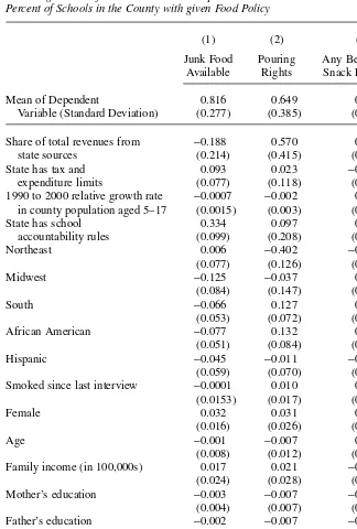
Finally, for a nonrandom subset of the data, we can match the county-level policy from the SHPPS data to the individual-level data from the NLSY97.24There are 1,007
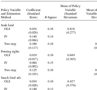
individuals, living in 78 different counties for whom we can perform this match. As a check on our two-step procedure, we estimate several models with these matched data. First, we estimate Equation 2 using OLS, where “predicted policy” is no longer predicted, but is the actual fraction of sampled SHPPS schools in the county report-ing the policy. We then estimate the same model by IV, usreport-ing the state and county legal, finance, and population change variables from Equation 1 as the excluded instruments. In addition, we then use the two-step procedure on the smaller matched sample and compare these results with the IV results. The first-stage results are reported in Table A1. The OLS, IV, and two-step results are reported in Table A2.
The point estimates from the two-step and IV models are very similar to each other, and to those in Table 3. However, the smaller sample size results in relatively large standard errors, such that none are significant at conventional levels.25For junk food,
recall that in Table 3 the estimated effect was 0.090, with a standard error of 0.045. The IV model in the matched sample produces an estimated effect of 0.140, but with a standard error of 0.084. Standard errors are even larger with the two-step method. The matched sample two-step procedure yields a slightly larger estimate of 0.160, with a standard error of 0.117. Based on the matched sample, we conclude that our two-step method is producing estimates similar to what would be obtained from a standard IV model, but that we pay a price with slightly larger standard errors.
A perhaps more interesting comparison is that between the OLS and IV estimates for the matched sample. The OLS point estimates are uniformly smaller (between 0.019 and 0.034) than the IV or two-step estimates, and not significantly different from zero. The implication, then, is that the OLS estimates are biased downward. One possibility is that the types of areas with more junk food, pouring rights contracts, and snack food ads are the types of areas for which other unobservables would tend to pro-duce leaner adolescents.26For example, suppose that parental demand for better
aca-demic achievement, more extracurricular activities (or both) is behind schools raising additional funds through food policies. These same demanding parents may provide more healthful foods and exercise opportunities in their homes than less involved par-ents, resulting in a negative bias in the OLS estimates. This possibility is supported by the earlier finding that junk food availability seems to be positively correlated with SES. Alternatively, simple attenuation bias due to measurement error in the policy variable may explain the larger IV estimates.
The Journal of Human Resources 480
24. Data Appendix Table 1 shows summary statistics for all the variables in the overall and matched sam-ples of the NLSY97. The means are very similar for the two samsam-ples, especially for BMI. The main differ-ences seem to be that there are more respondents in the West and fewer in the South in the matched sample. 25. Recall there are only 78 counties represented in these matched data, greatly reducing the variation used to estimate the policies.
Overall, then, it appears that while our two-step procedure can only ever be sug-gestive of the positive effect on adolescent BMI of the availability of junk food through schools, many potential problems can be ruled out. In addition, the value of the two-step procedure as a method to deal with endogeneity in food policy is appar-ent, but perhaps not in the manner expected. It appears that schools in better-off com-munities are more likely to offer junk food to their students. Thus, even though food and beverage availability can be predicted by budgetary pressures, it is not the low SES areas that turn to food and beverage sales to raise money.
IV. The Interaction of School Food Policy and Genetics
(or Family Susceptibility)
The overall results can be summarized as implying that a 10 percentage point increase in the proportion of schools with junk food is correlated with about a 1 percent higher BMI for the average student. There are smaller and often insignificant effects for the other food policies examined here. One should not read the estimates in Table 3, however, as implying that every student exposed to such food policies will increase their BMI by 1 percent. A fairly large literature exists documenting a strong genetic component to weight (for example, Grilo and Pogue-Geile 1991). At the same time, the increases in obesity over the past 20 years clearly cannot be attributed to changes in the gene pool. Thus, it seems reasonable to expect that some portion of the population has a genetic susceptibility for weight gain, and under certain conditions will, in fact, be more likely to gain weight. The idea of a genetic predisposition for weight gain is at the heart of the theory of the “thrifty gene” by pioneering geneticist James Neel (Neel 1962). In studying the Pima Indians, he theorized that in difficult times, when many Pima died of starvation, the survivors had a genetic advantage in stor-ing energy as fat. This “thrifty gene” was then passed on to future generations. In mod-ern times, when the Pima live in an environment of relative caloric abundance, this genetic predisposition toward more efficient fat storage results in high rates of obesity.
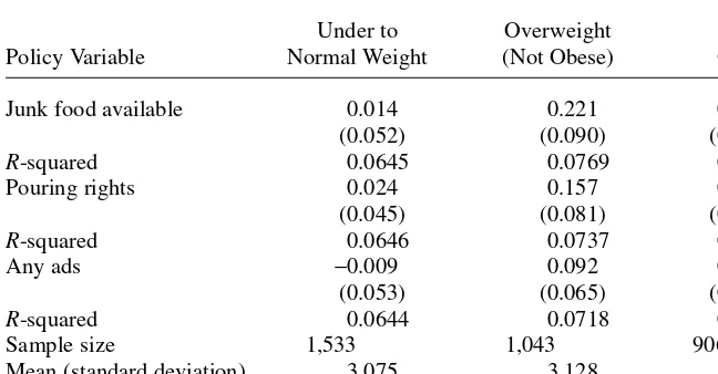
It is with this idea of the interaction between nature and nurture in mind that we estimate Equation 2 separately by parental weight status. Table 4 shows results sepa-rately for those whose responding parent is normal weight (BMI<25), overweight (25<=BMI <30), and obese (BMI>=30). For completeness we show the results for
all the policies, although only those for junk food availability are significantly differ-ent from zero. While it is difficult to get precise estimates for these smaller subgroups, the effect of junk food on adolescents whose parents are overweight is statistically significantly different from those whose parents are normal weight.27For the students
with a normal weight parent, there is essentially no effect of junk food (or any of the other policies) on their BMI. However, for those whose parent is overweight, a ten percentage point increase in the proportion of schools with junk food availability increases their BMI by more than 2 percent (2.21 percent). For those whose parent is obese, the effect is not different from either other subgroup. As noted in the appen-dix, though, there is a good deal of measurement error in parental BMI, the most
The Journal of Human Resources 482
likely result of which is for those with normal weight parents to be misclassified as having an underweight or obese parent. Because we group the underweight with the normal weight, the main impact will be on the obese group. Thus, the lack of a larger effect for the obese parent group may just be due to misclassification. Alternatively, it may be the case that children of obese parents are doomed to weight gain, no mat-ter what happens in the schools. Such a result could be true either with a very strong genetic component or simply a high-calorie household environment.
The estimates for the effect of pouring rights contracts and advertisements are less pre-cise than for junk food. However, in each case, the point estimates for those with over-weight parents are much larger than for those with normal and under over-weight parents. Thus, there is evidence that for those who are genetically susceptible to weight gain, the school environment may play an important role. At the same time, for the 44 percent of students with normal weight parents, the school food policy makes no difference at all.
V. Summary and Avenues for Future Research
Researchers and public health officials are currently at a loss to explain the rapid rise in weight problems among children and adolescents. Although
Table 4
Estimated Effect of Predicted School Food Policies on Ln(BMI) Public School Students in the NLSY 1997 by Responding Parent’s Weight Status
Under to Overweight
Policy Variable Normal Weight (Not Obese) Obese
Junk food available 0.014 0.221 0.079
(0.052) (0.090) (0.110)
R-squared 0.0645 0.0769 0.0360
Pouring rights 0.024 0.157 0.076
(0.045) (0.081) (0.098)
R-squared 0.0646 0.0737 0.0361
Any ads −0.009 0.092 0.0004
(0.053) (0.065) (0.049)
R-squared 0.0644 0.0718 0.0351
Sample size 1,533 1,043 906
Mean (standard deviation) 3.075 3.128 3.194
of dependent variable (0.154) (0.180) (0.212)
Notes: See notes to Table 3 for information on the data and estimation method. All models include the same set of controls variables as Columns 2, 4, and 6 in Table 3. The standard errors (in parentheses unless noted otherwise) are corrected both for arbitrary correlation within county, and for the fact that the policy variable is estimated. Under to normal weight is defined as a BMI<25, overweight (not obese) is defined as a
it is clear that weight gain is attributable to taking in more energy than one expends, it is unclear what has upset the balance between energy intake and expenditure in recent decades. Thus, it is important to consider the environmental factors that may affect either the intake or expenditure of energy. In looking at adult obesity, Cutler, Glaeser, and Shapiro (2003) point to technological innovations over recent decades that have lowered the time cost of food consumption. The result of these lower time costs is increased caloric intake. In the adolescent context, the increasing number of schools that allow students access to junk food or provide vending machines for stu-dent use might be considered examples of this type of technological innovation.
Perhaps not surprisingly, then, policymakers have begun to point to school food poli-cies as potentially important contributors to student weight problems. Although no solid evidence currently exists on this link, several large school districts have banned or severely restricted the availability of sodas and snack foods in schools. This paper takes a first step at assessing the effect of school food policies on adolescent weight.
We find that schools that are under financial pressure (as captured by our available data) are more likely to make junk food available to their students, have pouring rights contracts, and allow food and beverage advertising to students. We use measures that capture financial pressure to predict the fraction of schools in a county with these par-ticular food policies, and then estimate the effect of the fraction of schools in a county with these food policies on adolescent BMI. First, this two-step method is the only way to examine this question because there are no data with information on students’ BMI and their schools’ food policies. Second, however, this method is meant to give us variation in school food policies that is correlated with schools’ fiscal capacity, but not directly correlated with unobservable factors linked to the prevalence of unhealthy weights among the students.
We find fairly robust evidence that an increase in the proportion of schools making junk food available to students is linked to an increase in students’ BMI. Our results for the other school policies, pouring rights contracts, and food and beverage adver-tisements are smaller and less precise. The results suggest that a ten point increase in the percentage of schools in a county that allows its students access to junk food leads to a 1 percent increase in students’ BMI. Because average weight for adolescents in this sample is about 148 pounds, this translates into about 1.5 extra pounds per 10 per-centage point increase in availability.
Currently, policymakers are acting to reduce access to junk food and soda in a number of school districts around the country, with the express purpose of curbing adolescent obesity. We can do a rough “back of the envelope calculation” to bound how much of the recent increase in adolescent BMI may be attributed to the increased availability of such foods in schools over the last decade.28Data from the 1994 and
2000 waves of the SHPPS show that the percentage of high schools giving their stu-dents access to vending machines increased from 88 percent to 96 percent, or by eight percentage points. Unfortunately, the 1994 SHPPS data do not allow us to calculate the fraction of schools giving access to junk food, and “junk food availability” and “access to a vending machine” are not the same thing.29Junk food may be available
through cafeterias and school stores, for example, and vending machines may stock healthful snacks. Thus, for this rough calculation, we assume that the increasein access to junk food is the same as the increase in access to vending machines. Our estimates for the impact of junk food availability on adolescent BMI imply that an eight percentage point increase in the number of schools allowing students access to junk food would translate into about a 0.8 percent increase in BMI on average. Data from the NHANES show that BMI among 12- to 19-year-olds increased by about 3.5 percent between the 1988–94 and the 1999–2000 interviews. Roughly then, about a fifth (22 percent) of the average increase in adolescent BMI could be attributed to the increase in availability of junk food in schools.30
Thus, policymakers may be disappointed if they are expecting reductions in junk food availability in schools, for example, to be a “magic bullet” in the fight against adolescent obesity. Future research might fruitfully examine the impact of these changes on the ground in New York and Los Angeles and other school districts where they have banned certain junk foods. Evaluations of the impact will need to consider which products are allowed to substitute for soda and junk foods (for example, fruit juices, which are allowed under most of these revised school policies, often have just as many calories as nondiet soda). In addition, evaluators should take into account the benefits of existing school food policies. If it is the case that existing food policies help generate funds for valuable pro-grams, then the benefit (potentially to all students) needs to be weighed against the health costs borne by the fraction of students with a susceptibility to obesity.
Data Appendix
Because no one data set contains all of the variables necessary for our analysis, we must build our data from several different sources. These include the School Health Policies and Programs Study (SHPPS), the Common Core of Data for school districts from the National Center for Education Statistics (NCES), county The Journal of Human Resources
484
28. This calculation uses the authors’ calculations from the NHANES and SHPPS data reported in Anderson, Butcher, and Levine (2003a) Tables 1 and 6.
29. In particular, only about 75 percent of schools give students access to foods we have defined as “junk food” in 2000, while 96 percent give students access to a vending machine.
Table A1
First Stage Results for the “Matched” Sample
Percent of Schools in the County with given Food Policy
(1) (2) (3)
Junk Food Pouring Any Beverage or
Available Rights Snack Food Ads
Mean of Dependent 0.816 0.649 0.427
Variable (Standard Deviation) (0.277) (0.385) (0.376)
Share of total revenues from −0.188 0.570 0.311
state sources (0.214) (0.415) (0.377)
State has tax and 0.093 0.023 −0.045
expenditure limits (0.077) (0.118) (0.094)
1990 to 2000 relative growth rate −0.0007 −0.002 0.002
in county population aged 5–17 (0.0015) (0.003) (0.001)
State has school 0.334 0.097 0.381
accountability rules (0.099) (0.208) (0.138)
Northeast 0.006 −0.402 −0.460
(0.077) (0.126) (0.120)
Midwest −0.125 −0.037 0.063
(0.084) (0.147) (0.160)
South −0.066 0.127 0.159
(0.053) (0.072) (0.074)
African American −0.077 0.132 0.015
(0.051) (0.084) (0.049)
Hispanic −0.045 −0.011 −0.153
(0.059) (0.070) (0.049)
Smoked since last interview −0.0001 0.010 0.017
(0.0153) (0.017) (0.021)
Female 0.032 0.031 0.022
(0.016) (0.026) (0.023)
Age −0.001 −0.007 0.014
(0.008) (0.012) (0.011)
Family income (in 100,000s) 0.017 0.021 −0.051
(0.024) (0.028) (0.031)
Mother’s education −0.003 −0.007 −0.007
(0.004) (0.007) (0.004)
Father’s education −0.002 −0.007 −0.002
(0.003) (0.006) (0.005)
Ln(parent’s BMI) 0.001 −0.001 0.023
(0.034) (0.060) (0.047)
Sample size 1,007 1,007 1,007
population data from the 1990 and 2000 Census, and individual-level data on public school students from the National Longitudinal Survey of Youth 1997 (NLSY97). We describe our use of each of these in turn.
The SHPPS is a national study conducted in 1994 and 2000 for the Center for Disease Controls (CDC).31While the study covers a broad range of school health policies and
procedures at the state, district, school and classroom level, we focus on the 2000 school environment survey. This questionnaire asks about the school’s policies regarding such things as the availability of snack foods through vending machines, school stores and snack bars; the details of an exclusive contract with a soft drink manufacturer (if any); and the types of advertising for sodas and snack foods allowed. Unfortunately, the major-ity of these questions were not asked in 1994. While unlike the 1994 study, the 2000 study also includes elementary schools, we do not include them in our main analysis, since we will be focusing on youths aged 14 and older who are enrolled in public schools. We choose three food policies from the SHPPS for the bulk of our analysis. First is an indicator of student access to junk foods, defined as the availability through vend-ing machines or school stores of chocolate candy; other candy; cookies, crackers, cakes, pastries or other baked goods that are not low in fat; or salty snacks that are not low in fat. Second is an indicator for having an exclusive “pouring rights” contract with a soft drink manufacturer. Third is an indicator that advertisements promoting student consumption of candy, meals from fast food restaurants or soft drinks are per-mitted in any number of ways, such as in the school building, on textbook covers or food service menus, on buses, or at athletic fields.
Because we are focusing on public school financing issues, we limit ourselves to the public schools in the SHPPS. We use data on the 451 public middle and high schools for which all the variables we need have nonmissing information. For these schools we can identify their school district and merge on district-level information about school finances from the NCES Common Core of Data.32The SHPPS data give
The Journal of Human Resources 486
31. For more information on SHPPS, see http://www.cdc.gov/nccdphp/dash/shpps/.
32. More information about the NCES Common Core of Data can be found at http://nces.ed.gov/ccd/.The latest fiscal data available at the time the project began were for the 1998-99 school year. Thus, the fiscal data lags the policy data by one year.
Table A1 (continued)
(1) (2) (3)
Junk Food Pouring Any Beverage or
Available Rights Snack Food Ads
F-statistic for excluded 10.87 1.74 6.14
instruments
p-value for excluded instruments 0.0000 0.1709 0.0012
the QED (Quality Education Data) district codes. We purchased the cross-walk between the QED and NCES district codes from QED. We use the NCES district codes to merge data on district finance information from the NCES. While detailed financial data is available, we want a simple summary measure of local fiscal capacity. Thus, we choose to use the fraction of total district revenues that come from the state, since even state funding formulas that are not explicitly equalization schemes, such as the most common foundation grant formula, result in there being a negative correla-tion between local fiscal capacity and the state share of funding.33
33. See, for example, the summary discussion of Public School Finance Programs in the United States and Canadaby Sielke and Holmes at http://www.ed.sc.edu/aefa/reports/ch1.pdf.
Table A2
Estimated Effect of Food Policy on Ln(BMI)
OLS, IV and Two-Step Estimation with the “Matched” Sample
Mean of Policy
Policy Variable Coefficient Variable Mean of Predicted
and Estimation (Standard (Standard Variable (Standard
Method Error) R-Square Deviation) Deviation)
Junk food
OLS 0.034 0.16 0.816
(0.028) (0.277)
IV 0.140 0.14
(0.084)
Two-step 0.160 0.16 0.758
(0.117) (0.128)
Pouring rights
OLS 0.019 0.16 0.649
(0.017) (0.385)
IV 0.084 0.15
(0.092)
Two-step 0.125 0.16 0.650
(0.103) (0.124)
Snack food ads
OLS 0.034 0.16 0.427
(0.026) (0.376)
IV 0.146 0.13
(0.070)
Two-step 0.139 0.16 0.410
(0.135) (0.146)
The Journal of Human Resources 488
The lowest geographic level of detail available in our individual-level data sets is the county. We therefore aggregate the SHPPS and NCES data up to the county level.34Using the school weights in the SHPPS, then, we calculate the probability that
a school in the county has each of these policies. There are 180 counties in 41 states covered in our SHPPS sample. The NCES fiscal data is averaged across all districts in the county using district enrollment levels as weights. Finally, we merge on two state-level indicators and the county-level relative growth in the school-age popula-tion. The first indicator is for whether the state has tax and expenditure limitations in place.35These types of local limits were commonly passed beginning in the late 1970s
and into the 1980s, with some states tightening their laws in the early 1990s. The sec-ond indicator is for whether a state has passed a school accountability measure.36
These types of laws are mainly of a much more recent vintage, with many not imple-mented until the mid-1990s. Data Table A3 provides a complete list of states with each of these types of laws and the dates they were implemented. Finally, we compute the relative growth rate for the school-age population based on county-level popula-tion figures for those aged 5–17 and the total populapopula-tion from the 1990 and 2000 Census. The growth rate is then calculated as:
Ln(aged 5–17 population in 2000) -Ln(aged 5–17 population in 1990) divided by Ln(total population in 2000) -Ln(total population in 2000).
Table 2 includes the sample means of each of these predictor variables.
The second major component of the project uses individual level data on adolescents that includes height and weight, along with individual and family background demo-graphics. The National Longitudinal Survey of Youth, 1997 panel (NLSY97) is a sur-vey of 8,984 youths who were aged 12–16 as of December 31, 1996. The first round of the survey took place between February of 1997 and May of 1998. Additional waves have been carried out annually during the school year. We use data from Wave 3, which was collected in the 1999–2000 school year, to be in accord with the SHPPS data.
Wave 3 of the data contains information on 7,958 individuals. We limit that to those who are enrolled in public school, which reduces the sample to 4,653 individuals. By the time we eliminate those with missing information for variables used in our analy-sis, we are left with a working sample of 3,482 individuals. In order to use our two step estimation, we append the data on state tax limitations and state accountability laws to the NLSY97 data using state identifiers provided in the confidential geocode data. Similarly, we append county level data on the share of total school revenue from state sources, and the 1990 to 2000 relative growth rate in the county population aged 5–17 using the county identifiers in the geocode data. The individuals in our NLSY97 sample live in 426 counties.
We measure the adolescents’ weight status using the log of their body mass index (BMI). BMI is defined as weight in kilograms divided by height in meters squared (kg/m2) and is a commonly used measure to define obesity and overweight in adults.
For example, according to guidelines in National Institutes of Health (1998), adults are considered underweight if their BMI is less than 18.5, overweight if their BMI is 25 or more, and obese if their BMI is 30 or more. Use of the BMI to assess
Full Sample Matched Sample
The Journal of Human Resources 490
dren and adolescents has been slightly more controversial, although its use is fairly widespread.37The Centers for Disease Control (CDC) has recently endorsed the use
of BMI to assess overweight status in children and adolescents, and has produced sex-specific BMI distributions for children aged between two and 20 for just this purpose. While results are similar using probability of overweight, we choose to use the con-tinuous BMI measure.
Before calculating BMI, however, we make a few corrections for obvious typo-graphical problems with the recorded height and weight data. As a first step in clean-ing the weight data, we replace any weight value in a given year with the average from the years surrounding it if the given value is less than half or more than double the average of those surrounding it. So for example, for a Wave 3 weight observation, we replace it with the average of the Wave 2 and Wave 4 weight values if it is less than half or more than double the average of the Wave 2 and 4 values.
Because several individuals are missing weight data for one or more years, this presents a problem in comparing a given weight value to the values surrounding it. So, we employ an additional screening method. We flag weight values less than 60 or greater than 300 and then examine them by hand to distinguish between those individuals who have consistently high or consistently low weights and those indi-viduals who have a single weight value which is very different from all other avail-able weight data for that individual. For those individuals who have an outlier weight value, we replace it with the average of the weight values from the closest waves.
After creating the BMI values, we then flag any value less than 10 or greater than 40. We chose 10 and 40 as our cutoff values because the third percentile for a 12-year-old is around 15 and the 97th percentile for a 20-year-12-year-old is 35. For those individuals with a flagged BMI, we then examine the height values by hand in order to identify those height values which clearly stand out from the rest. In all cases, only the feet value of height is altered since it is virtually impossible to determine if the inches values are inaccurate. The outlier height values are replaced with the nearest height value that makes sense. For example, an individual with the height values 5’10”, 8’11”, 5’11”, 5’11”, 6’0” will have the 8’ replaced with 5’. An individual with the height values 4’11”, 7’2”, 5’2”, 5’3”, 5’3” will have the 7’ replaced with 5’. Finally, the BMI values are recomputed using the altered weights and altered heights. Ultimately, only five sample BMI values are different from those computed from the recorded values.
We also use parental BMI in the analysis. This information was collected in the initial wave from the responding parent (88 percent are biological mothers, 10 percent are bio-logical fathers, 3 percent are related female guardians, and 2 percent are stepmothers).
Data Table A4
Tax and Expenditure Limits and School Accountability By State
Tax and Year of Year
Expenditure Enactment, School System
State Limits Tightening Accountability Implemented
Alabama No Yes 1997
Alaska No No
Arizona Yes 1975, 1990 Yes 2000
Arkansas Yes 1982 Yes 1999
California Yes 1978 Yes 1999
Colorado Yes 1974, 1990 Yes 1999
Connecticut No Yes 1984
Delaware No Yes 1998
District of Columbia No Yes 1997
Florida No Yes 1999
Georgia No Yes 2000
Hawaii No No
Idaho No No
Illinois No No
Indiana Yes 1974 Yes 1995
Iowa Yes 1972, 1992 No
Kansas Yes 1974 Yes 1995
Kentucky Yes 1980 Yes 1995
Louisiana Yes 1979 Yes 1999
Maine No Yes 1999
Maryland No Yes 1999
Massachusetts Yes 1981 Yes 1998
Michigan Yes 1979 Yes 1998
Minnesota Yes 1972 Yes 1996
Mississippi Yes 1984 Yes 1994
Missouri Yes 1981 Yes 1997
Montana Yes Yes 1998
Nebraska No No
Nevada No Yes 1996
New Hampshire No Yes 1993
New Jersey Yes 1977 Yes 1995
New Mexico Yes 1980 No
New York No Yes 1998
North Carolina No Yes 1993
North Dakota No No
Ohio Yes 1977 Yes 1998
Oklahoma No Yes 1996
Oregon Yes 1991 Yes 2000
The Journal of Human Resources 492
There are outliers in these data as well, but with only one year of information, we cannot follow the procedure described above for identifying incorrect information. Bad data leading to the misidentification of students as having “obese” parents may explain why our results for that subgroup are relatively imprecise. Without other information, our options for dealing with misreported data are limited. We reestimated the results in Table 3 dropping those with parents with BMIs above 40, above 50, and above 60. These three sets of results are very similar to those in Table 3.
One other key explanatory variable needs some recoding. We want to control for an individual’s socioeconomic background, so we construct a variable that will capture each individual’s permanent household income. Because the youth in our sample are all enrolled in public schools, in most cases this variable is the average of the gross household income values of a youth’s parents over the period 1996–2000 (collected in 1997–2001). For 1996, we use a gross household income variable that was constructed using information collected during the initial parent interview.38For 1997
through 2000, we use gross household income variables constructed using informa-tion from household income update quesinforma-tionnaires. The household income update questionnaires were administered each survey year to the parents of individuals who still lived at home. They collected the following information:
38. In a few cases (2 percent of the full sample), youth who were considered independent answered these income questions instead of the parent.
Data Table A4 (continued)
Tax and Year of Year
Expenditure Enactment, School System
State Limits Tightening Accountability Implemented
Rhode Island No Yes 1997
South Carolina Yes 1981 Yes 1999
South Dakota No No
Tennessee No Yes 1996
Texas Yes 1983 Yes 1994
Utah No No
Vermont No Yes 1999
Virginia No Yes 1998
Washington Yes 1980 Yes 1998
West Virginia No Yes 1997
Wisconsin No Yes 1993
Wyoming No Yes 1999
● whether the parent had an income
● the amount of the parent’s income if it existed
● whether the parent’s spouse/partner had an income
● whether the parent and spouse/partner had any other forms of income
● the amount of the other income if it existed
The gross household income variables we use for 1997 through 2000 are created so that income from a particular source is zero if the parent responding reports that they did not have that type of income, is the amount of that type of income if the amount is available and the parent reports that they do have that type of income, and is missing otherwise. The income amounts from each of the three distinct sources are then summed to get a gross household income variable for 1997–2000. For these years, if the gross household income value is still missing after using the household income update information, we replace it with a household income value collected from each youth aged 14 and older in the 1998–2001 surveys.39We then convert each of these final gross household income
variables to 2000 dollars. Finally, in order to get a variable representative of “permanent” household income, we average gross household income across all years, 1997–2001. We replace this permanent household income value with a missing value if we do not have at least two years of valid household income data to calculate the average.
References
Anderson, Patricia M., Kristin F. Butcher and Phillip B. Levine. 2003a. “Economic Perspectives on Childhood Obesity.” Federal Reserve Bank of Chicago Economic Perspectives21(3):30–48.
Anderson, Patricia M., Kristin F. Butcher and Phillip B. Levine. 2003b. “Maternal Employment and Overweight Children.” Journal of Health Economics22(3):477–504. Angrist, Joshua, and Alan Krueger. 1992. “The Effect of Age at School Entry on Educational
Attainment: An Application of Instrumental Variables with Moments from Two Samples.” Journal of the American Statistical Association87(418):328–36.
———. 1995. “Split-Sample Instrumental Variables Estimates of the Return to Schooling.” Journal of Business and Economic Statistics13(2):225–35.
Carter, Robert Colin. 2002. “The Impact of Public Schools on Childhood Obesity.” Medical Student Journal of the American Medical Association288:2180.
Cawley, John. 1999. “Rational Addiction, the Consumption of Calories, and Body Weight.” Dissertation. University of Chicago.
Cullen, Karen Weber, Jill Eagan, Tom Baranowski, Emiel Owens, and Carl de Moor. 2000. “Effect of a la Carte and Snack Bar Foods at School on Children’s Lunchtime Intake of Fruits and Vegetables.” Journal of the American Dietetic Association 100(12):1482–86.
Cutler, David M., Edward L. Glaeser, and Jesse M. Shapiro. 2003. “Why Have Americans Become More Obese?” Journal of Economic Perspectives17(3):93–118.