Manajemen | Fakultas Ekonomi Universitas Maritim Raja Ali Haji 516.full

(1)

All- Cause Mortality Reductions from

Measles Catchup Campaigns in Africa

Ariel BenYishay

Keith Kranker

BenYishay and Kranker

abstract

As recently as 1999, 13 million measles cases and 500,000 measles- related deaths occurred in sub- Saharan Africa per year. Over the past decade, vaccination coverage across the continent has improved dramatically, largely as a result of the Measles Initiative, an international effort coordinating and funding national mass- immunization campaigns. We estimate the reduction in all- cause child mortality after initial countrywide measles vaccination campaigns using variation in the timing of the campaigns across countries and subnational regions. This framework accounts for competing and complementary risks as well as for contemporaneous trends in mortality rates that may have biased case- based estimates. We use birth and death history data compiled from multiple Demographic and Health Surveys for 25 countries and control for country- speciﬁ c trends in child mortality and time- varying factors that were associated with campaign timing. Our ﬁ ndings show that the Measles Initiative campaigns raised the probability of a child’s survival to 60 months by approximately 2.4 percentage points for cohorts treated by the campaign. The campaigns cost approximately $109 per child life saved, remarkably low in absolute terms as well as relative to other interventions to reduce global child mortality.

I. Introduction

Historically, measles was one of the most lethal infectious agents, responsible for _fi ve to eight million annual deaths globally prior to 1963 (Moss and Ariel BenYishay is Assistant Professor of Economics at the College of William & Mary. Keith Kranker is an economist at Mathematica Policy Research. They thank Abhijeet Anand, Athalia Christie, Denise Doiron, Dominick Esposito, Matt Ferrari, Jane Fortson, Mark Grabowsky, Jack Molyneaux, Lorenzo Moreno, Maya Vijayaraghavan, seminar participants at the University of Colorado- Denver and the University of New South Wales, and three anonymous referees for providing helpful comments. Algerlynn Gill provided excellent research assistance. They thank Mathematica for allowing access to servers. All errors are their own. The views herein are those of the authors and do not necessarily refl ect the views of their affi liated institutions. This article uses data from the Demographic & Health Surveys (DHS), which may be available by request via the DHS site [http://dhsprogram.com/data/available-datasets.cfm]. The authors are willing to advise other scholars about access and compilation of this data. Other data used in the study are avail-able from the authors beginning November 2015 through October 2018.

[Submitted February 2013; accepted April 2014]

(2)

BenYishay and Kranker 517

Scott 2009). The disease, which is often contracted in regular epidemic outbreaks, sup-presses the immune system of infected individuals—primarily children—weakening their defense against complications from diseases such as acute encephalitis, diarrhea, and pneumonia (Moss and Scott 2009; Ferrari et al. 2008). The licensure of the measles vaccine in 1963 and its subsequent use throughout the developed world induced by 1987 a precipitous drop in global measles deaths to 1.9 million (Wolfson et al. 2007).

In sub- Saharan Africa, though, coverage lagged signi_ﬁ cantly in the _ﬁ rst 35 years after the vaccine’s licensure: By 2000, routine coverage of the measles vaccine on the con-tinent stood at only 56 percent. As a result, 337,000 measles- related deaths occurred in Africa in 2000—about half of worldwide childhood deaths due to vaccine- preventable diseases (Simons et al. 2012; Wolfson et al. 2007; Stein et al. 2003).

Although routine vaccination coverage has remained low in sub- Saharan Africa, a new phase in strategic coordination of measles vaccination efforts has yielded dramatic improvements. These efforts, under the Measles Initiative (MI) program, involved sup-plementary immunization activities (SIAs), or “catchup campaigns,” that cover nearly all of the child population in a targeted country. They are complemented by (1) subsequent followup campaigns and (2) capacity building to improve routine coverage, surveillance, and clinical management of measles patients (Wolfson et al. 2007). As of 2010, the MI had coordinated SIAs in 31 African countries. Because they generally reached more than 90 percent of the target population (the mean SIA coverage rate in our sample is 97 percent), these SIAs raised the population vaccination coverage rate dramatically. Table A1 in the supplementary appendix1_{details the routine vaccination coverage prior to the} ﬁ rst SIAs in our sample and the number of children vaccinated in each SIA.

The burden of the disease prior to these efforts and the scale of these coverage improvements merit a rigorous assessment of the MI’s mortality and morbidity effects, particularly in light of recent funding cuts (Strebel et al. 2011). Unfortunately, weak surveillance systems lead to severe underreporting of measles cases in sub- Saharan Africa (with case- detection rates of 5 percent to 40 percent, at best), and reporting of measles- related deaths to WHO is limited (Wolfson et al. 2007) and omits measles’ impact on other causes of death (Walker et al. 2013). Nonetheless, reported measles cases decreased by 67 percent in sub- Saharan Africa between 2000 and 2010 (based on 2010 WHO data), although this value may understate the true percentage reduction in cases (Wolfson et al. 2007). Estimates of the true reduction in cases reach as high as 90 percent (Measles Initiative 2011). Such a dramatic reduction in observed measles cases warrants a careful estimation of the associated reduction in all- cause mortality.

Without reliable surveillance data on cases and outcomes, researchers have looked to epidemiological models to estimate the effects of measles SIAs on mortality (McLean and Anderson 1988; Miller 2000; Henao- Restrepo et al. 2003; Stein et al. 2003; Otten et al. 2005; Wolfson et al. 2007; Simons et al. 2012). However, existing epidemiological mod-els rely on problematic data and strong assumptions. First, the modmod-els are based on sur-veillance data with high and variable underreporting although increasingly sophisticated methods are addressing this challenge (see Simons et al. 2012). The basic strategy of us-ing measles case- reportus-ing data to predict mortality is controversial (Saurabh and Kumar 2012). Second, the estimates of case- fatality ratios (CFRs) on which the models rely have been shown to be highly uncertain (Lim et al. 2008; Wolfson et al. 2009, pp. 2–3). Third,

(3)

The Journal of Human Resources 518

these models hold country- speci_fi c CFRs constant over time, despite evidence of _fl uctua-tions and trends in CFRs. Notably, CFRs vary over time based on changes in economic development, health system improvements, nutrition, HIV/AIDS, Vitamin A supplements, and vaccination itself (Barclay, Foster, and Sommer 1987; Helfand et al. 2005). Trends in CFRs can explain large historical decreases in measles mortality (McKeown 1979, p. 105) in a period where more than 90 percent of children contracted measles before their 15th birthday (Strebel et al. 2011, p. 1). Fourth, the relationship between measles- related deaths and all- cause mortality depends on the extent of competing and complementary risks. A recent systematic review by Walker et al. (2013) compared cause- speci_fi c and all- cause mortality reductions from pre- MI interventions, _fi nding a large indirect effect of measles vaccination on diarrhea deaths. This is consistent with clinical observations of measles indicating suppression of the immune system of infected individuals, weakening their defense against complications from diseases such as diarrhea, acute encephalitis, and pneumonia (Cutts 1993; Ferrariet al. 2008). However, such effects are not included in the aforementioned epidemiological models. Finally, the models do not account for contemporaneous factors (including other government and donor efforts) that may affect measles incidence, measles mortality, and competing or complementary risks.

This study provides the _ﬁ rst estimates of the impact of the MI catchup campaigns using survey- based mortality data and an identi_ﬁ cation strategy that accounts for trends in mortality rates over the same time period. That is, we directly measure the effect of the campaigns on all- cause mortality instead of using a modeling- based ap-proach. The staggered timing of the campaigns by country across the continent allows us to identify the impact of a campaign by comparing the mortality rate in countries where campaigns took place relatively early with those where they occurred relatively later while controlling for trends over time in these countries’ overall mortality rate. That is, we use difference- in- differences methods, common in economics literature (Imbens and Wooldridge 2009, p. 67), and apply this approach in the context of a survival model. We use the continent- wide coverage of the Demographic and Health Surveys (DHS), which include maternal interviews that provide complete birth and child death histories, to estimate the impact of the SIAs on all- cause mortality.

This identi_fi cation strategy is similar to those of several other recent papers that study the mortality reductions from large- scale antimalarial interventions (Bleakley 2010; Cutler et al. 2010) and a working paper on the effect of India’s Universal Immu-nization Program (Kumar 2011). This paper is the _fi rst to use data from a wide panel of countries (accounting for a majority of sub- Saharan Africa’s population) and to es-timate treatment effects shortly after their occurrence. Relatively few studies combine DHS data from multiple survey countries for econometric impact analysis (examples include Fortson 2009, 2011; Case and Paxson 2011); our study is the _fi rst to do so in the context of a large- scale program evaluation across Africa.

II. Empirical Approach

(4)

data are currently available. Campaigns in these countries were conducted between September 2001 and December 2007. We exclude countries without campaigns on the grounds that they do not offer a valid counterfactual.2

The MI campaigns involved several innovative features. Preparation for the cam-paigns involved staff organization and training on injection safety and post- campaign case surveillance, as well as the provision of new equipment for maintaining the cold chain where needed (Otten et al. 2005; Levine 2007). In addition, because measles is highly contagious, vaccination coverage rates over 90 percent are needed to achieve herd immunity (Christie and Gay 2011; Wolfson et al. 2007). The campaigns therefore aimed to reach this threshold quickly (typically within one to two weeks). To do so, the campaigns relied on community- based mobilization activities, including information dissemination to mothers and caretakers through local volunteers and awareness- raising in primary schools (Levine 2007). The sharp timing allows identi_ﬁ cation of the effects of the campaign while controlling for gradual changes in local child mortality rates.

According to American Red Cross (ARC) staff responsible for campaign planning, cam-paign timing was driven by political stability and public security, readiness of the country’s Red Cross/Red Crescent society and health ministry for participation in the campaign, and region- speci_fi c seasonality in measles incidence. We control for these factors with country- speci_fi c dummies and time trends, plus related time- varying covariates capturing political stability, security, health sector capacity, and region- speci_fi c seasonality. After controlling for these factors, we argue that remaining variation in the timing of the cam-paigns is exogenous to the factors driving measles cases and mortality rates and thus al-lows empirical identi_fi cation of the causal impact of the campaigns on childhood mortality. This study’s empirical approach is feasible because the MI campaigns covered entire countries (or large portions of countries) within a very short time frame (typically one to two weeks), and the DHS surveys provide nationally representative child mortality data. Measles outbreaks are episodic at a local level (Ferrari et al. 2008; Ferrari, Djibo, Grais, Bharti et al. 2010; Ferrari, Djibo, Grais, Grenfell et al. 2010). Thus, it would be virtu-ally impossible to detect changes in measles mortality immediately after a campaign in small geographic units (say, cities or districts within each country). However, as Ferrari et al. (2008, pp. 679–80) notes, the erratic and synchronous local epidemics aggregate to annual cycles in measles mortality when using data at a national scale, making possible the detection of effects over annual or biannual intervals. Again, we control for seasonal cyclicality and, in some models, region- speci_fi c seasonal cyclicality.

Our identi_ﬁ cation strategy exploits differences in the timing of the campaigns across countries and, in some cases, across regions within countries. For example, a child born in Niger in January 2000 might have received the vaccine at 59 months old, but a child born in Tanzania would have been vaccinated at 21 months. We can thus compare the mortality risk of similarly aged children and attribute the difference to the differential timing of the MI campaign.

2. In several of these campaigns, additional interventions were administered alongside the measles vaccina-tions. These were Vitamin A drops, polio vaccinations, and/or deworming medicavaccina-tions.

(5)

Our empirical strategy also accounts for the fact that the MI may have different ef-fects for older and younger children, all else equal. Two factors are at play. First, older and younger children were exposed to the disease (that is, not vaccinated) for different lengths of time: Children born a longer time before the campaign had more time to become infected simply because they were older when the MI campaign occurred in their campaign- region. The second factor is that we expect declining mortality risk from measles as children age. Although the campaigns targeted all children between the ages of nine months and 15 years (in some instances, the upper bound was 14 years), we focus on under- _ﬁ ve mortality because the mortality risk from measles is dramatically higher among younger children. In particular, we would expect declines in mortality to be concentrated in the younger cohorts. Wolfson et al.’s (2009, pp. 199–200) metastudy shows that measles CFRs among children aged less than 36 months was 15 percent or higher, but the measles CFRs were not signi_ﬁ cantly different from zero for children aged 36 months or older. (According to MI staff, the campaigns vaccinated older children primarily to reduce the likelihood of transmitting the disease to younger children.) It is also worth noting that child mortality rates are highest for young children (that is, a 1 percent reduction in one- year- old mortality rates would avert more deaths than a 1 percent reduction in three- year- old mortality rates).

We use two distinct estimation approaches to consider the effects of these differences: (1) a child- level regression model that assesses the effect of the campaign on children’s survival until age _ﬁ ve, and (2) a duration model that permits us to test whether changes in mortality rates occur contemporaneously with MI campaigns. The child- level model provides an estimate that combines the two effects (exposure duration and differential mor-tality risks) while the duration model only estimates the latter (by holding exposure periods constant). Sections IV and V discuss the details of these models and compare the results.

Finally, it is important to note that our treatment indicator is based on the timing of the _fi rst catchup campaign in a country, not on whether each child received the vaccine. This approach applies the intent to treat principle and is appropriate because all children are likely to bene_fi t from the campaign, regardless of whether they were actually vaccinated, for two reasons: either from herd immunity or by being vacci-nated in a followup campaign. First, vaccination coverage rates from the campaigns (based on MI administrative data, reported in Appendix A) were quite high—generally greater than 90 percent of the target population—which is believed to be high enough for unvaccinated children to bene_fi t (at least partially) from herd immunity dynamics (Christie and Gay 2011; Wolfson et al. 2007). Second, the MI initial catchup SIAs were followed by regular followup SIAs occurring every two to four years.3_Therefore, we consider all children—including those not yet born or younger than nine months during the campaign—as “treated” after the date when their local SIA occurred.

III. Data

DHS surveys conducted in African countries after MI campaigns serve as our primary data source for all- cause mortality. A nationally representative sample

(6)

of women is interviewed in each survey wave, and each questionnaire records a re-spondent’s complete birth and child death history. Birth histories have become an economical tool for measuring the mortality of children younger than age _ﬁ ve and are validated with alternative methods (Rajaratnam et al. 2010).

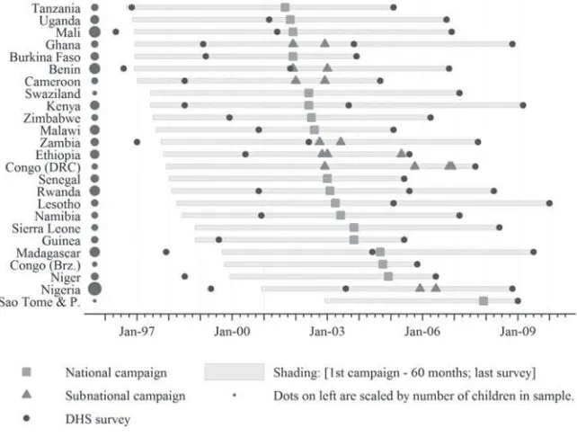
Survey data are merged with the date of the _ﬁ rst national campaign in the respon-dent’s country. In seven countries, campaigns were conducted at different times for different subnational regions; in these instances, we split the country into subnational “campaign- regions.” Figure 1 displays the timing of the catchup campaigns in each country in our sample and the timing of the DHS surveys. We use the term “campaign- region” to denote either the country or subnational region in which a unique campaign occurred. Appendix A includes additional details on the SIAs and surveys.

Our main sample consists of children who were born no more than seven years before the launch of an MI SIA (N = 566,806). Column 2 in Table 1 shows that 68,495 children died before their _ﬁ fth birthday, and the data for 305,513 of the observations are truncated (that is, the child was alive and less than _ﬁ ve years old at the time of the Figure 1

Timeline of Measles Initiative SIAs and DHS surveys

Sources: MI publications, correspondence with MI staff, and tabulations of DHS data.

(7)

522

Table 1

Summary Statistics from DHS Data

Entire Data Seta

Main Sample:

Children Born ≤ 7 Years

Before Campaign Born 1997 to 2001

Countries (N) 25 25 25

Surveys (N) 52 52 49

Households (N) 317,674 262,213 246,677

Children (N) 893,524 566,806 591,929

Alive at date of survey, age ≤60 months 350,896 305,513 145,229

Alive at date of survey, age >60 months 413,576 190,463 351,382

Reported death before 60 months 121,652 68,495 89,138

Reported death at age ≥60 months 7,400 2,335 6,180

Mean hypothetical age at interview (months) 59.9 53.3 89.7

Mean hypothetical age at campaign (months) 75.8 27.0 77.0

Number of child- months in panel data

Birth to interview or 60 months 42,434,559 23,675,263 16,874,094

Birth to death, interview, or 60 months 37,677,665 21,226,237 14,848,412

Mean age in panel data (months) 26.4 24.9 28.4

Source: Authors’ calculations with DHS data.

(8)

523

interview). The seven- year cutoff was chosen so that two years’ worth of data are used to estimate precampaign trends in childhood mortality rates (that is, mortality through ﬁ ve years of life). Because of the variation in the campaign timing, this approach entails samples for each country spanning different time periods.

The primary advantage of the DHS is the standardized, nationally representative birth and death histories provided across samples. There are also several limitations to this data. First, by capturing these histories from each adult woman respondent, the DHS omits maternal orphans. If these orphans experience differential measles- related mortality rates, our estimated treatment effects may not be representative of the en-tire child population. In addition, if maternal orphanhood is also correlated with the speci_ﬁ c timing of the campaigns (conditional on smooth campaign- region- speci_ﬁ c time trends), our estimates may exhibit selection bias. One major source of variation in maternal orphanhood rates may be the changing prevalence of HIV/AIDS across Africa in our time period. To test this, we merge data from the World Development Indicators (WDIs) on the country- level share of the adult population (aged 15–49) infected with HIV with the campaign dates. Changes in this share between 1996 and 2001 (the primary birth years in our sample) exhibit only weak correlation with the campaign dates at the country level (0.05, p- value = 0.81), suggesting that differential maternal mortality rates due to HIV are unlikely to be a major source of bias.

A second limitation is that the DHS does not uniformly ask mothers for the cause of death of any deceased child. Thus, we are limited to assessing all- cause mortality and cannot speci_ﬁ cally examine measles- related deaths. Even if the question had been asked, however, it might not have been reliable because we would expect underreport-ing of measles- related deaths in survey responses in cases where measles is a contrib-uting factor to deaths from diarrhea and other causes (Walker et al. 2013).

The DHS asks each mother about the immunization histories for each living child; children who received the measles vaccine but died of other causes are thus omitted in this data. In addition, when the mother has a yellow vaccination card or other record, the DHS enumerator records these details in the survey. Unfortunately, in our sample fewer than 50 percent of children have vaccination cards that are observed by the DHS enumerator. Where these cards are unavailable, maternal recall of the dates of any vac-cinations is known to be both extremely noisy and biased (see Suarez et al. 1997; Bolton et al. 1998; and Watson et al. 2006 for examples in developed country settings, and Murray et al. 2003 for a developing country study); as a result, household- retained cards and parental recall are often insuf_ﬁ cient sources of information for estimating population coverage rates (for example, Luman et al.2008). Considering both the sample selection in measuring vaccine coverage among surviving children and the biases in estimating vaccination timing, we do not use the DHS data to measure the extent or timing of indi-vidual vaccinations as intermediate outcome variables for the SIAs.4

The DHS asks respondents for the length of time they have lived in their current loca-tion but not for speci_ﬁ c prior locations: We thus merge the MI campaign dates on the

(9)

respondents’ current locations. For countries with subnational campaigns, this may misas-sign dates for respondents who have migrated across the relevant subnational regions. In the results presented below, we conduct two checks to ensure this potential misassign-ment does not bias our results: We omit countries with subnational campaigns, and we omit respondents who have moved to their current location in or after 2001 (the year of the _ﬁ rst campaign).

Age heaping is also an important concern in the DHS data; the age at death is dispro-portionately likely to be reported at 0, 12, 24, 36, 48, and 60 months. Although the DHS interviewers ask about the age at death in months of each child who has died, respondents may “round” this age to 12- month intervals. Unfortunately, the speci_ﬁ c parameters of this rounding are not known (such as direction, symmetry). Although this heaping is unlikely to be correlated with the campaign timing, it does introduce additional measurement error, which could attenuate our results toward zero. To address this concern, we adopt conserva-tive approaches for our baseline estimates and then conduct sensitivity checks by reassign-ing age- at- death usreassign-ing various rules. We discuss these results in the respective sections but, in each case, they remain qualitatively similar to those in our baseline estimates.

IV. Child- Level Analysis

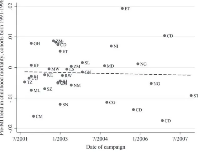
We begin by testing whether campaign timing is correlated with pre-vious trends in childhood mortality rates (that is, whether the pre- MI mortality trends are indeed parallel across treatment status—here, campaign timing indicating treat-ment timing). To do so, we use an alternate sample of older children born between 1991 and 1996 (cohorts who were at least _fi ve years old when the _fi rst campaign took place) and estimate campaign- region speci_fi c trends in their birth years, as follows: (1) Survivalitc =␭c+␥t+␾c*t+εitc,

where Survivalitc is the survival to 60 months of child i born in year t in campaign- region c, ␭_c are campaign- region- speci_fi c dummies, ␥_t are birth- year dummies, and ␾_c*t are linear trends in birth year speci_fi c to each campaign- region. We estimate this speci_fi cation via ordinary least squares and plot the estimates of ␾_c against the timing of the campaigns (Figure 2). We _fi nd no correlation between these estimated trends and campaign timing, suggesting that pre- MI mortality trends are not meaningfully different for those regions with earlier campaigns. Appendix A includes a map of campaign dates timing showing that the earlier campaigns were not focused on a particular region of the African continent.

To estimate our primary treatment effects of interest, we return to our main sample of children born after 1997. We estimate the effects of the SIAs on childhood survival using a logit regression model with child- level data:

(2) Pr(Survival to ␣_itc | Xitc)

= F(Hyp Age At Campaignitc␤+␭c+␥t+␾c*t+ Xitc␯),

where F(u) = exp(u) / (1 – exp(u)). Our dependent variable Survival to ␣_itc is a dummy variable indicating whether the child survived at least _␣months, and we run separate regressions for ␣ equal to 1, 12, 24, 36, 48, and 60 months. (Levels of ␣ were selected

(10)

necessitates that we limit our sample in each regression to children for whom the DHS interview was conducted at least _␣months after their birth. (Sample sizes are thus larger when _␣ is smaller.)

Our treatment measure Hyp Age At Campaign_itc is the time elapsed between the child’s birth and the launch of the MI campaign in the campaign- region.5_We catego-rize this timing into the following groupings, including a dummy variable for each: born after the campaign or 0–11, 12–23, 24–35, 36–47, and 48–59 months prior (with a reference group of children born 60–83 months prior). We include birth- year dum-mies (␥_t) to control for continent- wide variation in annual survival rates (separately by gender), as well as campaign- region- speci_fi c dummies (␭_c) and campaign- speci_fi c birth- year trends (␾_c*t) that control for gradual changes in local survival rates. Other individual controls (X_itc) include the child’s gender and her mother’s edu-cation and age at _fi rst birth. Note that some children died prior to the campaign; for these children, Age At Campaign_itc is the hypothetical age at the campaign had they survived.

5. In our full sample of children, the age at campaign varies between births 84 months prior to a campaign and 56 months after a campaign; when we limit the sample to those whose full childhoods are observed, the youngest child in the sample is born six months after a campaign.

Figure 2

Pre- Measles Initiative trends in mortality and campaign timing

Notes: This ﬁ gure plots the estimate of ␾c from Equation 1 for each country against the date of the MI

(11)

Our model can be interpreted as a difference- in- differences estimator of the cross- cohort, cross- campaign- region differences in survival rates based on exposure to the cam-paigns. Within a given campaign- region, older cohorts that were born more than _fi ve years prior to the campaign serve as comparisons for younger cohorts exposed to the campaigns during their childhoods. At the same time, cohorts in other regions allow us to control for birth- year effects with both birth- year dummies and campaign- region- speci_fi c birth- year trends, as well as for campaign- regionwide effects. Impacts are identi_fi ed by comparing differences between older and younger cohorts in the countries with earlier campaigns to the differences between the older and younger cohorts in countries that have not yet received the campaign (Imbens and Wooldridge 2009, pp. 67–69; Angrist and Krueger 1999, pp. 1296–99). We estimate the above regression using the DHS survey weights and report Huber- White adjusted standard errors, clustered at the campaign- region level (following Bertrand, Du_fl o, and Mullainathan 2004).

Our primary results for survival until 60 months indicate that children born fewer than 36 months prior to an SIA are signi_ﬁ cantly more likely to survive their childhood than are those born 36 or more months prior to the campaign (p- value = 0.002).6_{In Table} 2, we present the speci_ﬁ c results, showing that a child who was born immediately after the campaign was 10.2 percent less likely to have died within 60 months of birth than a child who was born more than 60 months prior to the campaign. These effects decrease monotonically in the time elapsed between birth and the campaign, to the point that chil-dren born 36–60 months prior to the campaign are no more likely than older cohorts to survive until 60 months. The overall treatment effect from this model is estimated at 2.4 percentage points (weighting treatment effects by the age of each child at the campaign).

The results for survival until 48 and 36 months (Columns 2 and 3 of Table 2) are qualitatively similar but monotonically smaller. We see no signi_fi cant differences in survival to younger ages. In particular, we _fi nd no differences in survival to 12 months (Column 5) and one month (Column 6) by age- at- campaign, consistent with the measles vaccination taking place after nine months of age. The absence of signi_fi cant effects on survival to 24 months is notable but likely due to the short exposure time. As the exposure duration lengthens to older ages (36 months and over), we observe signi_fi cant effects of birth 12–23 months prior to the campaign (that is, signi_fi cant for survival to 48 and 60 months, shown in Columns 1 and 2).7

Next, we estimate the effects of survival to 60 months by gender, interacting the age at campaign categories with gender dummies in the pooled sample (Column 7). We _fi nd the effects are somewhat larger for girls than for boys (with effects for the < 0, 12–23, and 24– 35 age categories statistically different at the 5 percent con_fi dence level), suggesting that the MI bene_fi tted girls more, on average, than boys, regardless of the age at vaccination.

To validate our _ﬁ ndings, we conduct a series of falsi_ﬁ cation tests to ensure that other correlates of public health conditions at the country level are not driving our results. We

6. The p- value reported is from a separate regression similar to that of Table 2, Column 1, where in place of the 12- month bins for birth date relative to campaign date, we include only a single dummy variable indicat-ing a child was born less than 36 months prior to the campaign date.

7. We include indicators for hypothetical ages- at- campaign greater than ␣ for completeness and as a

(12)

fi rst examine prenatal and birth outcomes in our sample. Because measles vaccinations under the MI were not administered until nine months of age, prenatal and birth out-comes should largely remain unaffected by the campaigns.8_{We estimate Equation 2 with} two additional dependent variables: (1) whether the mother received any prenatal tetanus shots during each pregnancy, and (2) whether the child’s weight was rated as “smaller than average” or “much smaller than average” at birth. Both variables are available only for each mother’s last three births, slightly limiting our sample. The results for prenatal tetanus shots (displayed in Table 3, Column 1) show nonmonotonic differences in this outcome across age at campaign bins, and the difference between those born fewer than 36 months prior to the campaign and those born 36–59 months prior is not signi_fi cant (p = 0.427) (children in the 48–59 month category exhibit lower prenatal tetanus coverage than the reference group born at least 60 months prior to the campaign, signi_fi cant at the 5 percent con_fi dence level). The results for low birth weight (Table 3, Column 2) show no signi_fi cant differences in the odds ratios of children born closer to an MI campaign. Taken together, these tests indicate that our primary results are indeed measles- speci_fi c and not likely due to correlations in campaign timing with other public health conditions.

It is also possible that pre- MI mortality events were correlated with the timing of the campaigns and that older cohorts born more than _fi ve years prior to the _fi rst MI campaign thus exhibit similar mortality patterns as those exposed to the campaigns. We test for the presence of such correlation by estimating our primary Speci_fi cation 2 for the older sample of children born between 1991 and 1995. We use a hypothetical campaign date that is _fi ve years earlier than the actual date (a linear transform in the hypothetical age- at- campaign variable) to make the interpretation more comparable to our main results. The results, shown in Column 3 of Table 3, again indicate no differ-ence in survival odds among children born close to this false campaign date. Together with Figure 2, these results suggest that our main _fi ndings are not due to correlation between pre- MI mortality changes and the timing of the campaigns.

Finally, we also consider whether differential cross- country mortality changes in the post- MI period may be driving our results. Our main speci_fi cation includes coun-try dummies and trends (and, for subnational campaigns, campaign- region dummies and trends), but it is possible that these do not adequately control for all time- varying features. We therefore take two approaches to address this possibility. First, in the dura-tion model framework described in the next secdura-tion, we consider a variety of time- varying factors, such as health and security conditions at the country- year level.9 Second, we estimate our main speci_fi cation for several single country samples where subnational campaigns took place (recognizing that sample size may limit the precision of our estimates). We show the results estimated for Benin and Zambia in Columns 4 and 5 of Table 3. Both countries have relatively large samples and suf_fi ciently early campaigns such that we can observe _fi ve years of subsequent survival for a large share of these samples (in both cases, however, there are too few children in the sample who were not yet born at the date of the campaign to estimate a coef_fi cient on this category). For both countries, the marginal effects are decreasing in the age at campaign, as in our base

8. It is possible that the campaigns could have affected fertility patterns; if these effects differed across baseline prenatal and birth conditions, we could observe a compositional effect on these outcomes among our subsample who were not yet born at the date of the campaigns.

(13)

528

Table 2

Main Results from Child- Level Model

1

α = 60

2

α = 48

3

α = 36

4

α = 24

5

α = 12

6 α = 1

7

α = 60

Survival to α Months Girls Boys

Panel A: Odds ratios

Unborn at date of campaign 2.736** 2.145*** 1.686** 1.176 1.068 0.963 3.694*** 2.213*

[1.171] [0.585] [0.352] [0.187] [0.137] [0.148] [1.659] [0.928]

Hypothetical age at campaign 0–11 months

1.971** 1.632** 1.401** 1.140 1.084 1.022 2.032** 1.923**

[0.534] [0.337] [0.212] [0.158] [0.114] [0.147] [0.579] [0.529]

1.464* 1.297* 1.212 1.035 1.014 0.958 1.57** 1.376

[0.296] [0.192] [0.145] [0.120] [0.0962] [0.122] [0.330] [0.276]

1.352** 1.273** 1.170* 1.071 1.082 1.017 1.492*** 1.241

[0.189] [0.136] [0.102] [0.0965] [0.0925] [0.115] [0.226] [0.172]

1.064 1.014 0.997 0.940 0.949 0.914 1.11 1.025

[0.092] [0.075] [0.067] [0.0717] [0.0640] [0.0777] [0.100] [0.092]

0.979 0.951 0.967 0.939* 0.951 0.917 1.014 0.948

(14)

529

Panel B: Implied treatment effect (percentage points)

Unborn at date of campaign 10.2 9.66 5.72 1.38 0.429 –0.117 11.43 8.99

9.22 5.93 3.56 1.14 0.545 — 9.41 9.11

5.21 3.29 2.19 0.329 — — 5.96 4.52

3.66 2.91 1.75 — — — 4.66 2.73

0.84 0.18 — — — — 1.35 0.342

–0.29 — — — — — 0.18 –0.74

Overall 2.37 2.51 2.04 0.471 0.208 –0.131 2.38

Observations 214,815 271,111 333,638 397,885 466,071 538,172 214,815

Mean of dependent variable 85 percent 86 percent 87 percent 89 percent 92 percent 96 percent 85 percent

Pseudo R2 _0.03 _0.03 _0.03 _0.02 _0.02 _0.01 _0.03

Notes: Odds ratios (Panel A) and implied treatment effect (Panel B). The treatment effect is presented as the percentage point change in the survival rate. DHS data are limited to children whose interview date is at least a months after birth and who were born a maximum of seven years before campaign. All models control for gender, mother’s age at ﬁ rst birth, and mother’s education in addition to year of birth dummies, campaign- region dummies, and campaign- region- speciﬁ c time trends. Models use survey weights from DHS. Robust standard errors of the odds ratios, clustered by campaign- region, are in brackets (calculated using the delta rule in Stata 12.0).

(15)

The Journal of Human Resources

530

Table 3

Validation Tests for Child- Level Model

1 2 3 4 5

Dependent Variable Any Prenatal

Tetanus Shots

Smaller than Average Birthweight

Survival to 60 Months (False Campaign Date)

Survival to 60 Months

Sample Baseline Baseline Born 1991–95 Only Benin Only Zambia

Panel A: Odds ratios

Unborn at date of campaign 1.012 0.858 — — —

[0.235] [0.121]

0.845 0.830 1.014 1.091 2.172***

[0.172] [0.115] [0.122] [0.0764] [0.521]

0.783 0.815 0.985 1.172 1.091

[0.123] [0.112] [0.0946] [0.246] [0.0876]

0.804 0.805 0.999 1.031** 0.962

[0.0964] [0.0907] [0.0675] [0.0148] [0.0485]

0.826 0.876 0.972 0.914*** 0.853***

[0.0976] [0.0688] [0.0435] [0.0256] [0.00272]

0.848* 0.952 0.980 0.896** 0.888***

(16)

BenY

ishay and Kranker

531

Panel B: Implied treatment effect (percentage points)

Unborn at date of campaign 0.208 –2.28 — — —

–2.90 –2.76 0.33 1.06 7.11

–4.71 –3.24 –0.36 1.88 1.02

–4.12 –3.34 –0.03 0.377 –0.476

–3.63 –2.01 –0.67 –1.17 –2.04

–3.04 –0.744 –0.49 –1.43 –1.50

Overall –2.46 –2.56 –0.42 –0.105 –0.350

Observations 114,995 184,446 257,543 18,127 7,510

Mean of dependent variable 68 percent 18 percent 83 percent 85 percent 86 percent

(17)

model, but the differences between birth within three years of a campaign and birth more than three years prior are not statistically signi_ﬁ cant in these much smaller samples.

We also conduct a number of robustness checks to assess whether our results are driven by unobserved subnational factors or seasonality, as well as sample selection issues. Table 4 displays the results of these checks. In Column 1, we add dummies for all subnational regions to control for unobserved differences between these areas that may be correlated with differential within- country measles mortality trends. Because measles exhibits regular seasonality patterns that may be correlated with the within- year timing of measles cam-paigns, we further control for seasonality by including month- of- birth dummies (Column 2). Attempts to control for unobserved factors are certain to be imperfect. To better un-derstand the role played by our controls (including campaign- region dummies and trends and individual- level variables), we drop all covariates from our model (estimating only the effects of hypothetical age- at- campaign on survival). The results, shown in Column 3, are quite similar to our baseline _ﬁ ndings (albeit with a smaller overall impact estimate).

In addition, a number of countries in southern Africa had their _ﬁ rst SIAs in the late 1990s (precursors to the MI) so the effects of MI SIAs in these countries may be somewhat muted. In Column 4, we exclude four southern African countries that may have had pre- MI SIAs in the late 1990s (Lesotho, Malawi, Zambia, and Zimbabwe). Next, we consider a bal-anced sample, as our baseline sample inclusion strategy is based on a seven- year window prior to a given campaign, making our baseline sample unbalanced across countries over time. To address this imbalance, in Column 5, we limit our sample to children born in 1997 through 2003. Finally, we consider whether selective migration in anticipation of or in re-sponse to the campaigns may be driving our results. To do so, we limit our sample to only countries with national campaigns where internal migration would not lead us to misassign treatment status (Column 6). In addition, in Column 7, we limit our sample to children whose mothers have been resident in their present location since 2001 (the year of the _ﬁ rst campaign). In all of these instances, the results are similar to those in our baseline model.

Concerning heaping in the age- at- death variables, our main results are for survival to the dates with the most data heaping. That is, our dependent variables in the regression analysis are the months in which the heaping occurs. We use the age- at- death vari-able provided in the DHS survey (b6). We also conduct sensitivity checks reassigning age at death by drawing the age in months from a uniform distribution of ages in the interval [a, a + 11], where a is age- at- death in years, using various reassignment rules: (1) reassign where this variable is reported in the DHS to be imputed, (2) assuming that a share of ages- at- death that are reported to be exactly an integer year (that is, 12, 24, 36, 48 months, etc.) are misreported (we vary this share over 10 percent, 20 percent, and 40 percent of the deaths in the heaped categories). The results (omitted for brevity) are largely unchanged and are quite stable across varying levels of reassignment.

V. Duration Analysis

(18)

regression model to estimate the change in the hazard rate—the probability of death in period t conditional on survival until period t – 1 and covariates—that occurs after an SIA has taken place. The hazard rate is modeled with the following logit probability model:

(3)

Pr( yit =1|yi,t−1≠1, Postct, Xi, Wct)

= F(Postct␦+␮ag + Xi␤+␥m+␩b+␪rq+␭c+␳c*t+Wct␾)

where y_it = 1 if a child (i) died in month t, conditional on survival until age t – 1, and F(u) = exp(u) / (1 – exp(u)). The parameter estimates are interpreted as proportional shifts in the baseline monthly hazard rate. In particular, the variable Postct is a dummy indicating whether an SIA has taken place in the child’s campaign- region (c)in the time period (t) or earlier, and the estimated coef_fi cient _␦ models the average effect of the MI on the monthly child mortality rate. The coef_fi cient ␮_ag captures the mean mortality risk for children with the same age (a) and gender (g), and the vector of control vari-ables X_i includes child- speci_fi c non- time- varying characteristics (gender, mother’s age at _fi rst birth, and mother’s education).

Control variables are used to purge the model of omitted campaign- region charac-teristics and trend effects, time- speci_fi c Africa- wide shocks, and regional seasonality in key variables. To control for seasonality in both birth rates and region- speci_fi c mortality risks that may be confounded with the timing of the SIAs, we include dum-mies for month in time (␥_m), month of birth (␩_b), and Africa region by quarter time dummies (␪_rq, for being born in the third quarter of 2005 in West Africa, for example). The last two terms, ␭_c+␳_c*t, capture campaign- region- speci_fi c means and trends. In alternate speci_fi cations, we interact Post_ct with an array of age group dummies (< 1 month, 1–11 months, 12–23, 24–35, 36–47, 48–59, and 60+ months) to estimate the effect of the campaign by age, or we interact Post_ct with an array of age group dum-mies and gender to estimate the effect of the campaign in each gender- age cell.

As discussed above, we also control for country- level factors that may be related to the timing of MI SIAs across countries (W_ct), potentially confounding our impact estimates. We incorporate time- varying data from the World Bank’s WDIs on con_ﬂ ict (total number of refugees _ﬂ owing from the country), military expenditures (as share of GDP), and health system capacity (DPT immunization rate, TB- detection rate, ag-gregate health expenditures as a share of GDP). When including these covariates, we lose country- year cells for which these WDI variables are unavailable.

We estimate the mean marginal effect implied by _␦, averaging across the treated child- month observations (including “hypothetical” observations up to the 60th month of life or the DHS interview date, whichever occurred _ﬁ rst, regardless of whether the child died). Standard errors, clustered by country, are calculated with the delta method.

A major concern is that our duration models are underpowered, primarily because monthly age- speci_ﬁ c mortality rates are considerably noisier than cumulative childhood survival rates and because we estimate a more sophisticated model. Perhaps counterintuitively, the switch from the child- level data set to the considerably larger child month- level data set does not increase the statistical power because we account for within- group intraclass error correla-tions when calculating standard errors. Although the duration model has less power, it is used to assess the robustness of our child- level results with time- and age- varying covariates.

(19)

534

Unborn at date of campaign 2.857** 3.405*** 2.375*** 2.566** 2.809** 3.068** 3.103**

[1.201] [1.573] [0.320] [1.171] [1.142] [1.606] [1.375]

2.037*** 2.367*** 1.295** 1.730** 2.007*** 1.946* 2.176**

[0.533] [0.683] [0.146] [0.459] [0.520] [0.670] [0.692]

1.493** 1.639** 1.079 1.313 1.482** 1.490 1.623**

[0.289] [0.330] [0.160] [0.268] [0.281] [0.398] [0.382]

1.374** 1.434** 1.266*** 1.283* 1.369** 1.406* 1.402**

[0.182] [0.206] [0.098] [0.176] [0.171] [0.266] [0.218]

1.066 1.089 0.977 1.028 1.076 1.090 1.103

[0.090] [0.096] [0.0536] [0.086] [0.073] [0.126] [0.103]

0.979 0.976 0.932 0.956 0.992 0.965 0.987

(20)

535 Panel B: Implied treatment effect (percentage points)

Unborn at date of campaign 10.6 13.3 8.42 8.7 10.3 11.5 12.1

9.7 12.3 3.13 7.3 9.6 9.3 10.9

5.5 6.9 0.99 3.7 5.4 5.6 6.7

3.8 4.5 2.87 3.0 3.8 4.0 4.1

0.9 1.1 –0.32 0.3 1.0 1.1 1.3

–0.3 –0.3 –0.95 –0.6 –0.1 –0.5 –0.2

Overall 2.5 3.1 0.69 1.6 2.5 2.7 2.7

Observations 214,815 214,776 214,815 187,743 203,410 138,674 169,986

Mean of dependent variable 85 percent 85 percent 85 percent 85 percent 85 percent 85 percent 85 percent

Pseudo R2 _0.04 _0.03 _0.03 _0.03 _0.03 _0.03 _0.02

Notes: Odds ratios (Panel A) and implied treatment effect (Panel B) for child survival to age 60 months. The treatment effect is presented as the percentage point change in the survival rate. DHS data are limited to children where interview date is at least 60 months after birth and who were born a maximum of seven years before campaign. All models control for gender, mother’s age at ﬁ rst birth, and mother’s education in addition to year of birth dummies, campaign- region dummies, and campaign- region- speciﬁ c time trends. Models use survey weights from DHS. Robust standard errors of the odds ratios, clustered by campaign- region, are in brackets.

(21)

536

Table 5

Implied Mean Marginal Effects from Duration Model

Death in Month t

for Child i (Treatment

Effect, Percentage Points)

1 2 3 4 5 6 7

Base

Interact with Age

and Gender Break

in Time Trends

Security Controls

Health Sector Controls

Security and Health

Controls

Boys Girls

0 to 60 months old –0.0135

[0.0103]

< 1 month old –0.0234 –0.0404 –0.00608 –0.0417 –0.114 –0. 0756 –0.0547

[0.161] [0.224] [0.122] [0.2046] [0.164] [0.148] [0.156]

1–11 months old –0.01475 –0.0157 –0.0138 –0.0174 0.00633 0.00773 0.0132

[0.01679] [0.0201] [0.0158] [0.0211] [0.0209] [0.0194] [0.0209]

12–23 months old –0.0315** –0.0369** –0.0260 –0.0329** –0.0358*** –0.0320*** –0.0319***

[0.01365] [0.0135] [0.0154] [0.015] [0.0102] [0.00993] [0.0107]

24–35 months old –0.00489 0.000418 –0.0103 –0.0058 –0.000343 0.00606 0.00599

[0.0096] [0.0122] [0.00970] [0.0106] [0.00912] [0.00938] [0.0101]

36–47 months old –0.00388 –0.000887 –0.0693 –0.0048 –0.00219 0.00191 0.00144

[0.00643] [0.00707] [0.00751] [0.007] [0.00665] [0.00642] [0.00724]

48–59 months old –0.00326 –0.00245 –0.00409 –0.0044 –0.00220 –0.000471 –0.000334

[0.0039] [0.00527] [0.00455] [0.0043] [0.00348] [0.00401] [0.00396]

60 months old 0.00269 0.00269 –0.00166 0.0003 –0.00119 –0.00146 –0.00156

(22)

537

Gender by age dummies Yes Yes Yes Yes Yes Yes Yes

Country by campaign- region dummies

Yes Yes Yes Yes Yes Yes Yes

Country by region trends

Month time dummies Yes Yes Yes Yes Yes Yes Yes

Month of birth dummies Yes Yes Yes Yes Yes Yes Yes

Africa region by quarter dummies

Post_t interacted with

campaign- region time trend

Yes

Military controlsa _Yes _Yes

Health sector controlsa _Yes _Yes

Observations (child- months)

21,226,237 21,226,237 10,700,116 +10,526,121 21,226,237 18,382,849 18,271,038 17,486,535

Survey weights Yes Yes Yes Yes Yes Yes Yes

Weighted population size 14,300,343 14,300,343 14,300,343 14,300,343 11,988,362 11,988,362 11,910,017

Notes: Implied mean marginal effects from logit regression, where dependent variable is a dummy for a child’s death in month t, using children who lived through month t–1. The treatment effect is presented as the percentage point change in one- month mortality rate. Robust standard errors, clustered by campaign- region, are in brackets. Models use survey weights from DHS.

*** p < 0.01, ** p < 0.05, * p < 0.1

a _{Time- varying control variables from the World Bank’s WDIs on con}

(23)

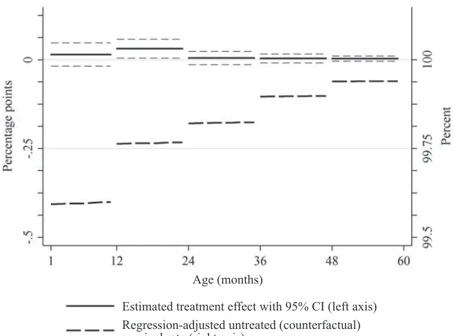
effects are estimated separately for each age group (using interaction terms), our point estimates indicate that reductions in child mortality are concentrated in children’s _fi rst 24 months of life (p = 0.03), while mortality reductions are an order of magnitude smaller at older ages (Column 2). Figure 3 plots the impact estimates by age group, revealing the inverted- U pattern. The MI appears to have larger effects on the _fi rst 24 months of life because those are the ages where baseline survival rates are lower. (For comparison, Figure 3 also includes the counterfactual survival rates on the same scale.) These are also the ages where measles- speci_fi c CFRs are the highest (Stein et al. 2003; Wolfson et al. 2009). At older ages, comparison group survival rates are higher, leaving less “room” for large- magnitude treatment effects, and a larger number of older children might have gained immunity through prior infection and thus would not bene_fi t from vaccination.

We extend the model further by interacting the age- speci_ﬁ c estimates with a gender dummy in the pooled sample (Column 3). We _ﬁ nd marginal effects of the campaigns

Age (months)

Estimated treatment effect with 95% CI (left axis) Regression-adjusted untreated (counterfactual) survival rate (right axis)

Figure 3

Effect of MI on monthly survival rates from 1 through 60 months from duration model Notes: The solid line plots the effect of the MI on monthly survival rates (left axis) from the model in Table 5, Column 2. The estimates for the fi rst month of life are omitted because the confi dence intervals are of a different order of magnitude. The thick dashed line plots the counterfactual survival rate (right axis), which is defi ned as the mean of the predicted values obtained from the regression model under the counterfactual scenario of no MI campaign, where the predicted values are averaged across the children who were in fact treated by the MI campaigns. This regression adjustment smooths out age heaping and statistical noise and adjusts for any differences between the treatment and comparison groups in the control variable distributions. The two axes are on the same scale: The vertical distance between the horizontal lines is 25 basis points on both axes.

(24)

are larger for boys than girls in the second year of life, but these effects are not statis-tically different. In the fourth model presented in Table 5, we introduce an additional term into Equation 3: Post

ct* (␳c*t). This speciﬁ cation allows overall mortality levels and trends to differ between treatment and comparison groups in the preperiod and allows the levels and trends within a campaign- region to differ before and after the campaign. Because our models identify the differential effects of the campaign across ages, our estimation is robust to this additional term. This approach further allows us to control for any local discontinuities in mortality rates around the campaign date. The results, reported in Column 4 of Table 5, show that campaign effects are statisti-cally signi_ﬁ cant in the second year of life.

In the duration model framework, one can easily and intuitively control for time- varying factors that may have also been correlated with campaign timing and mortality changes. In the remaining columns in Table 5, we incorporate time- varying (country- year level) refugee, military, and health system capacity variables from the WDI. These variables have relationships to mortality rates consistent with intuition: Mortal-ity rates are higher in years when refugee out_ﬂ ows are larger (p = 0.02), when military expenditures are larger (p = 0.30), and when health expenditures are lower (p = 0.06). Nonetheless, the primary effect of interest—that of the MI SIAs—remains unchanged, suggesting that correlation between SIA timing and broader changes in mortality risks does not drive our results.

As in the case of the child- level model, we conducted a number of robustness tests to verify that the results were unchanged if we used alternative sample de_fi nitions. First, we reestimate the duration model with various sample de_fi nitions (Table 6): (1) children born between 1997 and 2001; (2) all child- month observations in our data set; (3) children born between 1997 and 2003; (4) children born fewer than _fi ve years prior to each campaign; (5) dropping Lesotho, Malawi, Zambia, and Zimbabwe (the countries with pre- MI SIAs); (6) including only those countries with pre- MI SIAs;10 and (7) dropping Nigeria, which accounts for a disproportionate share of our sample. Our results remain quite similar across all of these tests. For example, the treatment effect point estimate for observations between the age of 12 months and 23 months varies by only a few basis points (2.5 to 5.2).

To address age heaping, our main results are based on death variables that, for chil-dren who die when aged over two years, use the midpoint between the two birthdays (for example, a response of “two years” is interpreted as two years, six months), adjust-ing for cases in which the child died in the year of the interview. This approach follows that of Rajaratnam et al. (2010).If respondents primarily round down, this approach will be conservative because children are more likely to die at younger ages, and we therefore would shift too many deaths from the baseline to intervention periods. That is, this adjustment shifts some deaths that actually occurred in the “pre” period and treats the deaths as if they occurred in the “post” period, thereby attenuating im-pact estimates toward zero. We also assess whether our main _ﬁ ndings are robust to

(25)

540

Table 6

Duration Robustness Checks

1 2 3 4 5 6 7 8

Death in Month t for

Child i (Treatment Effect,

Percentage Points)

< 1 month old –1.30*** –0.288 –0.213 0.172 –0.0455 0.157 –0.106 –0.0234

[0.361] [0.195] [0.235] [0.159] [0.177] [0.248] [0.164] [0.161]

1–11 months old –0.0267 –0.0453** –0.0134 0.00505 –0.0127 –0.0389 –0.0213 –0.0147

[0.0527] [0.0182] [0.0266] [0.0164] [0.0176] [0.0369] [0.0191] [0.0168]

12–23 months old 0.00378 –0.0436*** –0.0427*** –0.0250** –0.0282* –0.0522* –0.0433*** –0.0315**

[0.0216] [0.0136] [0.0117] [0.0120] [0.0151] [0.0171] [0.00920] [0.0136]

24–35 months old –0.0278 –0.0156* –0.00634 0.00781 –0.00336 –0.0144 –0.00983 –0.00489

[0.0678] [0.00810] [0.0124] [0.0103] [0.0107] [0.0138] [0.00968] [0.00960]

36–47 months old –0.0162 –0.0145** –0.00140 –0.00377 –0.00125 –0.0238 –0.00877 –0.00388

[0.0443] [0.00617] [0.00663] [0.00852] [0.00680] [0.0142] [0.00522] [0.00643]

48–59 months old –0.0135 –0.00682 –0.00198 –0.0000578 –0.00245 –0.00915 –0.00551 –0.00326

[0.0176] [0.00402] [0.00330] [0.00763] [0.00424] [0.00608] [0.00370] [0.00390]

60 months old — 0.00619 –0.000985 — 0.000744 — 0.000141 0.000535

(26)

541

Gender by age dummies Yes Yes Yes Yes Yes Yes Yes Yes

Country by region dummies

Yes Yes Yes Yes Yes Yes Yes Yes

Country by region speciﬁ c time trends

Month of birth dummies Yes Yes Yes Yes Yes Yes Yes Yes

Month of birth dummies (1,2,3, . . . 12)

Africa region by quarter time dummies

Children 554,889 893,524 394,551 430,211 485,455 81,351 507,436 566,806

Number of observations (child- months)

14,847,572 37,677,665 16,523,653 14,890,995 18,269,973 2,931,330 19,003,352 21,226,237

Weighted number of observations

7,784,786 21,942,953 10,806,650 10,976,435 1,251,9213 1,768,525 12,845,782 14,300,343

Notes: Implied mean marginal effects from logit regression, where dependent variable is a dummy for a child’s death in month t, using children who lived through month t–1. The treatment effect is presented as the percentage point change in one- month mortality rate. Robust standard errors, clustered by campaign- region, are in brackets. Models use survey weights from DHS. *** p < 0.01, ** p < 0.05, * p < 0.1

(27)

smoothing age at death using a uniform distribution (drawing an age from the interval between the two birthdays). The results are shown in Column 8 of Table 6. We also con_fi rm robustness using the raw data (not reported). Throughout, we _fi nd that age heaping corrections do not affect our primary _fi ndings.

Finally, we also verify that our results are unchanged if we control for mean mor-tality risk and trends in this risk at the subnational rather than national level or if we include a fourth- order polynomial in time to account for any nonlinearities in our primary time trends that may be correlated with SIA timing (results omitted for brevity).

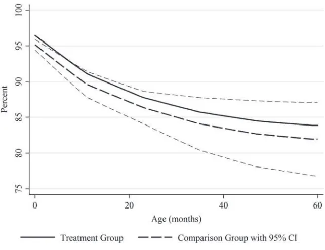
To compare our duration model results with our child- level results and other stud-ies, we calculate the corresponding cumulative reduction in mortality risk over the 60 months of childhood. To do so, we calculate the predicted values from the logit model, Prn( y_it =1|Post_ct). We then take the average of this predicted value across the observations in the sample that had Post_ct = 1 to calculate the monthly mortality rate for the treated observations. We then calculate the counterfactual monthly mortality rate for the same observations, Prn(y_it =1|Post_ct =0, ). We then use a life- table ap-proach to calculate the resulting survival probabilities to obtain a cumulative survival through 60 months under the actual and counterfactual scenarios. These cumulative survival rates are plotted in Figure 4. (Standard errors and con_fi dence intervals were obtained using the delta method.) The difference in the cumulative survival rates is 1.9 percentage points at 60 months, although this effect is imprecisely estimated (95 percent CI –3.0 to 6.9).11_{The point estimate, however, is similar to (but smaller} than) the result from our child- level model (2.4 percentage points), suggesting that our child- level _fi ndings are not unduly in_fl uenced by omitted time- and age- varying controls.

The child- level and duration model both show quantitatively larger effects of vac-cination at younger ages. The child- level model indicates that survival to two years of age (or longer) is linearly decreasing in the child’s hypothetical age- at- campaign (although these effects do not become statistically signi_ﬁ cant until one examines sur-vival to three years). The duration model, meanwhile, suggests that the arrival of a campaign prior to a child’s second birthday (particularly during her second year of life) is most likely to raise her survival probability. The differences may be due to the conditional nature of the duration model, which examines mortality risks at each age given survival to the prior age. This both adjusts the results for differences in baseline survival ages to each age (which the child- level model does not) and also estimates the effects of the campaigns within each interval (and not beyond it).

The models also vary in their gender- speci_ﬁ c estimates, with larger effects esti-mated for girls in the child- level model, while the reverse is largely true in the du-ration model. These model differences again may be due to differences in baseline survival rates to each given age for boys and girls, as well as differences in the timing of the impacts across intervals.

(28)

VI. Discussion

Our survey- based mortality estimates can be compared with the based _fi ndings from Wolfson et al. (2007), which studies measles mortality reductions in sub- Saharan Africa over the same time period. This study’s results imply a 1.47 percent-age point decline in mortality rates across Africa between 2000 and 2005 (see Appendix B). We estimate that 95.1 percent of children in sub- Saharan Africa lived in a country with an MI catchup campaign between 2000 and 2006 (all except Sudan, São Tomé and Principe, Seychelles, and part of Equatorial Guinea), so our model suggests that the MI accounts for a (2.37 * 0.951 =) 2.25 percentage point reduction in child mortality across all children (or 1.91 * 0.951 = 1.81 based on our duration results). Wolfson et al.’s (2007) estimate is somewhat smaller than our point estimates from both the child- level and du-ration analysis but falls within our 95 percent con_fi dence intervals. Simons et al.’s (2012) estimates for 2012 are also smaller than our point estimates, but the time periods are different. These models’ estimates also do not account for underattribution of measles as a cause of death, particularly when diarrhea is cited as the _fi nal cause of death but Figure 4

(29)

measles serves as a contributing factor. Walker et al. (2013) _ﬁ nds that, in some contexts, the effect of measles vaccinations on all- cause mortality can be twice as large as that on measles- speci_ﬁ c deaths. Our estimates account for such indirect effects from measles vaccination, which may be one reason they are larger than those found previously.

The MI vaccination process in the _fi rst decade of SIAs was relatively inexpensive, typically costing slightly less than US$1 per child vaccinated (Christie and Gay 2011). The catchup campaigns vaccinated children up to 15 years of age to eliminate the transmission of measles through older cohorts. Thus, children under age _fi ve represent 38.3 percent of all children vaccinated. Given this cost level and assuming no mortal-ity impacts on children aged _fi ve to 15 years, we calculate a back- of- the- envelope cost- effectiveness measure of $109 per child life saved for our child- level model.12 This _fi gure is remarkably low by international standards. For example, Bryce et al. (2005) calculates that 23 interventions aimed at eliminating 90 percent of global child-hood deaths had an average cost per child life saved of $887.

This estimate of cost- effectiveness is quite low partly because it is based on all- cause rather than measles- speci_fi c mortality. Although we do not directly test for the presence of complementary risks, our results are consistent with complementary risks that are larger than competing risks (that is, reductions in measles cases are likely to reduce mortality risks from other causes rather than increase these risks). Policy-makers should thus consider the health bene_fi ts of measles vaccination more broadly than measles- speci_fi c morbidity and mortality reductions.

Because data are limited, and the difference in the timing of the campaigns across our sample spans only slightly more than four years, we cannot identify the longer- term impacts of the catchup campaigns. Subsequent campaigns aimed at main-taining high coverage rates—recommended at three- to four- year intervals (see Otten et al. 2005)—are dif_ﬁ cult to capture separately in such a framework because the onset of followup SIAs is likely to be correlated with the timing of the initial SIAs.

VII. Conclusions

We assess the impacts of the MI catchup campaigns on all- cause child mortality rates using an identi_ﬁ cation strategy that controls for contemporaneous trends and other potential biases. Using both child- level and duration analyses, we obtain results consistent with a two to three percentage point decrease in this mortality rate due to the campaigns—a notable reduction that is equivalent to 15–19 percent of the baseline childhood mortality rates in our sample (15 percent).

Our study demonstrates the feasibility of using an evaluation approach that relies on variation in the timing of campaigns across countries from exogenous factors (un-related to the outcomes of interest). Our approach offers several advantages over the traditional model- based methodologies because program effects are directly (empiri-cally) measured. This framework may be useful for estimating the effect of the MI on other outcomes and for estimating the effect of other programs (principally those