Consumption Data?
Erich Battistin
Raffaele Miniaci
Guglielmo Weber
a b s t r a c t
In this paper, we use two complementary Italian data sources (the 1995 ISTAT and Bank of Italy household surveys) to generate household-specific nondurable expenditure in the Bank of Italy sample that contains relatively high-quality income data. We show that food expenditure data are of comparable quality and informational content across the two sur-veys, once we properly account for heaping, rounding, and time averag-ing. We therefore depart from standard practice and rely on the estima-tion of an inverse Engel curve on ISTAT data to impute nondurable expenditure to Bank of Italy observations, and show how we can use these estimates to analyze consumption age profiles conditional on demo-graphics. Our key result is that predictions based on a standard set of de-mographic and socioeconomic indicators are quite different from predic-tions that also condition on simulated food consumption, in the sense that their age profile is less in line with the implications of the standard con-sumer intertemporal optimization problem.
Erich Battistin is a research economist at the Institute for Fiscal Studies, London. Raffaele Miniaci is a professor of economics, Padua University. Guglielmo Weber is a professor of economics, Padua Uni-versity, IFS and CEPR. The authors are grateful for helpful discussions with Enrico Rettore, Jean-Marc Robin, Nicoletta Rosati, and Nicola Torelli and for comments by two anonymous referees and au-diences at ESEM99, UCL, UCY, Universita` di Padova, INSEE, Banca d’Italia, the ESRC Econometric Study Group Conference (Bristol 2000), TMR Pensions and Saving Meeting (Paris, 2000) and the ISR-International Panel Data Conference (Ann Arbor 2000). They would like to thank Viviana Egidi and Giuliana Coccia from Istat, and Giovanni D’Alessio from the Bank of Italy for making the data avail-able. This research was financed by CNR and MURST and sponsored by the ISTAT work group explor-ing the feasibility of constructexplor-ing an integrated data bank on household consumption and income from ISTAT and Bank of Italy survey information. To contact the authors, email erich_b@ifs.org.uk [Submitted June 2001; accepted August 2002]
ISSN 022-166X2003 by the Board of Regents of the University of Wisconsin System
Consumption is a key quantity in economics: Standard models as-sume that households derive utility from their consumption of goods and services. In the simplest case, consumption coincides with expenditure (this is normally as-sumed to be true for the purchase of nondurable goods and services) and this moti-vates economists’ interest in using survey data that contain records of expenditure by individual households. In many countries, such expenditure data are regularly collected by asking households to fill out diaries covering all purchases made within a short period. There is a consensus that this time-consuming task produces the best quality expenditure data for small items, while recall questions should also be asked on the purchase of bulky, durable items.
The key problem with diary surveys is that the questionnaire normally focuses on consumption alone, given time constraints and survey practice. A good example is the U.S. Consumer Expenditure Survey (CEX): This uses two representative sam-ples of the U.S. household population. One sample is asked to fill out a detailed expenditure diary over a two-week period and to answer a few questions on house-hold structure (plus a single recall question on food consumption). Another sample is subject to a thorough interview on all aspects of their behavior (including work activities, ownership of major durable goods, income and wealth) that covers broad consumption groups (such as food). The former sample is only contacted once, whereas the latter is asked to participate four more times. In some countries (most notably the United Kingdom), respondents are successfully asked detailed questions on work activities and income before filling out an expenditure diary but no attempt is made to contact them again.
The ideal data set for economists is a panel containing information on a number of aspects of consumer behavior (consumption, leisure and work, wealth, etc.) that covers a long period. Given that ideal, and that keeping diary records is highly time-consuming, the issue then arises of whether consumption information based on recall questions is of comparable quality to information based on diary records.
An extreme, interesting example of recall consumption questions is contained in a widely used Italian survey, the Bank of Italy Survey on Household Income and Wealth (SHIW). It asks respondents a very broad range of questions includ-ing one on their average monthly expenditure on all items and on a few listed durable goods and another on monthly expenditure on food alone. It is worth noting that SHIW contains a large panel component, even though we do not use this feature here.
This paper aims to investigate the quality of consumption data in SHIW to derive measures of the nondurable expenditure alternative to the observed one. We compare the consumption information in SHIW to the corresponding information in a newly released diary-based survey run by the Italian Institute for Statistics (ISTAT), the Survey on Family Budgets (SFB). We concentrate on a single year, 1995, because for that year we gained access to the most disaggregate version of the SFB and were able to construct expenditure items in SFB that are fully comparable to the Bank of Italy definition used in SHIW.
How-ever, we also show that food expenditure data are of comparable quality and informa-tional content across the two surveys, once we properly account for heaping, rounding, and time averaging, whereas for other expenditure definitions (nondurable and total) there are major differences across the two surveys.
This prompts us to compare three different methods to improve the observed mea-sure of nondurable consumption in SHIW: A straight correction for heaping and rounding that makes no use of SFB information; a standard regression-based match-ing method that exploits common information on household characteristics; and a more innovative matching algorithm that exploits common information on household characteristics as well as simulated food expenditure information to predict total nondurable expenditure in the SHIW sample.
We show the implications of these alternative procedures for consumption and saving age profiles in SHIW. It is in fact quite puzzling for an economist to observe that Italian households appear to be saving an increasingly larger proportion of their disposable income as they age. This is apparently due to a marked decline in reported consumption of nondurable goods and services. Given that SHIW is known to have better income and wealth data than SFB, we try to assess whether SFB-based mea-sures of consumption can help solve this puzzle.
The paper is organized as follows. Section II provides some evidence on the pres-ence of measurement error affecting retrospectively asked questions about consump-tion. Section III describes the two data sources and compares descriptive statistics and histograms after we make allowances for sampling differences. Section IV pro-poses a theoretical framework for the matching exercise that takes into explicit ac-count the heaping and rounding problem. Section V describes the method used to correct for heaping and rounding in our application and presents estimation results for the conditional heaping process. Section VI presents regression estimates for nondurable consumption in SFB. Section VII reports estimation and prediction re-sults of the heaping correction for both food and total nondurable consumption. Sec-tion VIII discusses the implicaSec-tions of the imputaSec-tion exercise for nondurable con-sumption in the SHIW sample, with special reference to the resulting age profiles of consumption and the saving rate. Section IX concludes.
II. The Nature and Consequences of Recall Errors
data contain more reliable information about durables and income than about residual items like food and nondurables. In fact, the key reason to doubt SHIW nondurable information about consumption data is the difficulty of the question, in which house-holds are retrospectively asked for their average monthly expenditure over the previ-ous year. The exact wording is: ‘‘What was your family’s average monthly expendi-ture in 1995 for all consumption items? Consider all expenses, including food, but excluding those for: housing maintenance; mortgage instalments; purchases of valu-ables, automobiles, home durables and furniture; housing rent; insurance premi-ums.’’ This question is then followed by a similar food question: ‘‘What was your family’s average monthly expenditure for food alone? Consider expenses on all food items in grocery stores or similar food stores and expenses on meals normally con-sumed out.’’ It included detailed questions on other items excluded from nondurable consumption.
On the other hand, there is also evidence on unreasonably high saving rates com-puted based on SHIW data. The standard aggregate measure defined as (1—total expenditure/disposable income) is 23.4 percent, versus the National Accounts (NIPA) equivalent of 18.2 percent in 1995 (see Banca d’Italia 1999). This discrep-ancy is not particularly large, but becomes worrying if we consider that SHIW in-come falls some 34.7 percent below what the NIPA would imply (see Brandolini 1999, for further details).
Age profiles strongly contradict what one might expect from theory and (to a lesser extent) evidence for other countries. As shown in Brugiavini and Padula (2001), in the cross-section mean individual saving rates increase from 10 percent to 25 percent between the ages of 25 and 60, and then stay above 20 percent for all ages above 60. A slight decline after age 70 is instead observed for median saving rates, but the typical median rate still exceeds 20 percent. Even if we account for a fall in the degree of consumption smoothing around the time of retirement (as pointed out by Banks, Blundell, and Tanner 1998), it is hard to understand why so much saving should take place in old age.
Retrospectively collected information of household surveys are typically charac-terized by recall errors. In particular, respondents are likely to round off the true measure causing abnormal concentrations of values in the empirical distribution. For instance, when we plot histograms of food expenditure on the various waves of the U.S. CEX Diary sample, we see marked peaks at round values, particularly at $50 and $100. Similar evidence can be produced using panel data sets, such as the U.S. PSID and the U.K. BHPS, where a recall question on average monthly expenditure of food is routinely asked.1
As we will show in the next section, the same kind of error clearly affects con-sumption-related variables in the SHIW sample. Such rounding and heaping process makes the relationship between what we aim to measure and what we actually ob-serve complicated compared to classical additive error structure assumptions. The
sign of the bias induced by nonclassical measurement error cannot easily be assessed without imposing distributional assumptions on the process leading to the error-affected measure.
Validation data, that is, observations on the variables of interest collected from an independent assessment of validity study, are useful—when available—to infer on the error structure of observed variables. Bound, Brown, and Mathiowetz (2001) review the state of the art about measurement error results from validation studies across a wide range of areas in economics.
Along the same lines, in what follows we aim to shed more light on the quality of information about consumption contained in the SHIW survey. The main assump-tion we make is that SFB-reported expenditure is a reasonable benchmark for true underlying consumption of nondurable goods and services. This is consistent with the observation that SFB consumption data match the 1995 NIPA aggregate very well (less than 1 percent discrepancy). In this paper we want to improve on (recall question-based) consumption information in SHIW by using diary-based information from SFB, thus using SFB information on nondurable expenditure as validation data to predict nondurable expenditure on SHIW.2
In order for such matching exercise to be feasible, we require that surveys should be random samples from the same population and there is a common set of condition-ing variables. In our case, the first condition is met by design, after allowance is made for sampling and response differences. The second condition is also satisfied after some recoding (see Rosati 1999 for further details): the two surveys share infor-mation on household composition, region of residence, age and education of the head, that is on valid conditioning variables for the problem under investigation (consumption and savings).
As emphasized in the econometric literature, matching data sets is problem spe-cific: the success of the matching procedure strongly depends on the parameter we aim to estimate. Typically, the parameter of interest in the economic research is the structural relationship among variables involved in the analysis; previous papers discuss issues to identify and estimate structural parameters from complementary data sources (see Angrist and Krueger 1992; Arellano and Meghir 1992).
However, it is worth noting that our problem differs from a standard structural matching exercise; the point here is how to improve the quality of different measures of the same economic variable using information from complementary data sources. In particular, we use detailed information about expenditure from a household survey to impute it into another survey that has better income and wealth data. Our hope is that in exploiting priors about the measurement error process and information on survey quality, we can generate imputations for consumption that are more useful for economic analysis than the actual survey records.
III. Data Description
The two major sources of information on household income and con-sumption in Italy are the heavily used SHIW (documented in Brandolini and Cannari
Comparisons of Key Indicators
SFB SHIW
Members 2.8866 3.0170
Proportion older than 60 0.2784 0.2919 Area (percentages)
Northern Italy 44.16 44.10
Central Italy 21.32 21.11
Southern Italy 34.52 34.79
Head’s education (percentages)
Fewer than 8 years 39.87 40.69 Compulsory (8 yrs) 30.28 27.70
High school 23.12 24.45
College degree 6.72 7.15
1994; D’Alessio and Faiella 2000) and the recently released SFB. The former has been run every second year since 1987, whereas the latter is run every year (and is available to researchers since 1985). A comparison of income data in Brandolini (1999) suggests that better quality data are to found in SHIW. We will come back to this point in Section VIII when discussing the implications of our results for the saving age profiles.
As far as consumption is concerned, SFB follows the standard international proce-dure of exploiting both information from recall questions for more durable items bought in the quarter prior to the interview and diary-based records of purchases carried out within a 20-day period. SHIW instead contains questions on purchases of specific durable items, and asks the average monthly expenditure on food and on nondurable items (excluding rent and housing maintenance) over the previous year. Table 1 reports descriptive statistics of the main variables for the two surveys. Sampling differences do not disappear when we use sampling weights; this is not surprising, because the SHIW survey uses a coarser stratification scheme that does not depend on household size—as discussed in Brandolini (1999)—and because response rates are different across the two surveys (57 percent for SHIW, 80 percent for SFB in the 1995 waves).
Table 2
Descriptive Statistics
SHIW Sample (N⫽7,502)
Standard
Variables Median Mean Deviation Minimum Maximum
Food 800 869.49 432.62 100 4000
Nondurable 1,700 1,869.46 935.26 200 10,000
Total 2,466.67 2,841.77 1,691.97 166.67 35,966.67 Income 3,083.17 3,726.75 2,871.205 ⫺5,666.67 64,256.42
SFB Sample (N⫽31,400)
Standard
Variables Median Mean Deviation Minimum Maximum
Food 783.40 869.51 475.57 75.3 4,489.09
Nondurable 2,240.77 2,677.74 1,836.19 113.04 24,542.6 Total 2,899.20 3,517.09 2,506.93 179.85 30,588.18
Income 3,350.0 3,844.36 2,180.62 350 19,919.25
with wealth-related variables (that are captured here by ownership of main and sec-ondary residence and by home surface variables).3
Because differences in consumption across the two surveys might reflect differ-ences in the composition of the samples with respect to household characteristics, we reweight SFB households based on the results of the previously discussed regres-sion. This alternative-weighting scheme balances the distribution of those SFB households exhibiting characteristics overrepresented (or underrepresented) in SHIW. Under the assumption that all the variables included adequately capture sam-pling differences, the remaining differences between the sample distributions of ex-penditure in the two surveys reflect solely the different nature of measurement error.4 To give a flavor of the magnitude of the measurement error in SHIW consumption data, Table 2 reports summary statistics of income and main expenditure categories, weighting SFB observations according to the weighting scheme defined above. The sample includes all households whose head is in the 25–80-year-old interval and
3. As we discuss in Section VIII, the lack of reliable income records or any other wealth information in SFB does limit our ability to further analyse sampling differences using this type of binary regression models.
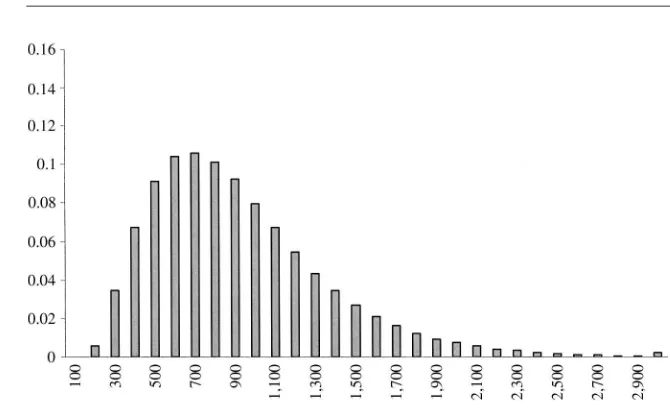
Figure 1
Observed (weighted) food expenditure for SFB data. 1,000 ⫽1million Italian Lira
excludes the top and bottom 1 percent of the per-capita food distribution. A first comparison reveals minor discrepancies for food consumption (SFB median is 10 percent below the corresponding SHIW statistic—the variance is instead lower in SHIW, and so is the overall range). The picture is quite different for nondurable expenditure: mean and median are much (20–25 percent) higher in SFB compared to SHIW; variability is also higher in SFB, as for food. The comparison looks promis-ing for income, but this might depend on heavy corrections to SFB data whose rec-ords are known to be based on total expenditure plus, where available, saving class information (see Brandolini 1999).
Inspection of Figures 2 and 4 reveals that SHIW expenditure data suffer from severe heaping and rounding problems (all expenditure figures are in thousands Ital-ian liras, where Lit 1,000 is approximately $0.5). For nondurable expenditure, there are spikes at all multiples of half a million (particularly at Lit 1, 1.5, 2, 2.5, 3 million); even though other spikes are found at Lit 0.8, 1.2, and 1.8 million. For food, there is a spike at Lit 1 million; smaller spikes also are found at Lit. 0.5, 1.5 and 2 million, even though all multiples of 0.1 million are well represented on the left of 0.9 million. The corresponding weighted histograms for SFB food and nondurable expenditure are presented in Figures 1 and 3.
Figure 2
Observed food expenditure for SHIW data. 1,000⫽1million Italian Lira
Figure 3
Figure 4
Observed nondurable expenditure for SHIW data. 1,000 ⫽1million Italian Lira
Figure 5
IV. A Theoretical Framework
In this section, we discuss the following identifying restriction to use SFB information to predict on SHIW
(1) E(lnC|X,SFB)⫽E(lnC|X,SHIW)
where Crepresents total nondurable consumption. This conditional independence property is known in the statistical econometric literature as (weak) ignorability as-sumption and represents a useful tool to account for observed heterogeneity between different units.
It implies that households with same (observable) characteristicsXhave (on aver-age) the same levels of (log) nondurable expenditure, no matter if they belong to the SFB or the SHIW sample. This also means that everything matters to explain heterogeneity of nondurable expenditure across households is the information con-tained in the setXthat is common to the two samples.
In what follows, we build on the following specification for the regression func-tions involved in Equation 1. LetX⫽[Z, lnF], whereZare household characteristics recorded in both surveys and F represents food expenditure for each household. In agreement with standard models of consumer behavior, consider the following within period inverse Engel curve relating total nondurable expenditure (the budget) to food and sociodemographic variables
(2) lnC⫽ΒZ⫹ψ(lnF)⫹v.
The functionψis unknown and assumed suitably smooth over the support of lnF.5 As argued above, we have reliable information to estimate the regression function of (log) nondurable expenditure on (log) food expenditure andZusing SFB data. This would allow us—under Condition 1—to use the best linear predictor of Equation 2 to impute nondurable expenditures on SHIW, exploiting the joint information on food expenditure and household characteristics observed in this sample.
However, we have seen that the SHIW observed measure of food is affected by severe rounding and heaping problems, so that the nonclassical error relationship between true and coarsened values—lnFand lnF* respectively—could cause se-vere bias in the imputation step. Indeed, let
(3) E(lnC|X*,I⫽SHIW)
be the imputation equation conditional on observed informationX*⫽[Z, lnF*]in the SHIW sample. SinceX≠X*, the ignorability assumption stated in Equation 1 fails to hold. To fix the ideas, in a fully nonparametric context we would match a household with X characteristics in the SFB sample to a Z-similar household in the SHIW sample declaring a ln F* level of expenditure. Since the observed measure could potentially differ from the true unobserved value, this would cause
mator.
By the law of iterated expectations, the regression function in Equation 3 also can be written as
(4) E
冦
E(lnC|X*, lnF,I⫽SHIW)冧
where the external expectation is taken with respect to the conditional distribution of lnFgivenX* in the SHIW sample. If we assume that lnF* is a surrogate of ln F, that is if lnCdoes not depend on lnF* given lnF, the specification (Equation 2) implies the following rule to predict on SHIW
(5) βZ⫹E(ψ(lnF)|X*,I⫽SHIW)
Under such assumption, error affected values of food expenditure are ‘‘less informa-tive’’ in predicting total nondurable expenditure than true unobserved values, in the sense that, conditional on lnF, lnF* does not contain any information on lnc. This corresponds to assuming nondifferential measurement error characterizing reported values of food expenditure (Carroll, Ruppert, and Stefanski 1995); see Bound, Brown, and Mathiowetz (2001) for a discussion on the implications of such assump-tion.
The last expression implies that to predict nondurable expenditure on SHIW we need to infer both (i) on the functional form ofψand (ii) on the coarsening mecha-nism leading to error affected measure for food SHIW consumption data, that is the conditional distribution of lnFgiven lnF* andZ. Section V deals with the last point while the relationship between total nondurable and food expenditure in Equation 2 is discussed in Battistin, Miniaci, and Weber (2003).
V. Accounting for Heaping and Rounding Errors
Following Heitjan and Rubin (1990), assume that the random vari-able of interestW(expenditure in our case) is distributed according to a densityf(w; ϑ) depending on the unknown parameterϑ. IfWwas available, inference aboutϑ could be drawn directly by standard methods.
Suppose instead we only observe a subset of the complete data sample space in which the true unobservable data lie. In other words, instead of observingWdirectly, we only observe a coarse versionW* of the variableW. Assume that the degree of coarseness can be summarized by a continuous random variable G, whose condi-tional distribution givenWdepends onγ, the parameter of the incompleteness mecha-nism. This means thatW* can always be expressed as a function of the pair (W, G). More formally, the conditional distribution ofW*, given the true unobserved value Wand the coarsening variableGis degenerate
(6) f(w*|w, g, z)⫽
冦
10 ififw*w*⫽≠W*(w, g)W*(w, g)(W, G) that are consistent with the valuew*. In what follows we assume that the variable Gis not directly observed, but can at best be inferred from the observed valuew*. The likelihood function for the parameters (ϑ,γ) in the SHIW sample can be written as
Moving from the evidence suggested by SHIW empirical distributions for both food and nondurables, we assume that households round off their true expenditure values to the nearest multiple of 100, 500, or 1,000 (denote these three error types asR1,R2, andR3, respectively) so that
w*∈R1⇒ |w⫺w*|ⱕ50,
(9) w*∈R2⇒ |w⫺w*|ⱕ250,
w*∈R3⇒ |w⫺w*|ⱕ500.
Assume that disjoint regions in the domain ofG uniquely correspond to different rounding errors, so that there exist two thresholdsτ2andτ1(τ2⬎τ1) withg ⱖτ2
We specify an ordered (three category) probit regression model for the conditional distribution ofGgivenWandZ
(12) f(g|w,z;γ)⬃N(γ1w⫹γ2z; 1)
Exploratory results based on a nonparametric estimation of the dou-ble log Engel curve using SFB data suggest that the relation between lnCand ln Fis close to being linear. The linearity is confirmed by semiparametric estimation conditional on demographics (see Battistin, Miniaci, and Weber 2003). We therefore write Equation 2 as
(13) lnC⫽βZ⫹αlnF⫹v
and estimate it by standard parameric regression methods.
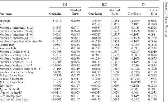
In Table 3, we present three sets of estimates of the last equation. The first set of numbers refers to parameter estimates and standard errors for a specification that linearly relates lnCto theZvariables but ignores any information about lnF(SM). The explanatory variables include region of residence, household composition indicators, education, sex, and age of the head and their interactions (zero-sum monthly dummies were also used, but their coefficients are not reported). Also in-cluded are some real wealth and standard of living indicators (home-ownership and the quality of housing available to the consumers, as proxied by the total surface of the dwelling and its per-capita surface). The fit of the equation is quite good (adjusted R2
⫽0.44).
The second set of numbers reports OLS estimates of the Inverse Engel Curve (IEC), thus including the information on food expenditure. The addition of this single regressor makes the fit of the equation improve dramatically (adjustedR2
⫽0.66), supporting the idea of including food information in the matching exercise. A reason for concern could be that we estimate the key parameter (the ln Fcoefficient) at 0.7362. This appears to imply that the elasticity of food expenditure to total nondura-ble expenditure is 1.36, an implausibly high number. However, OLS does not pro-duce a consistent estimate of the reciprocal of the budget elasticity of food for two reasons: First, the relation is estimated in inverse form; second, simultaneity implies that ln Fin Equation 2 correlates with the equation errorv.6
To check whether SFB consumption data are reliable, we also estimate the IEC by instrumental variables (IV); results are reported in the last set of numbers of Table 3. We treat lnFas endogenous and we use as additional instruments four variables capturing home ownership and quality of housing available to the consumers. The idea is that these variables correlate with the long-term standard of living the house-hold can afford. The fact that Engel curve estimation is a well-established practice in the economic literature helps us evaluate economically the success of our matching procedure (see for example Deaton and Muellbauer 1980 for further details on Engel curves and their economic interpretation). Even though the estimated standard er-rors of the estimates are larger, inference can still be drawn with good confidence.
Journal
of
Human
Resources
Engel Curve Estimates Using SFB Data
SM IEC IV
Standard Standard Standard
Parameters Coefficient Error Coefficient Error Coefficient Error
Intercept 5.8614 0.1050 2.2329 0.0854 ⫺4.7960 0.5026
lnF 0.7362 0.0051 2.1842 0.0979
Number of members 18–26 0.1345 0.0701 0.0967 0.0545 0.0185 0.1028 Number of members 27–40 0.1644 0.0678 0.0600 0.0527 ⫺0.1506 0.1003 Number of members 41–60 0.0930 0.0664 ⫺0.0027 0.0515 ⫺0.1931 0.0981 Number of members 61–70 ⫺0.0484 0.0661 ⫺0.0830 0.0513 ⫺0.1536 0.0968 Number of members older than 70 ⫺0.1310 0.0675 ⫺0.1226 0.0524 ⫺0.1093 0.0986 Central Italy ⫺0.0580 0.0455 ⫺0.0468 0:0354 ⫺0.0235 0.0666 Southern Italy ⫺0.1918 0.0370 ⫺0.1587 0.0288 ⫺0.0931 0.0544 Number of children 0–2 ⫺0.3668 0.0666 ⫺0.1496 0.0517 0.2847 0.1019 Number of children 3–5 ⫺0.2817 0.0694 ⫺0.1601 0.0539 0.0831 0.1028 Number of children 6–9 ⫺0.2780 0.0639 ⫺0.1284 0.0496 0.1670 0.0955 Number of children 10–13 ⫺0.1806 0.0666 ⫺0.0712 0.0517 0.1459 0.0984 Number of children 14–17 ⫺0.0406 0.0632 ⫺0.0083 0.0491 0.0586 0.0924 Number of children older than 18 0.1105 0.0319 0.0608 0.0247 ⫺0.0344 0.0470 Number of retired members 0.0598 0.0129 0.0497 0.0100 0.0306 0.0189 At least 2 members 0.7152 0.0337 0.1808 0.0265 ⫺0.9579 0.0832 At least 3 members ⫺12.1028 0.7911 ⫺3.1488 0.6176 16.0220 1.5905 At least 4 members 7.1227 0.6459 1.6569 0.5031 ⫺10.0636 1.1525 Sex (male) 0.0602 0.0127 ⫺0.0103 0.0099 ⫺0.1478 0.0208 Age of the head 0.0123 0.0027 0.0052 0.0021 ⫺0.0081 0.0041 (Age of the head)2
Battistin,
Miniaci,
and
Weber
369
South ∗number 18–26 ⫺0.1668 0.0439 ⫺0.0721 0.0341 0.1164 0.0655 Center∗number 27–40 ⫺0.0357 0.0520 0.0114 0.0404 0.1043 0.0764 South ∗number 27–40 ⫺0.1496 0.0431 ⫺0.0633 0.0334 0.1096 0.0639 Center∗number 41–60 ⫺0.0474 0.0469 0.0005 0.0364 0.0926 0.0690 South ∗number 41–60 ⫺0.1625 0.0387 ⫺0.0340 0.0301 0.2199 0.0590 Center∗number 61–70 ⫺0.0044 0.0443 0.0201 0.0344 0.0677 0.0649 South ∗number 61–70 ⫺0.1313 0.0362 ⫺0.0015 0.0281 0.2558 0.0555 Center∗number older than 701 ⫺0.0409 0.0474 0.0301 0.0368 0.1702 0.0700 South ∗number older than 70 ⫺0.1672 0.0392 ⫺0.0211 0.0305 0.2680 0.0605 Center∗educationⱖ8 ⫺0.0121 0.0193 ⫺0.0183 0.0150 ⫺0.0311 0.0282 Center∗educationⱖ13 0.0257 0.0203 0.0316 0.0157 0.0446 0.0296 Center∗degree 0.0092 0.0316 0.0154 0.0246 0.0289 0.0463 South ∗educationⱖ8 ⫺0.0104 0.0167 ⫺0.0013 0.0129 0.0144 0.0244 South ∗educationⱖ13 0.0341 0.0175 0.0342 0.0136 0.0350 0.0256 South ∗degree 0.0217 0.0277 0.0090 0.0215 ⫺0.0164 0.0406 Center∗sex 0.0270 0.0193 0.0076 0.0150 ⫺0.0308 0.0283
South ∗sex 0.0230 0.0174 0.0169 0.0135 0.0035 0.0254
Total surface 0.0023 0.0002 0.0012 0.0001 Per-capita surface 0.0008 0.0004 0.0010 0.0003
Homeowner 0.0315 0.0066 0.0273 0.0051
Secondary residence 0.2043 0.0120 0.1529 0.0093
Adjusted R2 0.4361 0.6598
F(58, 31341) 419.67
F(59, 31340) 1,033.32
F(55, 31344) 206.47
Root MSE 0.4901 0.3807 0.7169
The estimated elasticity of food is 0.46 and this is fully consistent with the well-documented notion that food is a necessity.7
VII. Estimates of the Heaping Process
The error mechanism derived in Section V allows us to account for the heaping problems characterizing food and nondurable expenditures in the SHIW sample using predictive means derived from a fully parametric imputation model.
Exploratory plots of both lnCand lnFon the components ofZin the SFB sample suggest that a gaussian parametric specification for the conditional densities is plau-sible
(14) f(w|z;ϑ)⬃N(ϑ1z;ϑ2)
Exploiting the notation of Section V, we therefore assume that the joint distributions (lnC,G)|Z and (lnF,G)|Zare both bivariate normals and specify the likelihood function (Equation 8) accordingly.8
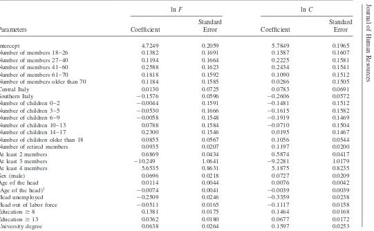
The conditioning set Z includes the same household characteristics described in Section III, plus a reasonable set of interview quality indicators (such as inter-view length and interinter-viewer’s assessment on how well the respondent understood the questions), which we assume not to determine consumption level. For com-putational convenience, we also impose the exclusion restriction that the rounding processGis a function of a limited number of exogenous characteristics (namely, age, education, and region). It is in fact possible that response care depends on both recall ability and the shadow value of leisure, which will differ across house-holds.
In Table 4, we present maximum likelihood estimates of ϑ for SHIW food and nondurable expenditure together with estimates of the parameter γ in the heaping function. The adopted specification for the heaping function (Equation 12) allows us to establish that we cannot ignore the stochastic nature of the coarsen-ing mechanism in drawcoarsen-ing inferences about the parameter ϑ. Maximum likeli-hood estimates of the parameter γ support the idea that the reported expenditure is not coarsened at random.9 We find that for food a lower expenditure level in-creases the probability of rounding to multiples of 1,000 (γ1is positive and
signifi-7. A reassuring feature of this set of estimates is that the estimated direct Engel curve also implies elastici-ties for food of approximately 0.45. This can be taken as evidence that our sample is sufficiently large for us to rely on asymptotic properties of the estimator (IV is not invariant to normalization in finite samples).
8. The integration setsH1,H2, andH3are[ln(w*⫺500), ln (w*⫹500)),[ln(w*⫺250), ln(w*⫹250)),
and[ln(w*⫺50), ln(w*⫹50)), respectively, whereW*⫽C* (observed nondurable expenditure) or W*⫽F* (observed food expenditure).
more likely to multiples of 100. For nondurable consumption, instead, rounding er-rors to multiples of 1,000 are associated with high expenditure levels and short inter-views.
We create multiple imputations of lnCand lnFfor the SHIW sample implement-ing an acceptance-rejection procedure based on the fitted model. Since by applyimplement-ing Bayes theorem we have
(15) f(w, g|w*,z;ϑ,γ)⬀
冦
f(w,g|z;0 ϑ,γ) ififw*w*⫽≠W*(w,W*(w,g)g)for each unit, we draw a couple (W, G) from the estimated distributionf(w, g|z;ϑ, γ) until (w, g) ∈ H(w*), that is, until the generated couple is consistent with the observed valuew*. We then imputeWas the true value of the observed (food or nondurable) expenditure. The proportion of missing values—that is the proportion of couples not consistent with observed expenditures—using 1,000 drawings from the estimated distributions is always less than 1 percent.10
Validating generated values for lnCand lnFusing SFB data helps us to conclude that food data are of comparable quality and information content across the two surveys, once heaping and rounding are accounted for. A different conclusion must be drawn for nondurable expenditure. Average histograms of 100 imputations are shown in Figures 6 and 7 and can be compared to the corresponding distributions of food and nondurable expenditure for the SFB sample (Figures 1 and 3). Different composition with respect to observable characteristics is corrected by weighting SFB observations to obtain the same distribution of observable characteristics for the two samples.
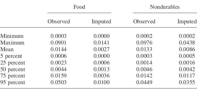
To assess the effectiveness of the error correction procedure, Table 5 reports descriptive statistics for the absolute differences between the SFB empirical and the SHIW estimated density functions, both for ln C and ln F. For the food measure, the imputation procedure fails to recover the lower tail of the distribu-tion but is globally close to the one observed for the SFB sample (differences be-tween histograms shift significantly toward zero with a mean reduction of about 80 percent). Instead, the SHIW empirical distribution for nondurable expendi-ture is based on much lower values than the SFB one and lies at its left. The underre-porting pattern showed in Table 2 is not accounted for by the heaping process alone.
Journal
of
Human
Resources
Heaping Correction for SHIW Data
lnF lnC
Standard Standard
Parameters Coefficient Error Coefficient Error
Intercept 4.7249 0.2059 5.7849 0.1965
Number of members 18–26 0.1382 0.1691 0.1587 0.1607
Number of members 27–40 0.1194 0.1664 0.2225 0.1581
Number of members 41–60 0.2588 0.1623 0.2434 0.1541
Number of members 61–70 0.1818 0.1592 0.1090 0.1512
Number of members older than 70 0.1184 0.1585 0.0286 0.1505
Central Italy 0.0130 0.0725 0.0783 0.0691
Southern Italy ⫺0.1576 0.0596 ⫺0.2606 0.0572
Number of children 0–2 ⫺0.0044 0.1591 ⫺0.1481 0.1512
Number of children 3–5 ⫺0.0530 0.1666 ⫺0.1615 0.1582
Number of children 6–9 ⫺0.0058 0.1548 ⫺0.1919 0.1469
Number of children 10–13 0.0788 0.1584 ⫺0.0710 0.1504
Number of children 14–17 0.2300 0.1546 0.0195 0.1467
Number of children older than 18 0.0855 0.0567 0.1056 0.0544
Number of retired members 0.0935 0.0207 0.1197 0.0200
At least 2 members 0.6869 0.0434 0.5874 0.0417
At least 3 members ⫺10.249 1.0641 ⫺9.2281 1.0179
At least 4 members 5.6535 0.8631 5.1875 0.8235
Sex (male) 0.0696 0.0218 0.0727 0.0209
Age of the head 0.0114 0.0044 0.0076 0.0042
(Age of the head)2 ⫺0.0074 0.0041 ⫺0.0039 0.0039
Head unemployed ⫺0.2509 0.0246 ⫺0.3359 0.0238
Head out of labor force ⫺0.0511 0.0165 ⫺0.1117 0.0158
Educationⱖ8 0.1381 0.0175 0.1464 0.0168
Educationⱖ13 0.0362 0.0180 0.0677 0.0172
Battistin,
Miniaci,
and
Weber
373
Center∗number 41–60 0.0494 0.0855 ⫺0.1683 0.0814
South∗number 41–60 ⫺0.0745 0.0694 ⫺0.1784 0.0666
Center∗number 61–70 0.1019 0.0881 ⫺0.1410 0.0840
South∗number 61–70 0.1611 0.0731 ⫺0.0058 0.0701
Center∗number older than 70 0.0555 0.0753 ⫺0.0633 0.0718
South∗number older than 70 0.0134 0.0624 ⫺0.0196 0.0600
Center∗educationⱖ8 ⫺0.0384 0.0703 ⫺0.0973 0.0670
Center∗educationⱖ13 0.0766 0.0573 0.0379 0.0550
Center∗degree 0.0957 0.0739 ⫺0.0268 0.0705
South∗educationⱖ8 0.1200 0.0624 0.1296 0.0599
South∗educationⱖ13 ⫺0.0702 0.0312 ⫺0.0119 0.0298
South∗degree 0.0313 0.0317 0.0123 0.0302
Center∗sex ⫺0.0158 0.0497 ⫺0.0075 0.0473
South∗sex ⫺0.0237 0.0261 ⫺0.0087 0.0251
Total surface 0.0871 0.0280 0.1142 0.0268
Per-capita surface 0.1239 0.0418 0.1004 0.0399
Homeowner ⫺0.0426 0.0324 ⫺0.0630 0.0310
Secondary residence ⫺0.0192 0.0280 ⫺0.0124 0.0271
lnϑ2 ⫺0.9920 0.0087 ⫺1.0469 0.0114
γ1 1.7659 0.0831 ⫺0.3195 0.0573
Fair understanding 0.0498 0.1017 0.1896 0.0626
Good understanding ⫺0.0172 0.0906 0.3808 0.0570
Excellent understanding 0.1964 0.0936 0.6866 0.0607
Long interview (over 1 hour) ⫺0.0402 0.0571 0.2959 0.0376
Age⬎70 ⫺0.1031 0.1086 ⫺0.4243 0.0616
τ2 17.779 1.5654 ⫺0.9110 0.4455
Figure 6
Imputed food expenditure for SHIW data. 1,000⫽1 million Italian Lira.
Figure 7
Imputations
5 percent 0.0006 0.0000 0.0003 0.0005
25 percent 0.0023 0.0006 0.0014 0.0016
50 percent 0.0044 0.0013 0.0046 0.0042
75 percent 0.0159 0.0036 0.0142 0.0117
95 percent 0.0503 0.0100 0.0449 0.0355
VIII. Prediction Results
Before commenting on the estimation results, it is worth summariz-ing the steps we have followed to impute alternative measures of nondurable con-sumption for the SHIW sample. We at first have argued that SFB data contain reliable information on expenditure items; we have then constructed food and total nondura-ble expenditure aggregates that are diary-based and are defined in a way that is fully comparable to SHIW corresponding items. In addition, we have seen that an inverse Engel curve can be successfully estimated exploiting such data.
Hence, exploiting SFB as validation data for the consumption information, we have shown that the type of rounding and heaping errors characterizing SHIW can be dealt with in estimation. In particular, the underlying density function is compara-ble for food expenditure, but differs markedly for total nonduracompara-ble expenditure.
We therefore present three alternative estimates ofE(lnC) for the SHIW sample. The first one builds on error-corrected values for ln Cexploiting results from the multiple imputation procedure described in the previous section. The effectiveness of this correction has already been discussed in Table 5. The second correction we propose builds on IEC prediction by means of the error corrected values for lnF generated in the SHIW sample. The third one neglects information on food expendi-ture—thus imposingα⫽0 in Equation 13—and is therefore both robust to potential misspecification in the multiple imputation procedure and unaffected by imputation variability.
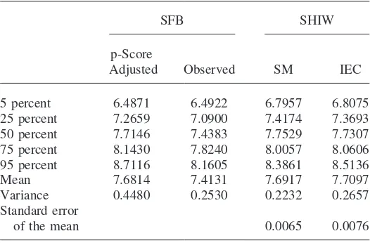
Table 6
Descriptive statistics for In(non durables)
SFB SHIW
p-Score
Adjusted Observed SM IEC
5 percent 6.4871 6.4922 6.7957 6.8075
25 percent 7.2659 7.0900 7.4174 7.3693 50 percent 7.7146 7.4383 7.7529 7.7307 75 percent 8.1430 7.8240 8.0057 8.0606 95 percent 8.7116 8.1605 8.3861 8.5136
Mean 7.6814 7.4131 7.6917 7.7097
Variance 0.4480 0.2530 0.2232 0.2657
Standard error
of the mean 0.0065 0.0076
A. Consumption Profiles
Given the results presented in Table 5, we resort to the SM and the IEC methods to impute nondurable expenditure in the SHIW sample. Table 6 reports the distribu-tions of nondurable consumption (in logs) based upon observed and predicted values. The table reveals that both mean and median lnCare higher in the SFB sample (after allowance is made for sampling differences) compared to the SHIW sample observed data, as we already pointed out. After correction, these differences all but disappear: median consumption (in logs) is now 2–4 percent higher in the SHIW sample, while mean consumption is again 1–2 percent higher. The variance is much higher in SFB than in SHIW (44.8 percent as opposed to 25.3 percent); SM predic-tions have lower variance (22.3 percent) while IEC imputapredic-tions display some more variability (26.6 percent). A similar picture emerges when we consider interquartile differences.11
Table 6 also reports standard errors for the mean prediction of lnC, based upon prediction error variances. The SM prediction error variance is the sum of the vari-ance of the disturbvari-ance and the varivari-ance of the parameter estimates, as usual. With the IEC method—thus conditional upon Zand lnF—a third variance component comes into play, reflecting the variability induced by the imputation procedure (see Battistin, Miniaci, and Weber 2003, for further details). The standard errors are of comparable magnitude, but the IEC standard error is larger than the SM standard error, indicating that imputation variance is of nonnegligible magnitude.
Figure 8 presents age profiles for consumption corresponding to the last three
Figure 8
Predicted and actual ln C age profiles
columns of Table 6: observed consumption, SM predictions and IEC predictions.12 All 100 IEC predictions are shown as individual points, to highlight the variability in the predicted profile that is attributable to the imputation method (there are 100 food imputations per household, and thus 100 lnCprofiles). The solid line passing through these points is the median IEC profile.
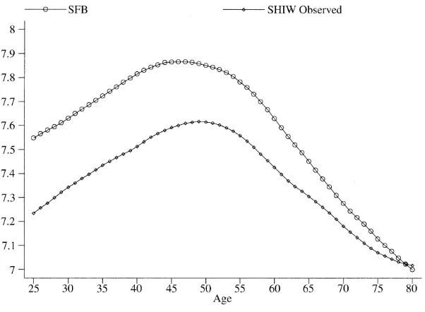
As previously noted looking at the overall sample, both the SM and the IEC pro-files are markedly above the observed profile, so that their level is of magnitude similar to the one observed for SFB (see Figure 5).13Their shape remains basically the same between ages 42 and 56, but is different outside this interval. We notice that the key difference between the two lies in the shape for households aged younger than 35 and older than 60: the inverse IEC method predicts a sharper rise early in life and a much smaller fall in old age than the standard method.
The question remains whether these profiles are statistically different. This re-quires computing the confidence interval of the difference, something that is most easily done by bootstrapping methods. (The variance of the difference is not simply the sum of the variances here. Given that we predict over the same sample using at least some common information, the prediction errors are positively correlated.) In Figure 9, we report the difference between SM and IEC saving age profiles together with the corresponding bootstrap confidence bands of⫾2 standard errors. We can
12. The age profile based on the measure of lnCderived from the heaping correction of Section VII is extremely close to the observed profile, and therefore is not reported. The profile of observed data is the one already reported in Figure 5.
Figure 9
Difference in predicted ln C profiles and confidence interval
see the two profiles are statistically different over most of the age range, with the notable exception of some ages in the 45–55 interval.
B. Saving profiles
Much of the literature on savings is interested in the age profile of the saving rate, as the leading economic theory (the life-cycle model of consumption) predicts a hump-shaped age profile for individual households, with negative savings past retire-ment age. It is well known that cross-section profiles do not correct for cohort effects, and therefore may provide a misleading picture of the true underlying age profile for each cohort. The cross-section plot of our different measures still may be interesting, however, if we believe cohort effects to be zero for the saving rate (as assumed by Paxson 1996) or unaffected in imputation.
The existing evidence for Italy conflicts with the theoretical predictions. As dis-cussed in Section II, SHIW saving rates are high and positive at all ages and rising until at least age 60, that is past retirement age (statutory retirement age was 60 for men and 55 for women in 1995, but in our sample about a third of male heads have already retired by age 55). Cross-section financial wealth profiles show a peak after age 60, possibly related to the large lump-sum payment that employees receive when they retire. Average wealth holdings then decline until age 75, when they rise again. Evidence on financial wealth is presented in Brugiavini and Padula (2003), who use SHIW, and in Miniaci and Weber (2002), who instead use data from the recently released Survey on Health, Aging and Wealth, SHAW. To interpret this evidence we must be careful, because cohort effects and differential mortality by wealth are likely to play an important role with financial wealth.
af-Figure 10
Relation between entropy and variance of ln C
fects the saving rate age profile, once we also correct for possible measurement error problems with the available income data.
The standard definition of the personal sector saving rate in aggregate data is given by 1 ⫺total consumption/income where income refers to disposable income and total consumption is either the sum of spending on durable goods and nondurable goods and services, or just expenditure on nondurable goods and services. Note that in both cases, contrary to the definition of consumption we followed to derive lnC in the previous section, consumption includes rent (that we observe in SHIW).
If we wish to produce evidence on a saving rate definition that is comparable to the aggregate measure, we need to generate predictions for the levels. To do this, we can resort to the following relationship between moments of logs and levels
(16) lnE(C)⫺E(lnC)⫽1
2Var (lnC)
that holds true if lnCis normally distributed. In Section VII, we have already used the fact that such an assumption is reasonable in our data. Indeed, Figure 10 reports the left hand side—sometimes referred to as entropy—and the right hand side of Equation 16 against age for SFB data.14We see that the difference is minor for all ages and does not display a strong age pattern.
A close approximation for the first moment of C at any age can therefore be obtained as
(17) E(C)⫽exp
冢
E(lnC)⫹12Var(lnC)
冣
This can be used to generate predictions for the first moment of Cin the SHIW sample if we replace the unobserved first and second moments of lnCwith their consistent estimates.15
This approximation allows us to compute average spending by age in the SHIW sample. We alternatively define spending as (i) the sum ofCand rent, that is treating spending on durable goods as saving, and (ii) the sum ofC, rent and durables, that is, treating spending on durables as consumption. Given that we base our estimates for expenditure on SFB information and the same information is used to generate aggregate statistics for the NIPA, we expect our consumption data to be in line with the corresponding NIPA aggregate.
To compute a measure of saving, we also need an estimate of average income by age that is consistent with the NIPA figure. Income is poorly measured in SFB as responses are based on a single question about normal monthly income, and (see Brandolini 1999) in some 40 percent of cases the SFB figure has been revised upward by exploiting information on total expenditure (plus, where available, saving class information). SHIW contains a number of detailed questions on income and is there-fore a more promising source of information. We know from Brandolini (1999), however, that in 1995 SHIW income data fell short of national accounts estimates by 34.7 percent; thus we could produce a grossed-up income profile by multiplying each household’s income by 1/(1⫺.347)⫽1.53. More important, Brandolini pro-vides information on proportional shortfalls by income type: for employment in-come, this is 18.4 percent, while for transfer income (including pensions) it rises to 25.7 percent. The larger shortfall in transfer income compared to employment in-come is to some extent surprising, and may reflect failure to report secondary trans-fers (such as invalidity pensions and supplementary occupational pensions) rather than primary pensions.16The SHIW is found to overestimate the rent component of income compared to the National Accounts by 10.6 percent. Severe underestimation affects instead interest income (80.1 percent) and self-employment income (63.8 percent).
Underestimation of interest income is common in household surveys, and its cor-rection is relatively straightforward and of little consequence for the income age profile in our data. The underestimation of self-employment income is also relatively common, but the size of the required correction (the grossing-up factor is 2.76 in
15. For the first moment, we take the SHIW sample mean of the imputed lnC. The variance of lnCis instead estimated as the sum of the SHIW sample variance of the imputed lnCand the variance of the residuals from the regressions in Table 4. An alternative, equivalent estimator is given by the SFB sampling variance of the observed lnC.
Figure 11
Saving Rate—consumption includes durables
this case) and its application to a relatively small subsample (in SHIW only 18.2 percent of all households can be classified as self-employed) produces major differ-ences between corrected and original income age profiles.
However, there are good reasons to doubt the grossing-up procedure; first, because the NIPA statistic is at best an educated guess and secondly because the correction falls heavily on too small a number of households (unit nonresponse in SHIW ap-pears to be higher among the self-employed). For this reason we compute the saving rate age profiles for that part of the SHIW sample that excludes the self-employed households (defined as those households where the head is self-employed or at least a fourth of reported household income is from self-employment). In Figure 11 we show the saving rate age profile corresponding to the standard NIPA aggregate, thus treating spending on durable goods as consumption. The income measure is corrected using the grossing-up factors described above. The top line corresponds to reported expenditure (‘‘observed’’) and rises from values around 25 percent for young house-holds to values in the 45 percent region around age 65 (statutory retirement age was 60 in 1995 for males, 55 for females). After that age, the saving rate profile flattens out. The same statistic taken over the whole sample is 43.4 percent.
Figure 12
Saving Rate—no durables spending in consumption
age corresponding to the 100 food imputations per household using the IEC method. The median profile makes up the third line and we take it as representing the IEC age profile. Such line is still monotonically increasing, albeit with a lower slope than the one corresponding to the SM method (from 5 percent at 25 to 35 percent at 80 years of age). Its overall value is 24.6 percent.
To understand these findings we can go back to Figure 5. This shows that the SFB age profile of nondurable consumption lies all above the corresponding SHIW profile, but the SHIW profile falls more gently with age. The former feature accounts for the higher level of the saving rate based on observed SHIW consumption; the second feature for its less steep ascent with age compared to the standard method predictions. The IEC method further exploits SHIW information on food consump-tion and therefore does not generate as steeply decreasing consumpconsump-tion levels in old age as the standard method (see Figure 8 for similar evidence on lnC).
In this paper we compare food and nondurable expenditure data across two Italian surveys: the widely used, recall-questions-based Survey of House-hold Income and Wealth (SHIW) and the newly released diary-based Survey of Fam-ily Budgets (SFB). The former contains detailed income and wealth information, but only a few, broad consumption questions; the latter contains accurate records on consumption, but little (if any) income and no wealth information. The two sur-veys share information on social and demographic household characteristics.
We have argued that the consumption data in SHIW are questionable because of the nonstandard nature of recall measurement error and that a matching technique should be used to generate predictions for total nondurable expenditure in SHIW.
In a first step, we have analysed the nature of the recall error process. When we compare marginal densities for food expenditure and total nondurable expenditure, modeling the heaping and rounding process as a function of interview quality infor-mation, observed characteristics, and the true expenditure level, we find that:
• the SHIW reported food expenditure measure is comparable to the SFB mea-sure once heaping and rounding errors are taken into account
• the SHIW reported nondurable expenditure measure is instead more seriously affected by recall error.
Based on the above, we have argued that it makes sense to use inverse Engel curve estimates from the SFB to generate an imputation for nondurable expenditure in SHIW. In a second step, we therefore estimate a double-log inverse Engel curve and show that parameter estimates agree well with standard findings on consumer behavior.
We then discuss the relative merits of two prediction techniques: the standard method (SM) that makes no use of food information in the SFB sample and an Inverse Engel Curve (IEC) method that uses food records from both SFB and SHIW samples. This latter method exploits information on reduced form variables and from imputations on SHIW food consumption that is consistent with the estimated heaping and rounding process. Even though more information is used in estimation, the over-all precision of the IEC predictions is potentiover-ally reduced because of imputation errors.
aggregate saving rate measure, but an even more steeply ascending age profile. The inverse Engel curve method also produces a reasonable aggregate measure, but an age profile that increases less steeply with age than the profile of the standard predic-tion method. In all cases, however, there is strong evidence of active saving behavior after retirement.
References
Ando, Albert, Luigi Guiso, and Ignazio Visco, eds. 1994.Saving and the Accumulation of Wealth. Essays on Italian Households and Government Saving Behavior. Cambridge: Cambridge University Press.
Angrist, Joshua, and Alan Krueger. 1992. ‘‘The Effect of Age at School Entry on Educa-tional Attainment: An Application of Instrumental Variables with Moments from Two Samples.’’Journal of the American Statistical Association87(418):328–36.
Arellano, Manuel, and Costas Meghir. 1992. ‘‘Female Labor Supply and On-the-Job Search: An Empirical Model Estimated Using Complementary Data Sets.’’Review of Economic Studies59(3):537–57.
Attanasio, Orazio, and Guglielmo Weber. 1993. ‘‘Consumption Growth, the Interest Rate and Aggregation.’’Review of Economic Studies60(3):631–49.
Banca d’Italia. 1999.Annual Report for 1998(Relazione del Governatore 1998). Rome: Banca d’Italia (available at http://www.bancaditalia.it).
Banks, James, Richard Blundell, and Sarah Tanner. 1998. ‘‘Is There a Retirement-Savings Puzzle?’’American Economic Review88(4):769–88.
Battistin, Erich. 2002 ‘‘Errors in Survey Reports of Consumption Expenditures.’’ London: Institute for Fiscal Studies. Mimeo.
Battistin, Erich, Raffaele Miniaci, and Guglielmo Weber. 2003. ‘‘What Do We Learn from Recall Consumption Data?’’ Tema di Discussione n.466. (previously: WP10/00, Lon-don: Institute for Fiscal Studies).
Bound, John, Charles Brown, and Nancy Mathiowetz. 2001. ‘‘Measurement Error in Sur-vey Data.’’ InHandbook of Econometrics, Volume 5, ed. James Heckman and Eduard Leamer, 3707–3843. Amsterdam: North-Holland.
Brandolini, Andrea. 1999. ‘‘The Personal Distribution of Incomes in Post-War Italy: Source Description, Data Quality and the Time Pattern of Income Inequality.’’Giornale degli Economisti58(2):182–39.
Brandolini, Andrea, and Luigi Cannari. 1994. ‘‘Methodological Appendix: The Bank of Ita-ly’s Survey of Household Income and Wealth.’’ InSaving and the Accumulation of Wealth. Essays on Italian Households and Government Saving Behavior, ed. Albert Ando, Luigi Guiso, and Ignazio Visco, 369–86. Cambridge: Cambridge University Press.
Brugiavini, Agar, and Mario Padula. 2001. ‘‘Too Much for Retirement? Saving in Italy.’’
Research in Economics55(1):39–60.
———. 2003. ‘‘Household Saving Behavior and Pension Policies in Italy.’’ InLife-Cycle Savings and Public Policy: A Cross-National Study in Six Countries, ed. Axel Boersch-Supan, 101–47. Academic Press.
Carrol, Raymond, David Ruppert, and Leonard Stefanski. 1995.Measurement Error in Nonlinear Models. London: Chapman and Hall.
bridge: Cambridge University Press.
Guiso, Luigi, Tullio Jappelli, and Daniele Terlizzese. 1992. ‘‘Earnings Uncertainty and Pre-cautionary Saving.’’Journal of Monetary Economics30(2):307–37.
———. 1996. ‘‘Income Risk, Borrowing Constraints and Portfolio Choice.’’American Economic Review86(1):158–72.
Heckman, James, Hidehiko Ichimura, Jeff Smith, and Petra Todd. 1998. ‘‘Characterizing Selection Bias Using Experimental Data.’’Econometrica66(5):1017–98.
Heitjan, Daniel, and Donald Rubin. 1990. ‘‘Inference from Coarse Data via Multiple Impu-tation with Application to Age Heaping.’’Journal of the American Statistical Associa-tion85(410):304–14.
———. 1991. ‘‘Ignorability and Coarse Data.’’The Annals of Statistics19(4):2244–53. Little, Rod, and Donald Rubin. 1987.Statistical Analysis with Missing Data. New York:
Wiley.
Miniaci, Raffaele, and Guglielmo Weber. 2002. ‘‘The Wealth Accumulation of Italian Households: Evidence from SHAW.’’ Padova: Universita` di Padova, Department of Eco-nomics. Mimeo.
Paxson, Christina. 1996 ‘‘Saving and Growth: Evidence from Micro Data.’’European Eco-nomic Review40(2):255–88.
Pischke, Jorn-Steffen. 1995. ‘‘Measurement Error and Earnings Dynamics: Some Estimates from the PSID Validation Study.’’Journal of Business&Economic Statistics13(3): 305–14.
Pistaferri, Luigi. 2001. ‘‘Superior Information, Income Shocks and the Permanent Income Hypothesis.’’Review of Economics and Statistics83(3):465–76.
Rosati, Nicoletta. 1999. ‘‘Matching statistico tra dati Istat sui consumi e dati Bankitalia sui redditi per il 1995.’’ Discussion Paper no. 7. Padova: Universita` di Padova, Department of Economics.
Rosenbaum, Paul, and Donald Rubin. 1983. ‘‘The Central Role of the Propensity Score in Observational Studies for Causal Effects.’’Biometrika70(1):41–55.