Education, and the High School
Dropout Decision
Kelly Foley
Giovanni Gallipoli
David A. Green
Foley, Gallipoli, and Greenabstract
The probability of dropping out of high school varies considerably with parental education. Using a rich Canadian panel data set, we examine the channels determining this socioeconomic status effect. We estimate an extended version of Carneiro, Hansen and Heckman (2003)’s factor model, incorporating effects from cognitive and noncognitive ability and parental valuation of education (PVE). We fi nd that cognitive ability and PVE have substantial impacts on dropping out and that parental education has little direct effect on dropping out after controlling for these factors. Our results confi rm the importance of determinants of ability by age 15 but also indicate an important role for PVE during teenage years.
I. Introduction
In this paper we investigate the forces determining the high school dropout decision using a rich panel data set that includes survey responses from chil-dren, parents, and high school administrators. Following recent work by Heckman, Stixrud, and Urzua (2006); Cunha and Heckman (2007, 2008); and Cunha, Heckman, and Schennach (2010)—hereafter, HSU, CH07, CH08, and CHS, respectively—we use a factor based model to capture the effects of pre- high school skill investments as refl ected in cognitive and noncognitive ability measures. Our work confi rms their
fi ndings of the importance of these abilities (and the investments they refl ect), but it
Kelly Foley is an assistant professor of economics at the University of Saskatchewan. Giovanni Gallipoli is an associate professor of economics at the University of British Columbia. David Green is a professor of economics at the University of British Columbia. The authors thank participants at the Conference on Structural Models of the Labour Market and Policy Analysis, and the CLSRN and IRP workshops at the University of Toronto and University of Wisconsin, respectively, for their comments. The data used in this article can be obtained from the authors beginning May 2015 through April 2018.
[Submitted April 2012; accepted September 2013]
also identifi es and measures the effects on dropping out of a third unobserved factor: parental valuation of education.
The idea that how much parents value education—either in terms of its intrinsic worth or in terms of their perceptions of the economic returns—affects their children’s educational outcomes is neither surprising nor new. Parental aspirations for their chil-dren’s education were seen to be a key factor of the “Wisconsin Model” of educational attainment developed in the 1960s, ’70s and ’80s (Davies and Kandel 1981). Recent work by Attanasio and Kaufmann (2009) and CHS also suggests that parental expec-tations and infl uences have a nonnegligible effect on early education decisions. We provide further evidence that parental aspirations are strongly correlated with drop-ping out of high school. However, the interpretation of these results is complicated. Parents’ answers to questions (such as we use) about the level of education they “hope” their child will attain could refl ect their own valuation of education in general, an assessment of their child’s own capabilities, or some combination of the two. If they refl ect the former, this would call for policy responses that can substitute for parental and family infl uences. If, instead, the answers refl ect insider knowledge about a child’s own abilities, then policies should focus on how to generate those abilities in the fi rst place. We address this central identifi cation problem using a factor- model approach and provide a clear statement of the conditions under which our estimator permits identifi cation of the causal impact of parental valuations on children’s dropping out. In particular, we show that under a standard index suffi ciency condition, estimates of parental valuation effects, conditioning on a child’s existing stock of cognitive and noncognitive skills at age 15, can be interpreted as a direct impact during the teenage years. Specifi cally, the suffi ciency condition requires that the dropout decision de-pends only on the cognitive and noncognitive skill index values at age 15, not on how those values were generated. In this sense, our work is complementary to Todd and Wolpin (2006), CH07, and CHS, which focus on the dynamic production of cognitive and noncognitive skills up to age 14.
One key feature in data on dropping out of high school is the strong correlation between family socioeconomic status and dropping out (for example, Eckstein and Wolpin 1999; Belley, Frenette, and Lochner 2008, for the United States and Canada respectively). In Canadian data, described below, teenage boys with two parents who are themselves high school dropouts have a 16 percent chance of dropping out, com-pared to a dropout rate of less than 1 percent for boys whose parents both have a university degree. Because of this, we implement a factor model that incorporates
fl exibility in parental education effects. More specifi cally, we implement a fl exible version of the factor model presented by Carneiro, Hansen, and Heckman (2003)— hereafter, CHH—in which we explicitly account for nonlinearities in skill production by allowing the distributions of skills and parental valuations to vary in shape, as well as location, with parental education. Nonlinearities may refl ect socioeconomic differ-ences in endowments and investments, meaning that teenagers from highly educated families and those from less- educated families may be drawing from different ability and parental valuation distributions.
two years thereafter. The key dependent variable is whether the child is a high school dropout (that is, is no longer in school and has not graduated) at age 19. We focus on the high school dropout decision partly because it has important implications for lifetime outcomes of youth (see, for example, Campolieti, Fang, and Gunderson 2009) and partly because, with a negligible direct cost of staying in high school, it allows us to focus on issues other than short- term liquidity constraints. The latter are central to discussions of educational choices beyond high school but their presence may obscure investigation of other factors, particularly relating to parental infl uences, that are more cleanly isolated in our context. As we will see, family income has very small direct impact on dropping out of high school.
The YITS also includes surveys of a parent and of a school administrator when the child is 15. It contains a long list of questions related to individual characteristics often seen as refl ecting noncognitive abilities, as well as questions related to peers, the home environment, and aspirations. Factor models provide an ideal vehicle for examining data of this type, which consist of many noisy measures of individual characteristics. We set out a system containing a dropout indicator function augmented by a set of measurement equations related to key underlying factors, interpreted as the stock of pre- existing abilities (both cognitive and noncognitive) and parental valuation of edu-cation. The parental valuation factor is constructed to be correlated with measures of parental aspirations for their children’s education and their willingness to save for that education after controlling for family income level. Thus, it is a factor related to paren-tal valuation of education as revealed in parenparen-tal statements and actions. Identifi cation of the impacts of the factors in this class of models is obtained through covariance restrictions. We begin our investigation with a simple model of the dropping- out deci-sion that allows us to describe and defend our identifying restrictions.
We fi nd that the highest ability students are predicted never to drop out regard-less of parental education or parental valuation of education. However, for teenagers with medium and low cognitive ability, family background plays an important role in explaining their dropout decisions. For the least skilled children with parents who are themselves high school dropouts, whether their parents value education or not makes a strong difference in their chances of dropping out. A low cognitive- ability teenager whose parents are high school dropouts has a probability of dropping out of 0.045 if his parents place a high value on education, and 0.40 if his parents’ valuation of education is low. Interestingly, when parents place a high value on their less- skilled children’s education, we fi nd that parents’ own education level does not affect drop-ping out. Thus, differences in dropdrop-ping out by parental education status arise because families with diverse education backgrounds have different distributions of abilities and of parental valuation of education. Interpreted within our factor model, this is evidence that parental education does not have a direct effect on dropping out during the teenage years, though it could still play a role in developing cognitive and noncog-nitive abilities up to age 15.
II. Previous Literature
Our paper fi ts within a rich literature examining the high school drop-out decision, particularly for the US. In papers dating back to the 1960s, researchers developed variants of what came to be called the “Wisconsin Model” of educational and occupational attainment (Sewell, Haller, and Portes 1969; Alexander, Eckland, and Griffi n 1975; Haveman, Wolfe, and Spaulding 1991). A key element of this model was its emphasis on the development of educational aspirations during adolescence and the importance of parents and peers in shaping those aspirations. Parental aspira-tions for their children were seen to be of particular importance (see, for example, Davies and Kandel 2008).
Within the more recent economics literature, Eckstein and Wolpin (1999) uses a structural dynamic choice framework to examine dropping out in the Unites States. It fi nds that dropouts have lower ability and motivation as well as lower expectations about rewards from graduation. Todd and Wolpin (2006) investigates the form of the production function for cognitive skills using data from the NLSY79 Children Sample, focusing on implications for racial gaps in test scores. It fi nds that mother’s ability (as measured by the AFQT test) has a large impact on test score outcomes. Oreopoulos, Page, and Stevens (2006) fi nds that increases in parental education, stemming from changes in compulsory school laws in the Unites States, result in reduced dropping out for their children, though Black, Devereux, and Salvanes (2005) fi nds only limited evidence of such effects in Norwegian data.
Several papers fi nd an association between parental education and time and money inputs into children’s education and then between those inputs and children’s edu-cational outcomes. Carneiro et al. (2013) fi nds a causal impact of increased parental education on time inputs such as time spent reading to a child and whether the child has been taken to a museum. Haveman, Wolfe, and Spaulding (1991) and Del Boca, Flinn, and Wiswall (2014) argue that more time spent with a child, particularly when the child is young, improves educational outcomes.
Our paper contributes to this literature by focusing on the unobserved channels through which socioeconomic status operates. We distinguish between parental edu-cational plans for a specifi c child (which partly refl ects their assessment of the child’s abilities) and parents’ valuation of education in general. Thus, parents may generally value education very highly while also having low aspirations for what a child will achieve because they believe that child has low abilities. This distinction means that we can, under certain assumptions, test whether parents’ education and the value they place on their children’s education have a direct effect on children’s behaviour during their teenage years. Under our approach, increased parental time inputs are a refl ection of parental valuation of education.
III. Determinants of Dropping Out
A. Model Outline
are estimating and how to achieve identifi cation. Before describing the model it is helpful to briefl y sketch the nature of the data we employ because the ultimate goal of the theoretical framework is to guide our empirical analysis.
1. Data preliminaries
We use data from the Youth in Transition Survey (YITS). The YITS is a longitudinal survey that tracks the experiences of two cohorts of Canadian youth. It provides a rich panel of information on the participants’ demographic background, their participation in education and work, as well as their beliefs, attitudes, and behaviours. The youngest cohort was 15 years old when the fi rst cycle of data was collected in 2000. Because schooling is legally required up to age 15, we use data from this cohort. The fi rst cycle of data therefore provides a means to characterize a baseline. In the YITS, participants are surveyed every two years. We also use data from the third cycle when the youth were 19 years old.
The YITS is useful, in part, because it includes a parents’ survey completed by the parent or guardian who identifi ed him or herself as “most knowledgeable” about the child. The responding parent provided data about their and their partner’s education, work, and income. Parents also answered questions about their attitudes toward, and aspirations for, their children. At the time of the fi rst survey the children also com-pleted a reading test that was administered through the Programme for International Student Assessment (PISA). PISA was an effort, coordinated by the Organisation for Economic Co- operation and Development (OECD), to generate internationally coher-ent measures of cognitive skills. We use data from the PISA reading cohort. The YITS also includes scores for math and science, but while all of the students wrote the read-ing test, only half of them wrote either the math or science test.
2. A simple decision problem
Teenagers are assumed to make the dropout decision rationally based on expected returns given their levels of ability and their information on the returns to education. We recognize that modeling teenagers as rational, forward- looking agents may stretch credulity, so we also modify the model to allow parents to enforce a minimum effort level.1
In setting out the model, we divide individual lives into three periods, numbered from zero to two. The middle, or teenage, period (Period 1) corresponds to the time after the legal school leaving age (16 in most Canadian provinces in our sample pe-riod) and before the typical graduation age (18). The dropout decision is made in this period and we model it as conditional on the ability the teenager has accumulated in Period 0 (that is, up to age 15) and on expected returns to high school graduation in the future (Period 2). We do not model optimizing decisions in Period 0 but we begin with a description of that period because assumptions related to the generation of ability in that period are relevant for the interpretation of our estimates.
B. Period 0: The “Shaping” of Teenagers
We assume that a child is endowed with an ability vector, θ0, at birth. The vector has two elements, corresponding to cognitive and noncognitive ability, and is determined by,
(1) 0= f1(F,)
where f1(.,.) is a (possibly nonlinear) function, θF is a (2 × 1) vector of hereditary cognitive and noncognitive abilities characterizing a family and ι is a vector of individual- specifi c traits that are randomly assigned.
Ideally, we would like to separately account for the impact of youth’s ability and observable parental characteristics, such as education, on the dropout decision. How-ever, this is complicated by:
1. The fact that parental education is likely a function of θF. Indeed, we will assume that parental education (PE) is determined as,
(2) PE = f2(F,p,)
where νp corresponds to parental valuations of education and η summarizes all fac-tors contributing to PE, which are orthogonal to θF and νp. To be more specifi c, we interpret νp as refl ecting parents’ beliefs about returns to education, with parents who believe that returns are higher having higher values for νp. One could, alternatively, interpret νp as a preference parameter refl ecting parental taste for education. There is nothing in the data that would allow us to delineate these interpretations and changing the interpretation does not affect the nature of our estimator.
2. The ability we observe in the data—ability at the start of the teenage period, denoted as θ1—will itself be a function of parental inputs. In particular, we assume it is a function of θ0, of parental education (either because it refl ects family income effects or because hours of parental time from educated parents are more effective in generating children’s ability), and of parental valuation of education (because it helps determine how much effort parents invest in improving their child’s ability). That is,
(3) 1= f3(0,PE,p)
where, following CH07 and CHS, it is possible that cognitive ability at age 15 is a function of both endowed cognitive and noncognitive abilities, and the same is true for age 15 noncognitive ability.
C. Periods 1 and 2: The Dropout Decision and After
In Period 1, a teenager has two options: study toward a high school degree or work at the market wage for dropouts (denoted as wage wLHS). To simplify the discussion, we assume that wLHS is the minimum wage and, therefore, is not a function of a person’s abilities. In Period 2 (representing the remainder of life), dropouts earn wLHS. The Period 2 earnings for graduates are higher and we will assume they are determined by,
(4) w2p=␣ 0 p
+ ␣11+␣2grd
where grd is a measure of academic performance, ␣0p and α
The superscript p in w2p indicates that the above equation represents a prediction conditional on the information available to the teenager and his or her family. We al-low the information about market returns to differ across families and youths, by specifying,
(5) ␣0p= ␣
01+␣02PE+␣03p
where νp denotes the heterogeneous parental valuation of education. Thus, children’s notions of the returns to education increase with their parents’ perceptions of the same. Parental education is included on the assumption that more- educated parents may have better information on the returns to education (Junor and Usher 2003). Note that while this specifi cation incorporates predictions about future returns, the model still doesn’t have any important uncertainty. Each family acts as if it knows the returns to educa-tion; it’s just that what they claim to know differs across families.
The academic performance measure in Equation 4 is determined by,
(6) grd =0+1e+2PE+3xs+41+5p
where, the ψs are parameters or vectors of parameters as required. Thus, academic performance is potentially determined by school inputs, xs, the child’s abilities, his or her effort level, e, and by parental inputs determined by PE and νp. The combination of Equations 4 and 6 implies that the return to effort in school comes in the form of higher earnings in Period 2. We do not explicitly model the related choices and out-comes in Period 2 but differences could arise, for example, if higher grades raised the probability of going to university with its attendant higher earnings. Equation 4 can be seen as a linearization of such processes. This linearization is also consistent with a richer, less restrictive model of earnings.
D. Utility
function of νp, implying that even myopic students may supply enough effort to grad-uate if their parents believe that returns to education are high.
E. Empirical Specifi cation for the Dropout Decision
The decision of whether to drop out of high school is determined by the difference between the lifetime utilities associated with dropping out and graduating, evaluated at the optimal effort level. Lifetime utility for an agent who does not drop out can be written as,
(7) VS = max
e g(e)+ fS(PI,FI)+nw2 p
where fs(PI, FI) is a function of parental permanent income and current income denot-ing consumption by a youth while in school, and β is the discount factor. Given the objective functions and constraints, we can easily show that the optimal effort of a student is
(8) e* =n1␣2−␥.
Optimal effort is a function of patience and expected working life of an agent, as well as the importance of effort in determining schooling outcomes. It will also be affected by parental valuations of the returns to education and peer characteristics through their impacts on γ.
Lifetime utility for an agent who drops out of high school in Period 1 is simply,
(9) VW = fW(PI,FI)+(1+n)wLHS
where fw(PI, FI) summarizes consumption transfers to a dropout youth in Period 1. When deciding whether to drop out (d = 1) or not (d = 0), an agent examines the difference between VS(e*) and VW, where VS(e*) is the value of staying in school while providing the optimal effort, e*. Assuming that fS(⋅) and fW(⋅) are linear and that paren-tal permanent income, PI, can itself be approximated as a linear function of parental education, this difference is given by,
(10) ID =␥0+␥1FI +␥2PE+␥3wLHS+␥4xs+␥5z+d111+d212+dp +u0 where θ11 and θ12 are two ability factors that we will loosely call “cognitive” and “noncognitive” ability respectively, and u0 is an error term that incorporates an idio-syncratic component of current utility as well as any added randomness associated with the grade function and second period earnings for graduates. This index function completely determines dropping out, with d = 1 if ID > 0, and it is the basis of our estimation. Notice that because we have substituted in for optimal effort, variables such as hours of studying do not belong in the index.
the estimated effects of parental education and νp are interpreted as effects not already refl ected in θ11 and θ12—that is, as new and incremental effects on the dropout decision after age 15. In the data, we observe proxies for the θs and νp at the same time (age 15). Thus, we effectively identify the parental valuation effect by comparing children with the same ability values but differences in parental valuation of education. This means that we are using variation in parental valuation of education that is orthogonal to the child’s abilities at the start of the teenage years. Given all this, we are able to interpret νp effects as refl ecting the direct impact of parental valuation of education (operat-ing, perhaps, through channels such as inducing children to put in more effort) rather than “insider information” about children’s abilities. Such an interpretation requires the additional assumption that our parental valuation measures do not refl ect predic-tions about future changes in children’s abilities past what would be predicted based on their abilities at age 15. In general, these observations highlight that we are not estimating the total impact of parental education and νp since both could have played a role in the production of the age 15 abilities.
Estimation of Equation 10 is complicated by the fact that we do not directly observe θ11,θ12 or νp. In the next section, we present empirical approaches to address this prob-lem using the model to interpret what we obtain from each approach.
IV. Empirical Strategies
The discussion in the previous section suggests that estimation of Equation 10 without accounting for the θ and νp factors will imply biased estimates of γ2 because of the predicted correlation of parental education with those factors. One possible solution to this problem is to introduce a proxy for each of the unobserved factors. To understand the issues with this approach, consider a simplifi ed example where dropping out depends only on one ability factor that is related to a test score. Our data includes results for students taking the PISA tests at age 15 (described in the data section). Assume that the test score is generated according to,
(11) PISA=␦10+T111+u1
where PISA is the PISA test score. In this equation, and the other measurement equa-tions that follow, the δs and λs are either parameters or vectors of parameters, as re-quired, and the us are error terms that are assumed to be independent of covariates, the factors and the error terms in all other equations. Equation 11 says that the test score is a refl ection of the true value of ability at age 15, observed with error.2 We loosely denote θ11 as “cognitive” ability as it features in a cognitive test score equation but describe its actual content in more detail below.
Consider estimating a regression specifi cation for dropping out that includes PISA as a proxy for θ11. To derive such a specifi cation, we can solve Equation 11 for θ11 and substitute the result into Equation 10. The resulting specifi cation will include PISA as a covariate but u1, the error term determining PISA, will also appear in the error term
of the new specifi cation. Thus, estimates will be inconsistent. In particular, the
coef-fi cient on PE will refl ect ability effects because the part of ability not fully captured in the test score is correlated with PE. We could address this problem and obtain consistent estimates if we had a second proxy for θ11 and used it as an instrument for PISA in the dropout equation (Chamberlain 1977). This is a refl ection of the key point made by CHH that we can obtain consistent estimates if we have at least two prox-ies related to each factor. In our simple single factor example, one can show that the CHH systems estimator and the IV estimator using one proxy as an instrument for the other are equivalent. The CHH systems estimator goes further in allowing consistent estimates in the presence of multiple unobserved factors and, as that is our situation, we employ its estimator to obtain the main results in this paper. We also present some initial results using the simple proxy estimator. We view the latter as essentially a reduced form way to characterize the main patterns in the data, allowing the reader more direct insight into the variation we are using than is easily obtainable from the systems estimator.
Like many panel data sets, the YITS includes a large set of background variables, with the number expanded by the fact that parents and children are asked separate sets of questions. CHH proposes using extensive sets of variables such as these to construct a system of measurement equations in the spirit of factor analysis to identify and control for the effects of latent factors. As just stated, we require at least two such measurement equations related to each factor along with the main estimating Equa-tion 10. This system is estimated jointly, imposing identifying covariance restricEqua-tions, which we discuss below.
For the case of the “cognitive” ability factor, the fi rst measurement equation we use is the one for the PISA score, Equation11. Another measurement of cognitive skills in the YITS is provided by students’ grades reported at age 15. An expression for this can be obtained by substituting the solution for optimal effort into Equation 6, yielding,3
(12) grd =␦
20+␦21PE+␦22xs+␦23z+g111+g212+gp+u2
Specifying PISA as being related only to θ11 is a key identifying assumption. Several papers have shown that even results on low- stakes tests such as the PISA are related to individual traits such as a desire to please as well as cognitive ability. Because of this, we interpret θ11 as a combined factor that refl ects all abilities that students employ in cognitive tasks, even if they would not normally be called pure cognitive ability. Our second factor, θ12, will then capture other noncognitive traits that are, because of the way they are introduced into the estimator, orthogonal to θ11. Essentially, we are not concerned with cleanly delineating cognitive and noncognitive abilities but, rather, are interested in capturing a combination of them as completely as possible so that we can hold them constant while isolating the effects of parental valuation of education. In this regard, it is important that Equation 11 also embodies an assumption that parental valuations (νp) do not affect the PISA score. We make this assumption because, as a test that does not affect school outcomes, it is not of direct concern to parents. In contrast, grades are potentially infl uenced by personal traits not related to cognitive
tasks and parental valuations because, for example, teachers may reward noncognitive skills or high valuation parents may help children with their homework. Equation 12 allows for those effects.
To provide supporting evidence for the latter assumption—that grades are a func-tion of parental valuafunc-tions but PISA scores are not—we estimate versions of Equa-tions 11 and 12 using observable proxies in place of unobservable factors. The results from these regressions are reported in Appendix 1 Table A1. We use PISA reading scores to proxy for cognitive ability. To proxy for parental valuations of education we use a measure of parental aspirations based on a variable built from parents’ responses to a question about the level of education they hope their child will achieve (more details on this variable are provided below). In addition to the PISA reading scores, we also have—and use—PISA math scores for half of the students and PISA science scores for the other half. We fi rst regress PISA math scores on reading scores, parents’ aspirations for their children’s education, and controls for family characteristics and noncognitive skills. If cognitive related skills can be summarized by a single index then parental aspirations should have no impact on PISA math scores after controlling for the reading scores. That is, in fact, what we fi nd. Children whose parents hope they will attend university score only two points higher on the PISA math test when compared to similar children whose parents have lower educational aspirations, and this effect is not signifi cantly different from zero at any conventional signifi cance level. To put these results into context, the mean math score is 545 and the standard deviation is 80 points. For comparison, we also regressed the students’ grade 10 math grades on the same set of covariates. In this regression, parental aspirations do have a statistically signifi cant effect (at the 1 percent signifi cance level): On average, math grades are 4.24 points higher (which is roughly one- third of a standard deviation) for children whose parents have university aspirations for them. We get very similar results when we repeat this exercise using PISA science tests and science grades. We view this evidence as providing substantive support for a specifi cation in which PISA scores depend only on ability while school grades have more multi- faceted infl uences.
Choosing measurements for the second, “noncognitive”, element in the ability vec-tor is complicated by the fact that noncognitive abilities are heterogeneous and diffi cult to reduce to one factor. Borghans et al. (2008) argues for classifying these abilities into the Big Five factor scheme favored by some psychologists. However, they also pres-ent evidence that among the Big Five factors “conscipres-entiousness” is strongly related to education outcomes while several of the others are not. Rather than try to extract a factor from a set of disparate questions, we restrict ourselves to questions related to conscientiousness. Conscientiousness is associated with being achievement- oriented, self- disciplined, and confi dent. As a primary proxy for this, we use a question asking students how often the statement “I do as little work as possible. I just want to get by” is true for them. We code a variable equaling 1 if they answer “Never” and assume this is determined by an underlying index function,
(13) getby =␦
30+␦31PE+c212+cp+u3
Fol-lowing CH08 and CHS, we assume that the current value of this measurement variable refl ects only noncognitive ability, θ12, though cognitive abilities may have been an input into the production of θ12 itself in the past.
Our second measure of noncognitive ability is based on a question asking the stu-dent whether he completes his assignments. This is related to the organization and goal- oriented dimensions of conscientiousness. We specify the index function deter-mining this variable as,
(14) hmwork =␦
40+␦41PE+h212+hp+u4
where we have again assumed parents have an effect on achieving education- related outcomes, such as handing in homework.
As a measure for νp, we use the parental aspirations variable we introduced earlier. We will call that variable parasp and assume it is determined according to,
(15) parasp=␦
50+␦51PE+p111+p212+pp+u5
The aspirations that parents hold for their children’s education are clearly a function of the child’s ability, which is refl ected in Equation 15. It is worth emphasizing that νp is by construction orthogonal to both components of θ1. This presupposes that parents’ valuation of education is separable from their child’s ability. One might think of νp as the answer a parent would give to the aspiration question before their child was born. Put another way, if parents had insider information about their children’s abilities, that knowledge would not be refl ected in νp (unless there were other unobserved skills that are orthogonal to θ11 and θ21). In the results section we present direct evidence that estimates of νp are uncorrelated with other observed measures of skills not included in our model, specifi cally math and science test scores.
The second measure of parental valuations is an equation corresponding to parents’ answers to a question about whether they have saved for their child’s future education. We use this as a dummy variable, the value of which is determined by an underlying index function,
(16) saved =␦
60+␦61PE+␦62FI+s111+s212+sp+u6.
Thus, holding family income constant, parents who value education more highly will likely save for their children’s education. As with the parasp variable, savings behav-ior may partly refl ect parents’ information about child’s ability.
Together, Equations 10–16 constitute a system in which the dropout process is spec-ifi ed jointly with measurement equations that help identify the role of abilities and the parental valuation factor. CHH discusses the conditions under which one can obtain identifi cation for all the factor loadings on θ11, θ12, and νp in these equations as well as the parameters that defi ne the distributions for θ11, θ12, and νp. In particular, in our system we obtain identifi cation if one of the measurement equations includes only one of the factors. This condition is satisfi ed by the PISA equation, which includes only the θ11 factor—an assumption we explained, and indirectly tested, earlier. We also need to normalize one of the loadings for each factor to one. We set λTθ1 (the loading on θ11 in the PISA equation), λsυ (the loading on νp in the saved equation), and λcθ2 (the loading on θ12 in the hmwork equation) to one.
or-thogonal to the observable characteristics determining dropping out and the measure-ments.4 As our model makes explicit, we expect that parental ability and education are inputs in the development of children’s ability. Moreover, as the results in Abbott et al. (2013) and CHS suggest, the relationship between parental and child ability is nonlinear. In our model, if the factor equations (1)–(3) are linear then the shape of the factor distribution is the same for all values of PE and we can write the likelihood with an estimated factor distribution not conditional on PE, which would be the standard version of this type of estimator. However, if, for example, θ1 is a nonlinear function of PE but we implement the more standard version of the estimator, then the effect of PE in determining the shape of the θ distribution could be refl ected in the coeffi cient on PE in the dropout and measurement equations.
To address this issue, we specify and implement an “extended” factor estimator in which the points of support for the factor distributions are the same for every ob-servation but the probabilities associated with those points are allowed to differ by parental education. If the factors and errors are orthogonal to the observed covariates conditional on parents’ education, then the identifi cation proofs that are outlined in CHH will hold. To understand the intuition behind this extension, consider a model in which we fully condition on parents’ education. Running the factor model separately for each parental education category amounts to the standard factor model described in CHH. To refl ect this intuition, we include parental education in all of our measurement equations. In our model, we restrict the coeffi cients on observed covariates, as well as the factor loads and locations, to be the same for each parental education category so that it is possible to assess the direct effects of parents’ education. For comparison with the extended model, we report results from a standard factor model where the factor distributions are constrained to be the same for all levels of parental education.
We have 17 parameters related to the factor distributions to identify (counting the factor loadings that have not been normalized plus the variances of the factors). We have 19 unique covariances that are allowed to be nonzero in the structure among the errors of the dropout equation and the six measurement equations. Thus, the order condition for identifi cation is met. The rank condition corresponds to whether the specifi c pattern of entry of factors in the various equations allows us to recover all 17 parameters. This is indeed the case. The different probability weights are identifi ed by the extent to which the distributions of our factor- related measures do something other than simply shift proportionally when parental education changes.
We estimate the parameters using maximum likelihood, specifying the factors as having discrete distributions. Conditional on specifi c values for the factors, an indi-vidual’s contribution to the likelihood function is just the product of normal CDF evaluations (as all the dependent variables are actually discrete). This product is cal-culated for each possible combination of values for the factors, then these factor- conditional products are each multiplied by the associated probability of observing that set of factor values and then summed. Details are discussed in Appendix 2. The factors provide a fl exible way to link the various equations, representing the joint
tribution as a fl exible mixture of normals. Maximizing the likelihood function pro-vides estimates of the γ and δ vectors as well as the factor loadings ( s) and the loca-tions of the points of support and the associated probabilities for the factor distributions. It also provides consistent estimates of γ2, the direct effect of parents’ education. Allowing the distributions of the factors to depend on parental education introduces an additional channel for socioeconomic status to affect dropping out: Two students with the same abilities and parental valuation might have similar probabilities of dropping out even if their parents have very different education levels. Notice, however, that their ex ante probabilities of having those factor values could be very different.
V. Data
As stated earlier, we use data from the Youth in Transition Survey (YITS). We focus on boys because the fraction of girls who drop out of high school in these data is very low. Reduced form results for girls are available from the authors. The original sample of 29,687 students was drawn from a two- stage sampling frame. Schools were sampled fi rst. In the second stage, students were sampled within the 1,187 schools. Approximately 13 percent of the sample is lost due to nonresponse to the parental survey. The overall response rate to the third cycle was 66 percent. Some cases were also lost due to missing data or invalid responses to questions. The fi nal sample is 7,755 boys. In all reported results, we use weights provided by Statistics Canada that account for oversampling, nonresponse to the parental survey, and longi-tudinal attrition.
We identify individuals as high school dropouts if, according to their self- report, they had not completed the requirements for a high school diploma and were not in school at the time of the Cycle 3 survey.5 The third wave of the YITS data was con-ducted between February and June 2004 when respondents were all age 19. In most provinces, this corresponds to the spring of the year following their normal graduation year.6
The unconditional dropout rates at age 19 using our dropout defi nition are 0.055 for boys and 0.036 for girls. These compare with numbers from the OECD showing that 11 percent of 20 to 24- year- old Canadians (both genders combined) have not com-pleted high school and are not currently in school (de Broucker 2005). Our rates are lower than the OECD numbers partly because some students who have not yet gradu-ated at age 19 and are still in school will ultimately drop out, causing the dropout rate
5. Our dropout defi nition differs from the one used by some other authors (for example, Eckstein and Wolpin 1999) who include current students who have not graduated as dropouts. We view counting these ongoing students as dropouts as a potential mislabeling that could cause us to miss relationships such as parents push-ing their children to complete their schoolpush-ing in “whatever time it takes.” We reestimated our model uspush-ing Eckstein and Wolpin’s defi nition and found similar results to those presented here with the main exception that the importance of parental valuation of education is somewhat reduced, though still economically sub-stantial and statistically signifi cant.
to be higher in the 20–24- year- old age window in the OECD data. Belley, Frenette, and Lochner (2008) also uses YITS data and fi nds that at the fourth (age 21) wave, the dropout rate for both genders combined is 0.07. We focus on dropping out at age 19 because we believe it provides a clearer picture of the role of family supports on the dropout decision and because it reduces the amount of sample attrition we face. Lower dropout rates in the YITS could also relate to dropouts being more likely to attrite from the sample. Sample weights used in all of our calculations are supposed to account for this but may not do so completely.7 Finally, to place Canada’s experience in context, Belley, Frenette, and Lochner (2008) uses the NLSY to show that with a comparable defi nition of dropping out at age 21, the U.S. dropout rate is 0.17, that is, 0.1 higher than for Canada.
We describe our other variables as they arise in our estimation. A table of sample means is provided in Appendix 1.
VI. Results
We begin by quantifying the observed socioeconomic gradient in the data before accounting for any unobserved heterogeneity. In all specifi cations we in-clude (but do not report) province indicators. All standard errors are clustered at the high school level because of the nature of the sampling scheme. We measure the socio-economic gradient by estimating a probit model including a series of variables captur-ing socioeconomic status of the child’s family. Key among these variables are parental education and income. Income is defi ned as total before- tax family income including transfers, expressed in thousands of dollars, and put into adult- equivalent form by dividing by the square root of the number of people in the family. Parental education is captured with a set of six categorical variables corresponding to the highest level of education achieved by both parents: (1) both parents are high school dropouts; (2) one parent is a high school graduate and the other is a dropout; (3) both parents are high school graduates; (4) both parents have a post- secondary education below the BA level or one has postsecondary education below the BA level and the other has a lower level of education; (5) one parent has a BA and the other has some lower level of education; and (6) both parents have at least a BA. Lone parent families are assigned to Catego-ries 1, 3, 4 or 6, depending on the parent’s education. The sample means in Table A1
indicate that approximately 10 percent of the sample falls in each of Categories 1 and 6. We also include variables capturing family structure, with indicators corresponding to lone parent families, two parent families in which both biological parents are pres-ent, and “other” two parent families that correspond, essentially, to stepparent families, and other family types (the omitted category is a two- biological parent family). Lone parent families may face a “poverty of time” and other stresses that affect school completion. We include a dummy variable for whether the person lives in a rural (as opposed to urban) location and a variable corresponding to the number of times the family has moved in the child’s lifetime up to age 15. We would expect more moves to correspond to a weakening of social connections that may be important in school completion. Finally, we also include variables corresponding to whether the child is an immigrant and whether the youth is of aboriginal descent.8
To preserve space we do not report the coeffi cients on all family- related variables. Those coeffi cients tend to be small in size and follow predicted patterns: Dropping out increases with the number of moves and aboriginal status and declines with immigrant status. An increase in income per adult equivalent for a family of four from $15,000 to $50,000 reduces the probability of dropping out by less than 0.01. This fi ts with results in Belley, Frenette, and Lochner (2008) indicating that while there are family income effects on educational attainment in Canada, they are not strong. We view parental education as related to permanent income of the family, therefore current in-come when controlling for parental education is something closer to transitory inin-come. In specifi cations where we do not control for parental education, the coeffi cient on family income is twice as large.
In Figure 1, we plot predicted probabilities of dropping out for the strongest socio-economic predictor: parental education. As the fi gure demonstrates, parental education is strongly correlated with dropping out. Relative to a student whose parents have a BA or higher (a person whose probability of dropping out is 0.007), a student both of whose parents are themselves high school dropouts has a 0.14 higher probability of dropping out. Youth whose parents have a high school diploma have a 0.05 higher probability of dropping out compared to those whose parents both have a BA. The main conclu-sion from the fi gure is that there is a steep gradient associated with parental education that points toward a calcifi cation of educational differences across generations. Belley, Frenette, and Lochner (2008) shows that dropout gradients with respect to parental education and family income are steeper in the United States, but the evidence in this table indicates that intergenerational persistence is still an issue in Canada.
Next we present some reduced form evidence of correlations between observed characteristics and dropping out of high school. The purpose of this exercise is to demonstrate that the measures of skills and parental valuations that we use in the paper are strongly correlated with dropping out while other measures such as peer and school characteristics are not related to dropping out after controlling for socio-economic status. In the fi rst column of Table 1, we present the marginal effects on
T
he
J
ourna
l of H
um
an Re
sourc
es
Figure 1
Probability of High School Dropout, by Parental Education
F
ol
ey
, G
al
lipol
i, a
nd G
re
en
923
Log Family Incomea 1 2 3 4 5
–0.003 –0.002 –0.002 –0.002 –0.001 (0.001) (0.001) (0.001) (0.001) (0.001) Parents’ Highest Educational Attainment—Reference Both Parents
Have a BA or Higher
One parent has BA 0.015 0.015 0.011 0.012 0.009
(0.008) (0.008) (0.006) (0.006) (0.006) At least one parent has PSE below BA 0.024 0.023 0.020 0.020 0.016
(0.007) (0.007) (0.006) (0.006) (0.006) Both parents have a H.S. diploma 0.028 0.027 0.023 0.024 0.017
(0.011) (0.010) (0.009) (0.009) (0.008)
One parent has a H.S. diploma 0.032 0.030 0.027 0.024 0.023
(0.011) (0.010) (0.009) (0.009) (0.010) Both parents have less than H.S. 0.078 0.075 0.071 0.064 0.065
(0.017) (0.016) (0.015) (0.015) (0.016) PISA Scores and Parents’ Aspirations—Reference PISA Quartile 4
and BA Aspirations
Below BA aspirations–PISA Q1 0.137 0.132 0.102 0.091 0.073
(0.026) (0.026) (0.022) (0.020) (0.019)
Below BA aspirations–PISA Q2 0.073 0.069 0.051 0.050 0.035
(0.020) (0.019) (0.015) (0.016) (0.014)
Below BA aspirations–PISA Q3 0.045 0.042 0.031 0.033 0.031
(0.018) (0.017) (0.014) (0.014) (0.014)
Below BA aspirations–PISA Q4 0.022 0.020 0.019 0.017 0.006
(0.015) (0.014) (0.014) (0.014) (0.008)
T
he
J
ourna
l of H
um
an Re
sourc
es
Table 1 (continued)
Log Family Incomea 1 2 3 4 5
PISA Scores and Parents’ Aspirations—Reference PISA Quartile 4 and BA Aspirations (cont.)
BA and above aspirations–PISA Q1 0.055 0.051 0.034 0.039 0.037 (0.016) (0.015) (0.011) (0.013) (0.013) BA and above aspirations–PISA Q2 0.018 0.017 0.012 0.012 0.010
(0.007) (0.007) (0.006) (0.006) (0.006) BA and above aspirations–PISA Q3 0.011 0.011 0.009 0.009 0.010
(0.007) (0.007) (0.006) (0.006) (0.006) Noncognitive Measures
Child never “just wants to get by” –0.024 –0.012 –0.011 –0.010 (0.008) (0.007) (0.007) (0.007)
Always does homework on time –0.024 –0.023 –0.020
(0.007) (0.007) (0.007)
Self- effi cacy –0.010
(0.004)
Self- esteem –0.001
(0.003)
Youth reported a dependent child 0.166 0.178
(0.082) (0.090)
Respondent smokes weekly age 15 0.052 0.044
(0.016) (0.015) Peer Behavior: At 15, All Close Friends
Think completing high school is very important? –0.006 –0.009 (0.007) (0.006)
Skip classes once a week or more –0.005 –0.005
F
ol
ey
, G
al
lipol
i, a
nd G
re
en
925
Are planning education after high school –0.017 –0.016
(0.006) (0.006)
Have a reputation for causing trouble 0.004 0.005
(0.016) (0.016)
Smoke cigarettes 0.005 0.001
(0.014) (0.013)
Think it’s okay to work hard at school 0.022 0.019
(0.013) (0.012) School Characteristics
Low educational resources 0.016
(0.013)
Student to computer ratio –0.001
(0.001)
Student to teacher ratio ∗ 10 0.0011
(0.0004) Local Labor Markets
Youth unemployment rate –0.001
(0.001)
Sample size 7,755 7,755 7,755 7,755 7,755
Source: Youth in Transition Survey, Cycle 3 (Cohort A)
Notes: Marginal effects are evaluated for a youth whose parents both have a high school diploma at the mean of all the other variables. Standard errors, clustered by high school, are reported in parenthesis. Estimates are weighted to account for nonresponse to the parents’ survey and longitudinal attrition. Family income is the before tax family income divided by the square root of the number of household members. Low educational resources takes on the value one if a high school principal reported that the learning of grade ten students is hindered by the lack of instructional material a lot or to some extent.
dropping out of parental income and education as well as PISA reading scores and the parent’s reported aspirations for their children. The reading test scores are entered in quartiles interacted with parents’ aspirations. Parental aspirations are measured by parental responses to the question “What is the highest level of education that you hope [child’s name] will get?” We code a dummy variable equalling one if the parent’s response was a “university degree or higher” and zero if their response corresponded to a “college degree or lower.”
We plot the predicted probabilities of dropping out (evaluated at the mean) for the various categories of PISA and parental aspirations in Figure 2. These patterns are interesting in themselves. When boys scored in the top quartile on the PISA reading test they were very unlikely to drop out. For these boys, a change in parental aspira-tions is associated with a small and statistically insignifi cant change in the dropout probability. Boys who scored in the top PISA quartile and whose parents hoped they would achieve a university degree had less than a 1 percent chance (0.008) of dropping out, compared to a 3 percent chance for similar boys whose parents expected a lower level of educational attainment.
In the bottom three PISA quartiles, parental aspirations have signifi cant impacts that increase in magnitude as we move lower in the PISA distribution. Figure 2 indicates that high parental aspirations not only reduce the likelihood of dropping out but also
fl atten the gradient across the PISA quartiles. This happens in a non- linear way: The largest proportional reductions in dropping out occur for students in the 2nd and 3rd quartiles.
One way to put these results in context is to consider where along the PISA distribu-tion the probability of dropping out is closest to the uncondidistribu-tional probability and how that differs by parental expectations. Overall, in the sample 0.055 of boys drop out. Boys whose parents have low aspirations will drop out at the unconditional average rate only when they have reading scores in the third quartile. If a boy’s parents hoped he would obtain a university degree, his chances of dropping out are similar to the average if he is in the bottom quartile of the PISA distribution. The overall implica-tion is that high parental aspiraimplica-tions have a powerful infl uence on teenage educational outcomes for children whose base (that is, age 15) cognitive abilities lie in the lower three quartiles of the ability distribution.
It is worth noting that once PISA and parental aspirations are included in these reduced form estimates the socioeconomic gradient falls by roughly half. The differ-ence in the dropout probability between those with two BA parents and those with two dropout parents is 0.13 when just controlling for income, parental education, and other socioeconomic variables but falls to 0.078 when also controlling for aspirations and PISA scores. The gradient conditional on PISA and parental aspirations is shown graphically in the second panel of Figure 1. This suggests that a substantial proportion of the parental education effects we estimated in earlier specifi cations partly subsume the factors measured by the aspirations and PISA variables.
, G
al
lipol
i, a
nd G
re
en
927
Figure 2
Probability of High School Dropout, by PISA and Parental Aspirations
0.024. The socioeconomic gradient as well as the PISA and parental aspiration gradi-ents are relatively unchanged after including this proxy.
In the next column of Table 1, we add our second measure of noncognitive skills (an indicator variable equalling one if the student reports he always completes his assignments) and two scale measures of other noncognitive traits (self- esteem and self- effi cacy). Self- esteem is measured using the ten- item Rosenberg’s self- esteem scale and captures the youths’ global feelings of self- worth or self- acceptance (see Rosenberg 1965). Because this measures overall psychological well- being, we antici-pate that its relationship to behavioral outcomes may be weak. The YITS includes a self- effi cacy scale adapted from Pintrich and Groot (1990) that measures perceived competence and confi dence in academic performance.
The results in Column 3 indicate that self- esteem has no direct effect on dropping out, but self- effi cacy has a signifi cant impact although a relatively small one. A one standard deviation increase in self- effi cacy reduces the probability of dropping out by 0.01. The third column also shows that children who complete their assignments are less likely to drop out by a margin of 0.024. Including this second measure of conscientiousness reduces the effect of the “get by” variable, suggesting that these two measures are highly correlated.
Inclusion of self- effi cacy, self- esteem, and the homework indicator does not af-fect the socioeconomic gradient but does reduce the impact of parental aspirations and PISA scores. As we mentioned earlier, the self- effi cacy scale likely also captures cognitive ability. For example, one question included in the scale asks students to indicate how frequently this statement is true: “I’m confi dent I can understand the most complex material presented by the teacher.” This, along with the correlation between parents’ aspirations and PISA, would explain why including self- effi cacy in Column 3 reduces the PISA- aspirations gradient. Nonetheless, the PISA and aspira-tions gradients remain steep.
In Column 4, we include variables corresponding to peer group characteristics (in-cluding whether close friends value school or have dropped out themselves), the local unemployment rate, and personal behaviours such as smoking. The coeffi cients on these variables indicate little or no association between dropping out and peer behav-iour but some signifi cant associations with having a dependent child and smoking. More importantly, introducing the peer, dependent child, and smoking variables has very little impact on the socioeconomic gradient impact estimates, though it does gen-erate a reduction in the size of the aspiration/PISA effects. We also estimated specifi ca-tions in which we included measures of hours of paid work for the students. None of the measures entered signifi cantly nor changed key estimated marginal impacts. In the
focus on a set of relationships that, anyway, appear to be little or not at all affected by school or peer effects.
A. Factor Estimators
In this section, we present results from the full factor model set out in Section IV. Recall that our goal with the factor model is to use the added measures of ability (cognitive and noncognitive) and parental valuations available in the YITS to better control for these factors.
A key decision in implementing these models is the number of points of support in the estimated factor distributions. We fi rst estimated the models with two points of support for each factor then added additional points. Adding a third point of sup-port for the cognitive ability factor distribution signifi cantly improved the fi t of the model, but adding a third point for the parental valuation and noncognitive ability distributions, and a fourth point of support for cognitive ability, were not helpful. More specifi cally, the model returned probability masses for the additional points of support that were close to zero and imprecisely estimated. Thus, we implement a specifi cation with three points of support for cognitive ability and two each for parental valuation and noncognitive ability.
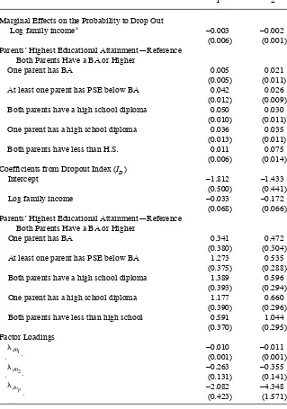
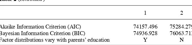
Table 2 reports the marginal effects and coeffi cients describing the relationship be-tween parental education and family income estimated in two different factor models. The fi rst column contains results from our extended system estimator that allows the distributions of the three factors to differ by parental education level. Note that this specifi cation nests the more standard model, where the distributions of the three fac-tors do not vary with parental education, as a special case. For comparison, in the second column we present results from the standard model. Using both the Akaike Information Criterion (AIC) and Bayesian Information Criterion (BIC) measures, the extended model represents a better fi t of the data.
In both columns of Table 2, the impact of family income is essentially zero: notably smaller than the already small impacts in Belley, Frenette, and Lochner (2008). The gradient in the marginal effects of parental education estimated in the fl exible factor model, and shown in Column 1, is fl atter than the reduced form and the standard factor model estimates. Examining the coeffi cients on the parental education variables in the second panel of Column 1 suggests that the effects on dropping out for the four lowest parental education categories are not signifi cantly different from each other. We focus on the gradient between families where both parents have a BA and families where both parents are high school dropouts because that is the steepest gradient in the raw data.
Table 2
Parental Education and Family Income Coeffi cients and Marginal Effects from Factor Models
1 2
Marginal Effects on the Probability to Drop Out
Log family incomea –0.003 –0.002
(0.006) (0.001)
Parents’ Highest Educational Attainment—Reference Both Parents Have a BA or Higher
One parent has BA 0.005 0.021
(0.005) (0.011)
At least one parent has PSE below BA 0.042 0.026
(0.012) (0.009)
Both parents have a high school diploma 0.050 0.030
(0.010) (0.011)
One parent has a high school diploma 0.036 0.035
(0.013) (0.011)
Both parents have less than H.S. 0.011 0.075
(0.006) (0.014)
Coeffi cients from Dropout Index (ID)
Intercept –1.812 –1.433
(0.500) (0.441)
Log family income –0.033 –0.172
(0.068) (0.066)
Parents’ Highest Educational Attainment—Reference Both Parents Have a BA or Higher
One parent has BA 0.341 0.472
(0.380) (0.304)
At least one parent has PSE below BA 1.273 0.535
(0.375) (0.288)
Both parents have a high school diploma 1.389 0.596
(0.393) (0.294)
One parent has a high school diploma 1.177 0.660
(0.390) (0.296)
Both parents have less than high school 0.591 1.044
(0.370) (0.295)
Factor Loadings d
1 –0.010 –0.011
(0.001) (0.001)
d
2 –0.263 –0.355
(0.131) (0.141)
d
p –2.082 –4.348
(0.423) (1.571)
possible unmeasured factors, the pattern implies that we really are capturing parental valuation of education rather than getting another measure of child abilities.
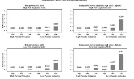
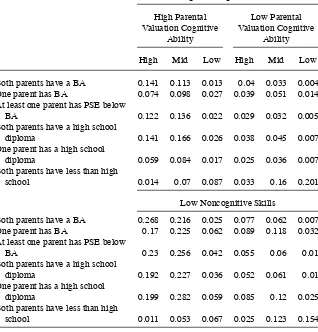
To further explore the effect of parents’ education and the direct impact of the fac-tors on dropping out, Figure 3 presents fi tted probabilities conditional on each pos-sible combination of the unobserved characteristics, based on the estimates from our extended factor model. Predicted probabilities for two BA families and two dropout families are shown in the fi rst and second columns, respectively. Probabilities for all other parental education categories are available from the authors. The fi tted values are the predicted probability for each individual evaluated at each possible combination of the mass- points in the factor distributions. Because there are three points of support in the cognitive ability distribution and two points in each of the noncognitive and pa-rental valuation distributions, this yields 12 fi tted probabilities for each individual. To estimate the probability for each parental education category, we take the simple aver-age of the fi tted probabilities across teenagers whose parents fall within the particular education category. The top panel of Figure 3 shows the fi tted dropout probabilities evaluated at high noncognitive ability and the bottom panel shows the same for low noncognitive ability.
With few exceptions, high- cognitive ability teenagers do not drop out regardless of their parent’s education or the values of the other factors. For teenagers with low noncognitive skills whose parents are high school dropouts and place low value on education, moving from high to low cognitive ability increases the probability of drop-ping out from 0.019 to 0.40. Parental valuation effects are nearly as large for teenagers with medium or low cognitive abilities. A teenager with low cognitive and noncogni-tive abilities whose parents place a high value on education has a 0.045 probability of dropping out, which means the impact of parents’ valuations for a low- ability boy is 0.36. Moreover, a student whose parents place a high value on education has essen-tially a zero probability of dropping out unless he has both low cognitive and noncog-nitive abilities, and even then his dropout probability is not statistically different from Table 2(continued)
1 2
Akaike Information Criterion (AIC) 74157.496 75284.279
Bayesian Information Criterion (BIC) 74936.928 76063.711
Factor distributions vary with parents’ education Y N
Source: Youth in Transition Survey, Cycle 3 (Cohort A)
Notes: Marginal effects are evaluated at the mean characteristics of a youth whose parents both have a high school diploma. Standard errors, clustered by high school, are reported in pararenthesis. Estimates are weighted to account for nonresponse to the parents’ survey and longitudinal attrition. Column 1 estimated from a model where the probability weights vary across parental education categories. Column 2 estimated from a model where the probability weights are the same in each parental education category. The model in Column 1 includes controls for province, the number of household moves, age in months, number of siblings, family structure and local youth unemployment rate. The model in Column 2 includes all these controls plus a control for Aboriginal status, immigrant status and living in a rural area. Cognitive skills are θ1, noncognitive skills are θ2, parental valuations are νp.
T
he
J
ourna
l of H
um
an Re
sourc
es
Table 3
Selected Estimated Parameters from Measurement Equations in Factor Model
1 2 1 2
Reading Scores (PISA)
Intercept 524.162 510.918 Variance ln(u
1
2) 3.968 4.151
(10.000) (5.322) (0.044) (0.026)
Parent’s Aspirations (Parpref)
Intercept 0.412 0.166 p
1 0.008 0.012
(0.161) (0.101) (0.000) (0.001)
p
2 0.103 –0.139 pp 1.097 2.482
(0.058) (0.144) (0.228) (0.858)
Not Wanting to Just Get By (getby)
Intercept –3.495 –3.156 c
p 2.853 11.898
(0.372) (0.281) (0.536) (3.937)
Grades (grd)
Intercept 67.390 59.288 g
1 0.091 0.115
(1.776) (1.190) (0.004) (0.005)
g
2 8.049 13.841 gp 11.646 39.364
(0.567) (1.949) (2.013) (12.121)
Variance ln(u
4
2) 1.857 1.464