ANUGA software for numerical simulations of shallow water flows.

ISSN

:

2O88-7O51

JOURNAL

OF

COMPUTER

SCIENCE

AND

INFORMATION

Volume 5, Issue 1, February 2012

Director:

T.

Basaruddin,

Universitas

lndonesia, Indonesia

Chief

Editor:

Wisnu

Jatmiko, Universitas Indonesia, Indonesia

Board

of

Editor:

Agus Buono,

Institut

Pertanian

Bogor,

lndonesia

Agts

Zainal

Arifin,

Institut Teknologi

Sepuluh

November,

Indonesia

Alwen

Tiu, Australian National University,

Australia

Aniati Murni,

Universitas

Indonesia, Indonesia

Belawati H. Widjaja, Universitas

lndonesia, lndonesia

Heru

Suhartanto,

Universitas

Indonesia, Indonesia

Hisar

Maruli

Manurung, Universitas

Indonesia, lndonesia

Ito

Wasito,

Universitas

Indonesia, Indonesia

Marimin,

Institut

Pertanian

Bogor,

lndonesia

M.

Rahmat

Widyanto, Universitas

Indonesia, Indonesia

Wishnu

Prasetya,

Universiteit Utrecht,

Belanda

Managing

Editor

:

Muhammad

H. Hilman, Universitas

Indonesia, Indonesia

Address:

Faculty of

Computer Science

Universitas

Indonesia

Kampus Baru

UI

Depok, I6424,Indonesia

T elp.

+62-21

-7 863

419,

F ax.

+62-21

-7 863 41 5

Email

:

jiki@cs.ui.ac.id

Website: http://j

iki.cs.ui.ac.id/

@enceandInformationisascientificjourna1incomputerscienceand

rnlbmration containing

the

scientific

literature

on

studies

of

pure

and applied research in

colnputer

science and

information

and

public

review of

the development

of theory,

method and

applied sciences related to the subject.

Journal

of

Computer

Science

and

Information is

published

by

the

Faculty

of

Computer S.-re

nce

UI.

Editors

invite

researchers,

practitioners,

and

students

to

write

scientific

;;1

slf

pille

rts

rn t-relds related

to

computer science and

information.

Journal

of Computer

Science

and

Information

is issued

2 (two) times

a year

in

February and

ISSN

:

2O88-7O51

JOURNAL

OF

COMPUTER

SCIENCE

AND

INFORMATION

Volume

5,

Issue

1,

February

2OL2

TABLE

OF

CONTENTS

1.

Anuga

Software

for Numerical Simulations

of

Shallow Water

Flows

Sudi

Mungkasi

and Stephen

Gwyn

Roberts

I

2.

Linkedlab:AData

Management

Platform for

Research Communities

Using

Linked DataApproach

Banz

Darari

and

Ruli

Manurung

g

3.

The Construction

of

Indonesian-English Cross Language Plagiarism

Detection

System

Using Fingerprint

Technique

Zal<ty

Firdaus

Atfikri

and

Ayu

Purwarianti...

...

16

4.

Local Btnarization

for

Document Images Captured

by

Cameras

with

Decision

Tree

Naser Jawas,

Randy

Cahya

Wihandika,

and

Agus

ZainalAnfin...

...

24

5.

Tendency

of

Players is

Trial

and

Error:

Case Study

of Cognitive Classification

in The

Cognitive

Skill

Games

Moh. Aries

Syufagi,

Mauridhi

Hery Purnomo,

and

Mochamad

Hariadi...

3l

6.

Model

Selection

of

Ensemble Forecasting

Using Weighted

Similarity of

Time

Series

Agus

Widodo

and

Indra

Budi...

...40

7.

Operating System

for

Wireless Sensor

Networks

And

An

Experiment of

Porting

ContikiOS to

MSP430

Microcontroller

Thang

Vu

Chien,

Hung

Nguyen Chan, and

Thanh

Nguyen

Huu

...

50

JgS[

llll

louRNAr

oF

coMpurER

scrENCE

AND

rNFoRMArroN

1.

ANUGA SOFTWARE FOR NUMERICAL SIMULATIONS OF SHALLOWWATER FLOWS

Sudi Mungkasil,2and Stephen Gwyn Robertsl

rMathematical _Sciences

Institute, Australian National University, Canberra, ACT 0200, Australia 2Department _{of Mathematics,}

Sanata Dharma University, Mrican Tromol Pos 29, yogyakarta 55002, Indonesia

E-mail: sudi.rnungkasi@anu.edu.au

Abstract

Shallow water llows are governed by the shallow water wave equations, also known as the Saint-Venant system. This paper presents a finite volume method used to solve the two-dimensional shallow water wave equations and how the finite volume melhod is implemented in ANUGA softw,are. This finite volume method is the numerical method underlying

thi

sofnvare. ANUGA is open source

software developed by Australian National University (ANU) and Ceoscience Australia

ice). rni,

software uses the finite volume method with triangular domain discretisation fbr the computation. Four test cases are considered in order to evaluate the performance ofthe software.'Overall. ANUGA is a robust sollware to simulate _{two-dimensional shallow water flows.}

Keyw'ords:.frite vohune methods, shallov, w'ater.flov,s, AN(\GA software, triangulctr grids, shollow water waNe equations

Abstrak

Arus air dangkal diatur dalam persamaan gelon-rbang air dangkal, dikenal sebagai sistem Saint-Venant. Penelitian

ini

menyajikan metode

finite

volume yang digunakan untut menyelesaikan persamaan gelombang

air

dangkal

dua

dimensi

dan

bagaimana metode

.finite

t,olume

diimplementasikan dalam perangkat lunak ANUGA. Metode _Jinite volurne adalah metode nurnerik yang mendasari perangkat lunak ANUGA. ANUGA sendiri adalah perangkat l|lnak open source yang dikembangkan oleh Australian National University (ANU) dan Geoscience Australia _iGe;. perangkai

lunak ini menggunakan metode _Jinite volume dengan diskritisasi domain segitiga dalam prises

komputasi. Empat

uji

kasus digr-urakan untuk mengevaluasi kinerja perangkat lunak. Secara

keseluruhan, ANUGA adalah perangkat lunak yang _{robust untuk mensimulasikan aua drmensi aliran} arus air dangkal.

Kata Kunci:.f nile vohrme methods, shallov'.,r,ater.flows, ,INUGA soJtwttre, triangilar gritls, shallow ytater t|ave equotiorls

Introduction

Since the nineteenth century

the

shallow water wave equations have emerged as important

mathematical models

to

describe water flows. Some

of

its

developments and applications are

given byRoberts et al.

Il-5],

_{and Stoker [6].}

In

1892, Riter

[7]

studied dam

break

modelling analtltically. This old work has had a

big

impact as

the

dam break problem

is

now becoming

a

standard benchmark

to

test

the perfonnance of numerical methods. Even though

this

problem

is

originally

modelled

for

one-dimensional shallow water wave equations,

it

can

also

be

treated as

a

two-dimensional problem,

which we present

in

this paper as a planar dam break problem.

In

addition,

it

can also

be

extended to a circular two-dimensional problem.

Oscillation

of

water on a paraboloid canal developed

by

Thacker

[8] is

another benchmark

problem,

which

is

interesting,

and

usually considered

by

shallow water researchers

to

test their numerical methods. This problem involves a wetting and drying process, a process that is

well-known

to

be very diffrcult

to

resolve _19-131. Yoonand Cho _[14] used this type

of

problem to

test their numerical method.

To complete testing a numerical method, a steady

flow

problem must also be performed in addition

to

unsteady

flow

test problems.

In

this This paper is the extended version from paper titled ,'A

finite volume method for shallow water flows on triangular

computational grids" that has been published in proceeding _of

2 _Journal of Computer Science and Information,Volume 5, Issue 7, February 2072

paper,

we

do perform

a

steady

flow involving

a

shock over a parabolic obstruction. This test case

is

usually used

iq

testing

a

one-dimensional shallow water solver.

One open-source free software developed to simulate two-dimensional shallow water

flows

is

ANUGA,

named

after

Australian

National

University

(ANU)

and

Geoscience Australia

(GA). This software uses a finite volume method as the underlying mathematical background. We

will

present this finite volume method and test the

performance

of

ANUGA using the

planar dam

break

problerrl

circular dam break

problern, oscillation on a paraboloid channel, and a steady

flow

over an obstruction. ANUGA uses triangular

domain discretisation for the computation. The remainder

of

this paper is organised as

follows.

In

Section

2,

we

present

the

shallow water wave equations governing water flows, the

finite

volume method and the

ANUGA

software. Section

3

contains

four

numerical

simulations

involving

unsteady

and

steady

flow

problems. Finally, Section

4

concludes the paper

with

some remarks.

2.

Methodology

Shallow

water

Wave

equations,the

one-dimensional shallow water wave equations can be written as

et*

f(Q)*=

s.

(1)

The

notations used

here are

described as

follows: q

=

lhuhlr

is

the

vector

of

conserved

quantities consisting

of

water

depth

h

and momentum

uh,

f

(q)

=

luhuzh +

g,hz

/2)r

is the

flux

function, s

=

[0 -

grh(z* +

r/)]r

is the source

vector

with

ry'

is

some defined friction terms,

x

represents the distance variable along the

flow,

t

represents the

time

variable,

z(x)

is

the

fxed

water bed,

h(x,t)

is the height of the water

at point

xand

at

time

t,

u(x,t)

denotes the velocity of the water

flow

at point

x

and attime

t,

and

g,

is a constant denoting the acceleration due

to

gravity.

In

addition, a new variable called the stage can be defined as

w(x,t)

=

z(x)

+

h(x,t)

which is the absolute water level.

More

general equations governing shallow

water

flows

are

the

two-dimensional shallow water wave equations

U5-20]

qt+f(q),* g(e)y=s

(2)

where q

=

lh

uh

uh)r

is the vector ofconserved

quantities consisting

of

water depth

h,

x'

momentum

uh,

and

y-momentumvh.Herc,u

and

u

are velocities

in the

x-

and y-dkection;

f

(q)

afi

g(q)

are

flux

functions

in

the

x-

and

y-direction given by

and

The source term including gravity and friction is

(3)

luhl

f

(q)

=lurn+ln,n

l

luvhl

s(q)=1",^{L.^,7

(5)

, =l-n,n1),*

r,.1]

l-s,n(2,

+

Sp)l

@)

where

z(x,y)

is

the

bed topography, and Sy

=

lS?-

+

S7^,

is

the bed friction

modelled using

{" lt

Manning's resistance law

^ ur;"lffi

;fx

=

-tW-(6)

and

w2",/;ry

rfr

=

-n+/z

Q)

in

which

4

is the Manning resistance coefftcient.

It

should be noted that the stage (absolute water

level)

w

is given by

w

:= z

*

h. In this paper, we focus on the two-dimensional shallow water wave equations.

Integrating equation

2

over

an

arbitrary

closed and connected spatial domain

O

having

boundary

f

and applyrng

the

Gauss divergence theorem to the flux terms, we get the integral form

where

F

=

VQ)

g@)lr

is the flux function,

n

=

[cos(g) sin(6)]r

is

the outward normal vector of the boundary, and

0

is the angle betweenn and thex-direction. Equation

8 is

called

the

integral

form

of

the two-dimensional shallow water wave equations.

*l,rdo+

f,

F'ndr =

I,'on

(8)

-Mungkasi, et al., Anuga Sofavare _for Numerical simulations of shallow water Flows 3

where

I

is the transformation matrix

[1

0

0r

r

=

l0

cos(d)

sin(e)

l.

[o

-

sin(o)

cos(g)l

Therefore, equation 8 can be rewritten as

*.;,A,Hritii=si

*L

,

do+

*

ruf

(rq)

try

=

!,

s

de

(11)

Finite

volume

method,a

finite

volume

method is based on subdividing the spatial domain

into

cells and keeping track

of

an approximation

to

the integral

of

the quantity over each

of

these

cells.

In

this paper,

we limit

our presentation for

triangular computational grids (cells).

After the

spatial domain

is

discretized, we have the equation constituting

the

furite volume

method over each triangular cell of the _{grids [16]}

The rotational

invariance

property

of

the

shallow water wave equations implies that

F

.n

:

T-'f

(Tq)

(9)

Here,

we

recall

the

algorithm

to

solve the two-dimensional shallow

water wave

equations

given

by

Guinot

[15].

In

the

semi-discrete

framework, four steps are considered as follows:

For

each interface

(i,

j),

transform

the

quantity

qi

and q1 in the global coordinate system

(x,y)

:r;rto

the quantity

Qi

and

47

in

the

local coordinate system system

(ft,i).

The water depth

h

is unchanged as

it

is a scalar variable, while the velocities

u

and

v

are transformed

into

0

atd

A.

Therefore,

the new

quantities

in

the

local

coordinate system axe

Q,

=

TQ, and

Qi

=

Tqi

(16)

whereq;

=

ln,1nu1r

1nv1rl ,

qj

=

lh1(hu)1 (hu)lare,

respectively, the quantities in

the global coordinate system. The matrices

T

and

T-7

are

(17)

(18)

Coi.rpute the

fiux

i

atthe inrerface (t,

j).

ht the local coordinate system, the problem is merely a one-dirnensional Riemann problern, as the

flux

vector

is parallel with

the rrormal vector

of

the interface. Therefr-rre,

the

equations

to

be

solved

are

Q,*

f(q)o=

s ( 1e)

with initial

condition given

by

Q; on one side

of

the interface (i,

j)

_{and 47} on the other side

of

the interface

(i,j). It

should be stressed that

at

this

step,

we

do not need

to

integrate equationlg for

the

quantity

_Q,but all we need is the value of the

flux

f.

Hence, applying either

the

exact

or approximate Riemann solvers to compute the

flux

i

atthe interface (1,7)

is

enough. Note that here the source term does not need to be transformed in

the

local

coordinate systern,

since

it

involves

scalar variables only.

Transform

the

flux

fback

coordinate system

(x,y),so

the

(10)

From

(15)

,[:

*,:?A

and

"=fi

:tr;;l']

(t2)

whereq;

is

the

vector

of

conserved quantities

averaged over

the lth

cell

s; is

the source temr

associated

with the

ith

cell,

Hi;

is the

outward

normal

flux of

material across the _ryth edge, and

l;;

is

the

length

of

the

ijth

edge. Here,

fhe

ijth

edge is the interface between the

lth

and

/th

cells.

The

flux

H;7 is evaluated using a numerical

flux

function

H(.,.;.)

such

that

for all

conservation

vectors q and normal vectors n

H(q,q;n) =

F .n.

Furthermore,

H _i1

=

H (qi(mi1), _{e 1}

(mt);

ni)

( 13)

(14)

where mi1 is the midpoint of the

ijth

edge

arrdnil

is the outward normal vector,

with

respect to the

Ith

cell,

on

the ryth

edge.

The function

q;

is obtained from the averaged values of quantities in

the lth and neighbouring cells.

Now

let

ni1= fnff)

"grlr.

equationl3and equationl4, we have

Hu =

flqi(mi)lnr+

O[71(mi)]nr.

to

the

global

4

lournal

of computer science and Information, volume 5, lssue 1, February 2072

midpoint

of

the

interface

(r,i)in

the

global

coordinate system is

Hij

ri'i

r;liGi;Q13i;3)

:

T;Li(TqoiiTilQl

sii s1). (20)

Here,

fis

the

flux

computed

with

a

Riemann

solver

for

the one-dimensional problem stated in Step 2.

Finally, solve equationl2 where

-lf(r)

=

t0,1,2\, as triangular grids are considered,

for

qi.

We

multiply

Hi1

with

l;;

in

order

to

get the

flux

over the interface

(i,l).

This is because the flux at

the midpoint of the interface

(i,i)

is

H;;,

and the

lengthof the interface

l;;.

In

this part, we briefly

describe

an

open-source

free

software

developed

using mathematical models described

in

the

previous

sections

called

ANUGA.Uppercased

word

'ANUGA'

refers

to

the

name

of

the

software,

whereas lowercased

word

'anuga' refers

to

the

name

of

ANUGA

module

in

programming. See

ANUGA

User

Manual for the

details

of

anuga

tl4l.

ANUGA is an

open source (free software)

developed

by

Australian National

University

(ANU)

and Geoscience Australia (GA) to be used for simulating shallow water flows, such as floods

and

tsunamis.

The

mathematical background

underlying

the

software

is

the

two-dimensional shallow water wave equations and

finite

volume method presented

in

Sections

2

and 3 above. The

interface

of this

software

is in Plthon

language,

but the mostly expensive computation parts, such as

flux

computation, are written in C language.

A

combination of these

two

languages provides two different advantages:

Plthon

has the

flexibility

in terms

of

software engineering,

while

C

gives a

very fast computation.

As has been described

in

the

ANUGA

User Manual

[16],

a simple simulation using

ANUGA

generally

has

five

steps

in

the

interface code. These five steps are importing necessary modules, setting-up

the

computational domain, setting-up

initial

conditions, setting-up boundary conditions,

and

evolving

the

system through time'

_.The necessary modules

to

be imported are anuga"and some standard

libraries

such

as numpy,

scipy,

pylab,

and

time. The

simplest creation

of

the

triangular

computational

domain

is in

the

rectangular-cross

framework,

which

returns

points,

vertices,

and

boundary

for

the computation.

The

initial

condition

includes the defrnition

of

the topography,

friction,

and stage. The boundary conditions can be chosen in several

ways depending on the needs: ret'lective boundary

is

for

solid reflective wall; transmissive boundary

is for

continuing

all

values

on

the

boundary;

Dirichlet

boundary

is

for

constant boundary values; and time boundary

is for

time dependent

boundary.A thorough description of

this

software

is available at http : I I arritga. anu. edu. au.

3.

Results and Analysis

This

section presents some computational experiments using the finite volume method with

ANUGA as

the

software used

to

perform the simulation.

For

simplicity

of

the

experiments,

frictionless topography is assumed. Four different

test

cases

are

considered:

a

planar dam

break

problem, circular

dam

break problem,

water

oscillation

on a

paraboloid channel, and steady

flow

over a parabolic obstruction.

The numerical settings are as

follows'

Even though

ANUGA

is capable to do the computations

with

unstructured triangular grids,

we

limit

our

presentation only to the structured triangular grids

-for

brevity

with

rectangular-cross as

the

basis.

The

spatial

reconstruction

and

temporal

discretisation

are both

second

order

with

edge

limiter.

A

reflective boundary

is

imposed. The numerical

flux

is due

to

Kurganov et al.

[21].

SI [image:7.602.315.510.432.478.2] [image:7.602.318.511.518.706.2]

units are

used

in

the

measurements

of

the quantities.

Figure 1. Initial condition for the planar dam break problem'

Figure 2. Water flows 0.5 second after the planar dam is

broken.

Figure 3. Water flows 1.0 second after the planar dam is

broken.

Consider

a flat

topography

without

friction

on

a

spatial domain given

by

{(x'v)l(x'v)

e

planar dam break problem

with

wet/dry interface

bewtween

the

dam, where

we have 10

meters

water depth on the left of the dam, but dry area on the right. The dam is at

{(0,y)ly e [-10,10]].

The simulation

is

then

done

to

predict

the

flow

of

water after

the

dam

is

removed.

Note that

this dam break problem is actually a one-dimensional dam-break problem,

but

here

we

treat

this

as a

two-dimensional problem.

Figure 4. Water flows 1.5 seconds after the planar dam is

broken.

Figure 5. Initial condition for the circular dam break problem.

Figure 6. Water flows 0.5 second after the circular dam is

broken.

Figure 7. Water flows 1.0 second after the circular dam is broken.

The domain setting is as follows. The spatial

domain is discretised

into

1-00

by

20 rectangular-crosses,

where each

rectangular

cross

has

4

uniform

triangles.

This

means

that we

have B.

Mungkasi, et al., Anuga Sofrware _for Numerical Simulations of Shallow Water Flows 5

103structured triangles as the discretisation of the spatial domain.

The water surface and topography are shown

in

figurel,

2, 3,

and4.

In

particular,

figure

I

shows

the initial

condition, that

is,

the

water

profile

at

timet

=

0.0 s.

After

the dam is broken,

the

profiles

at

time

f

=

0.5, 1.0, 1.5

s

are

illustrated

in

frgure

2,

figure

3,

and

figure 4

respectively.

At

1.5 seconds after dam break, the

water flows

to

the right

for a

distance almost 30

m.

This

agrees

with

the

analytical solution (30

m) for

the

one-dimensional

dam

break

problem.

Figure 8. Water flows 1.5 seconds after the circular dam is

broken.

Now

suppose

that we

have

a

circular dam break problem

with

wet/wet interface between the

dam. Consider a circular dam, where the point

of

origin is the centre, having 20 m as its radius. The

water depth inside the circular dam is 10 m, while outside

is

1

m.

The

spatial domain

of

interest

is{(x,y)l(x,y)

e

[-s0,s0] x

[-s0,s0]].

Similar

to the planar dam break problem, the simulation

of

this test case is then done

to

predict the

flow

of

water, after the dam is removed.

The domain setting is as follows. The spatial

domain is discretised into 100 by100 rectangular-crosses,

where each

rectangular

cross

has

4

uniform

triangles.

This

means

that

we

have4. L0astructured triangles as the discretisation of the spatial domain.

The water surface and topography are shown

in

figure

5, 6, 7,

and

8.

In

particular,

figure 5 shows

the initial

condition, that

is, the

water

profile at time

t

=

0.0 s. After the dam is broken,

the profiles at time

t

=

0.5, 1.0, 1.5 s are illustrated

in

figure 6, figure 7, and figure 8 respectively.

At

1.5 seconds after dam break, the water floods to

the

surrounding

area

approximately

25m

outwards.

This test case

is

adapted from the

work

of

Thacker

[8]

and

Yoon and

Chou

[4].

Suppose

that we

have

a

spatial

domain

given

by _{(x, y)l (x,

y)

E _[-4000,4000]

x

_{[-4000,4000]].}

We

define

some

parameters Do

=

1000,

I

6 Journal of Computer Science and Information, Volume 5, lssue 1, February 2012

.

Lo-Rt

A=

I:++Rt

2

(21)

(22)

(23)

steady

shock.

Suppose

that

we

have

a

spatial

domain

given

byt@,y)l(x,y)

€ _[0,1s]

x

[0,1s]].

We

consider

the

topography

as

horizontal bed except for a defined parabolic obstruction

z(x,y)

=

0.2

-0.05(x

-

70)'

(27)

for

8 <

x

<-72. We use Dirichlet boundaries

for

the left

and

right

boundaries.

The

left boundary

is

set

up

as water height 0.42,

[image:9.604.152.300.92.196.2] [image:9.604.322.517.347.723.2]

x-momentum 0.18, and y-momentum 0.0. The right boundary

is

set

up

as water height 0.33,

x-momentum 0.18, and y-x-momentum

0'0.

The

initial

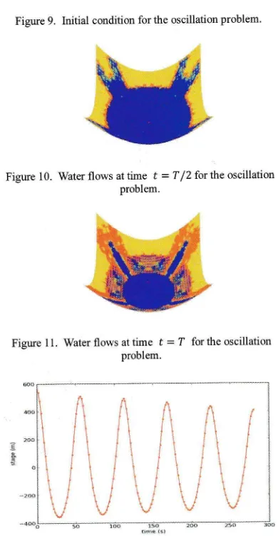
condition is just a quiet lake at rest with the stage level as 0.33.

Figure 9. Initial condition for the oscillation problem.

Figure 10. Water flows at time t ₌ T _/2 for the oscillation

problem.

Figure 11. Water flows at time t ₌

7

for the oscillation

problem.

Figure 12. The water surface corresponding to the origin until

t = 5T for the oscillation problem. 2tt

T-_

l-a

z(x,y)

-

-Do(r-i)

Af

I\I

ti

1t

\/

\l

\t

/i

/\

t\

tl

Itlt

Itlt

Itt!

I\/\

ItI\

.ltl

\

I

\1

LlV

A

Jl

I

t

ti

\l

ltt=-L{2g,Do

are the amplitude

of

oscillation at the origin, the

angular frequency, and the period

of

oscillation.

Furthermore, the topography is given by

(24)

and the

initial

water level (the

initial

wet region)

is

I ^lt-T

h(x,y) =

Do

[r

_

a.*frrl

-

1

-,(n-ffi#-')l

(2s)

where

,

=

r1r,

+1,

. (26)

The domain setting is as follows. The spatial domain

is

discretised

into 50 by 50

rectangular-crosses,

where each

rectangular

cross has

4

uniform triangles. This means that we have 104

structured triangles as

the

discretisation

of

the spatial domain.

The simulation

is

then done

to

perdict the

flow of

the water. According

to

Thacker

[8],

the flow

will

be a periodic oscillation. The simulation,

using

the

numerical

method

and

software

discussed in this paper, indeed shows this periodic

motion. The water profiles at

time t =

0, T

/2,

T

are

shown

in

figure9,

figure

10, and

figure

ll

respectively.

In

addition, the periodic motion

of

the water surface corresponding

to the origin

is

depicted

in

figure 12. From the numerical results,

we

see

a

minor

damping

of

the

oscillation. However, a perfect method or software should not

produce

this

damping. Although

it

may

be

impossible to have a perfect method, we take this

for

future research

for

the

ANUGA

software to

minimise

or

eliminate this

kind of

damping. We

also

see

from

the

numerical results

that

a

negligible

amount

of

water

is left

over

in

the supposed-dry area.

Steady

flow

over a parabolic obstruction,this

test case is for checking if ANUGA can produce a

Mungkasi, et al., Anuga Sofrware _for Numerical Simulations of Shallow Water Flows 7

The domain setting is as follows. The spatial

domain

is

discretised

into

720

by

120 rectangular-crosses, where each rectangular cross has

4

uniform triangles. This means that we have

57,600structured triangles as the discretisation

of

the spatial domain.

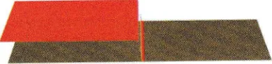
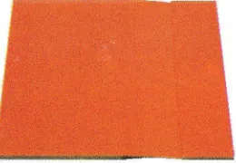
The summary

of

the simualtion results is as

follows. Figures 13 and 14 show the water surface

at initial condition and at time

t

=

25. After water

is flowing for 25

seconds

from left

boundary to the

right,

a steady shock occurs on the parabolic obstruction. This agrees with the simulation using

purely one-dimensional model using equationl in

our previous _{work [22].}

(It

is unfortunate that due [image:10.592.142.233.325.389.2]

to

the

small water height,

the

shock and

the

bottom topography

are

not

clearly

shownin

figure

14.

However, these

can

be

clearly

seen [image:10.592.125.255.427.517.2]

using ANUGA Viewer as pafts of the picture can be magnified.).

Figure 13. Steady flow over a parabolic obstruction at t = 0.

Figure 14. Steady flow over a parabolic obstruction at t = 25.

4.

Conclusion

We have presented some mathematical (both

analltical

and numerical) background underlying the

ANUGA

software.

ANUGA

was tested using

four

numerical simulations.

We infer from

the

simulation results that

ANUGA

can solve nicely

the wetting problem.

For

the drying

problenr,

some

very

small amount

of

water,

which

is negligible, may be

left

over on the supposed-dry area. Regardless of what we have investigated, we

need

to

note

that

different

parameters or

numerical settings generally

lead

to

different results. We also note that

ANUGA

can simulate

both steady and unsteady state problems.

Acknowledgment

The

work

of

Sudi Mungkasi was supported

byANU

PhD andANU Tuition Scholarships.

References

t1l

S.

Mungkasi

&S.G.

Roberts,

"A

finite volume method

for

shallow water

flows

on

triangular

computationalgrids"

In

Proceedings of International Conference on

Advanced Computer

Science

and

Information System (ICACSIS) 2011, pp. 79-84,2011.

[2]

S.G. Roberts

&P.

Wilson,

"A

well

balanced scheme for the shallow water wave equations

in

open

channels

with

(discontinuous)

varying

width

and

bed," On

ANZIAM

Journal,

vol.

52(CTAC20I0),

pp.

C967-c987,201r.

[3]

J.D. Jakeman,

N.

Bartzis, O.M. Nielsen,& S.

Roberts,"Inundation

modelling

of

the december

2004

ndian

ocean

tsunami" In

Proceedings

of MODSIM)7, pp.

1667-1673,

2007.

[4]

S. Mungkasi

&

S.G. Roberts,

"On the

best quantity reconstructions

for a well

balanced

finite

volume method used

to

solve

the

shallow water wave equations

with

a wet/dry

interface"

On

ANZIAM Journal,

vol.

5 1(EMAC2009), pp. C48-C65, 2010.

S.G. Roberts,

O.M. Nielsen,& J.

Jakemarl

"Simulation

of

tsunami

and flash

floods,"

Modeling Simulation and Optimization

of

Complex Processes"

In

Proceedings

of

the

International

Conference

on

High

Performance Scientific Computing,

pp.

489-498,2008.

J.J. Stoker, Water Waves: The Mathematical

Theory

with

Application,

Interscience Publishers, New

York,

1957.

A. Ritter, "Die

fortpflanzung

der

wasserwellen,"

Zeitsckift

des

Vereines

Deutscher Ingenieure,

vol.

36(33),

pp.

947-954, t892.

W.C. Thacker, "Some exact solutions

to

the nonlinear shallow water equations," Journal

of Fluid

Mechanics,

vol.

107,

pp.

499-508,

198 1.

K.

Ganeshamoorthy,

D.N.

Ranasinghe,

K.P.M.K. Silva,&R. Wait,

'?erformance

of

shallow

water

equations

model

on

the computational

grid

with

overlay

memory architectures"

In

Proceedings

of

the Second

Intentational

Conference

on Industrial

and

tsl

t6l

U]

t8l

8 _{lexrrnal af {amprufer} ..S'cfer ee and Infarmation, ValLtma

.i

Issue 1, Fehrtiary 2 A 1.2

Informiirion S\,,stems, pp. 415-120, 2007.

[10]

S.

Guangcar,

\i/.

Wenii,&Y.L.

I-.iu,

'Nurnerical sci:enie

for

simulation

of

2;il

flood

waves"

ln

Frocee;"iirtg.s

o/

the

In terncttional Conference

on

L'ontpulctri o;tal

and

Infbrmation

Science,s,

pp.

E46 849,

2010.

[1i i].D.

Jakeman, 0.1\{. }lielsen,

K.V.

Pr"rtten, R.

N{leL:zko,D.

i}urbidge,&t'i.

}lors1:.;.rol,

"T'orvarcls spatiaUy

distributed

quantitative

assessmeot

of

tsunami inr=indation mor1eis'"

International fi/orkshop

an

lvlocleling the

Acean

(IIl'M()):

D1'namics, Syntheses ,tn:l Prediction,."ol. 60(5), pp. 1115-l138, 20i0.

[12]C. Lu, Y.

Chen,&G.

i.i,

"rAreighted essential

non-oscillatory schemes

for

simulations

of

shallow u,ater

equations

rvith

transport

of

pollutant

on

unstructured

meshe

s"

In

Proceedittg,s

of

the

Fourth

International Con-fbrence

on

Informcttion

and

Computing,

pp.

174

l11,2}ll.

[3]S.

N'Iungkasi

&S.G.

Roberts,

"Apprcximations

of

the

can'ier-sreens'ilan

periociic sohrtion

to

the shallow wafer $,ave eqr-rations

for

florvs

on

a

slopirig

bcach,"

tr n te rnati o na| ..\ourna! _.{or Numeric

aI

lll{eIhods

in

Ftuids.20lt.

[14] S.B. Yoon

&i.]{.

eho, 'Numericai simulation

of

coastal inundation

over

disconlinuous

topography,"

ll'ater

Enginetring

ReseurLh,

'..'o1. 2(2), pp. 75-87, 2001.

[5]

V.

Cuitrot,

Wave

propagation

in

.fluid,s:

models and ntnnerical technique.r. ISTE I-td (and John

Wiley

&

Sons, Inc). London (and Iloboken), 2008.

Iii]l

S.

Roberls,O. Nielsen,D.

Gray,&J.

Sexton,ll/UGl

Llser ilfarurul,

Geoscience

Australia,2010.

Ii

] j

W.

Tan,

Shallow v)ater

h),drodt'namic.s,

Elsevier Science Publisirers,

Amsterdani,

1992.

[181 C. Zoppc'rr &S. Roberts, Shallow water wa!'e

equations,

Australian National

University, book ur pruparation.

[19]C.

Zoppctu

&S.

Roberts,

"Catastrophic collapse

of

water supply reservoirs

in

urban

areas,"

,lournal oJ

H-vdraulic Engineering,

Arnerican Society

of

Civil

Engineers, vol.

125(7), pp. 686-695, 1999.

i20lC.

Zoppou

&S.

Roberts,

"Explicit

schemes

fbr

dam-break simulations,"

Journal

oj' Hydraulic Engineeriitg,

vol

129(1),

pp.

11

34.2003.

i21]A.

Kurganov,

S.

Noeile,&

G.

Petrova, "Semidiscrete

centrai-upwind

schemes for

hlperbolic

conservation lau.s and

harnilton-jacobi ecpati ons,

"

SI A A.[ .Iott r nal o/ Scient ifi c

Compitring. r,o1. 23(3), pp.

707

I 40, 2001.

l22lS.

Mungkasi

&

S.G.

Roberls, 'Numerical

entropy production

for

shallow water flows,"

ANZIAItI Journal,

vol.

52(CTAC20i0),

pp.