Wiley Global Positioning Technologies And Performance Mar 2008 ISBN 0471793760 pdf

(1)

(2)

Global Positioning

TECHNOLOGIES AND

PERFORMANCE

(3)

(4)

(5)

(6)

Global Positioning

TECHNOLOGIES AND

PERFORMANCE

(7)

Published by John Wiley & Sons, Inc., Hoboken, New Jersey Published simultaneously in Canada

No part of this publication may be reproduced, stored in a retrieval system, or transmitted in any form or by any means, electronic, mechanical, photocopying, recording, scanning, or otherwise, except as permitted under Sections 107 or 108 of the 1976 United States Copyright Act, without either the prior written permission of the Publisher, or authorization through payment of the appropriate per-copy fee to the Copyright Clearance Center, Inc., 222 Rosewood Drive, Danvers, MA 01923, 978-750-8400, fax 978-646-8600, or on the web at www.copyright.com. Requests to the Publisher for permission should be addressed to the Permissions Department, John Wiley & Sons, Inc., 111 River Street, Hoboken, NJ 07030, (201) 74-6011, fax (201) 748-6008.

Limit of Liability/Disclaimer of Warranty: While the publisher and author have used their best efforts in preparing this book, they make no representations or warranties with respect to the accuracy or completeness of the contents of this book and specifically disclaim any implied warranties of merchantability or fitness for a particular purpose. No warranty may be created or extended by sales representatives or written sales materials. The advice and strategies contained herein may not be suitable for your situation. You should consult with a professional where appropriate. Neither the publisher nor author shall be liable for any loss of profit or any other commercial damages, including but not limited to special, incidental, consequential, or other damages.

For general information on our other products and services or for technical support, please

contact our Customer Care Department within the U.S. at 877-762-2974, outside the United States at 317-572-3993 or fax 317-572-4002.

Wiley also publishes it books in variety of electronic formats. Some content that appears in print, however, may not be available in electronic format.

Library of Congress Cataloging-in-Publication Data:

Samama, Nel,

1963-Global positioning : technologies and performance/Nel Samama p. cm.

Includes bibliographical references. ISBN 978-0-471-79376-2 (cloth) 1. Global Positioning System I. Title.

G109.5.S26 2008

623.890_3—dc22 _2007029066

Printed in the United States of America

(8)

FOREWORD

Positioning is a function that has always been of major importance in sustaining human activities, whether to explore new lands, improve conditions, or to conduct offensive or defensive warfare. In the past six decades, thanks to the arrival of elec-tronic and related technologies, positioning methods have made a quantum leap and can be applied with sufﬁciently low cost and low power miniature devices to be acces-sible to individuals. A leap in these technologies occurred with the introduction of the satellite-based Global Positioning System (GPS) in the 1980s. Superior availability, accuracy, and reliability performances outdoors resulted in a rapid and revolutionary adoption of the system worldwide. The development and successful commercializa-tion of GPS methods for indoor applicacommercializa-tions in the late 1990s is currently resulting in scores of applications and mass-market adaptation. Meanwhile, the introduction of other satellite-based systems has resulted in the use of a more generic label, namely Global Navigation Satellite Systems (GNSS) for a technology that is increas-ingly considered a public utility.

The author, Nel Samama, has done a wonderful job in compiling this

introduc-tory book onGlobal Positioningalong the above timeline. Although the focus is on

GNSS, as it should be, other earlier and current methods are clearly described in context. A full understanding of GNSS principles can be a frustrating experience for readers that are not familiar with the required fundamentals of celestial mechanics, signal processing, positioning algorithms, geometry of positioning, and estimation. These topics are well treated in the book and are supplemented by an introduction to modern receiver operation, indoor signal reception, and GNSS augmentation. Examples of applications, described in a separate chapter, illustrate well the utilization diversity of GNSS. The book concludes with an entertaining crystal ball gazing into the future. . .

Global Positioningkeeps the mathematical and physical baggage to a minimum in order to maximize accessibility and readability by an increasingly large segment of developers and users who want to acquire a rapid overview of GNSS. The book ﬁts nicely between existing introductory texts for non-technical readers and the more highly technical textbooks for the initiated engineers and will be of value for numer-ous college courses and industrial use.

PROFESSORGE´RARDLACHAPELLE

CRC/iCORE Chair in Wireless Location Department of Geomatics Engineering University of Calgary

(17)

(18)

PREFACE

This preface gives some ideas about the way this book has been written: the goals, the philosophy, and how it is organized. Within the “Survival Guide” series, it is intended to provide an overview of geographical positioning tech-niques and systems, with an emphasis on radio-based approaches.

The idea of this book is to give a summary of the past, the present, and the short-term progress of positioning techniques. In addition, the goal is to make it simple to under-stand the main trends and reasons for current developments. With the advent of the European constellation of navigation satellites, Galileo, the planned developments of GPS and GLONASS, and the potential arrival of the Chinese constellation, COMPASS, the positioning domain is experiencing a real transformation. It is likely that positioning will enter everyone’s lives, transforming then on a wide scale. An understanding of the fundamental principles, realizations, and future improvements will help estimate the real limitations of the systems.

An important part of the book is thus devoted to Global Navigation Satellite Systems (GNSS) — six chapters almost exclusively deal with matters relating to them. The history of navigation, from both the historical and the technical points of view, will assist in assessing the main advantages and disadvantages of the various possible solutions for positioning. Also of prime importance, two chapters are devoted to indoor positioning, which will provide an overview of the approaches currently under development.

The footnotes are designed to provide additional hints or comments to the reader. There is no absolute need to read them at ﬁrst sight, thus allowing for smoother reading. These notes are often based on personal comments and should be considered accordingly. Although positioning is the main subject, the approaches described are often also applicable to velocity or time determination, which are as important as location in numerous practical cases. Furthermore, the term positioning is used instead of localization because the raw piece of information is in fact positioning, and is the data this book intends to deal with. Localization usually describes the use of positioning for applications: it is a higher level concept.

The book is organized in six parts. The ﬁrst part includes Chapters 1 and 2 and gives a brief history of navigation from both the historical (Chapter 1) and technical (Chapter 2) points of view.

(19)

main techniques of positioning, including, for instance, Wireless Local Area Networks or mobile network approaches.

Chapters 5, 6, and 7 form the third part and give details of GPS, GLONASS, and Galileo. In order to allow a direct comparison, each chapter deals with the three con-stellations. Chapter 5 sets out a description of the above systems, Chapter 6 gives detail of the various satellite signals, and Chapter 7 deals with the acquisition and tracking of these signals.

Chapter 8 constitutes the fourth part and shows how to calculate a position once the measurements are available. The methods of calculation given in this chapter, although related to GNSS, are applicable to any positioning system.

Indoor positioning, as a fundamental current challenge in navigation systems, is dealt with in the ﬁfth part, and includes Chapters 9 and 10. Chapter 9 describes some non-GNSS-based techniques, while Chapter 10 is devoted to those using satellite signals, in one way or another. The ﬁrst part of Chapter 9 is a global introduction to the “indoor problem.” Note also that summary tables are provided at the end of Chapter 10, including all the indoor techniques described.

Applications, either current or future, constitute the last and sixth part of the book. Chapter 11 is a description of the main current applications and devices. Chapter 12, on the other hand, intends to analyze how everyone’s lives are likely to be modiﬁed in the coming years, with the wide availability of positioning for both people and goods.

Finally, exercises are designed to strengthen the understanding of some speciﬁc aspects of the chapters, but also to go one step further. To do this, further reading may sometimes be required. Many exercises are not calculation ones but rather oriented towards the analysis of the chapter contents.

(20)

ACKNOWLEDGMENTS

I now understand the reason why all writers thank their families and friends for their patience and abnegation: all these books and documents open on the table, all this time spent in front of the computer, all this energy spent on this piece of paper, these so frequent moments thinking of the best ﬁgures that could be used to show a particular aspect, and so on. May all of the people concerned have my real recog-nition for their continuous efforts.

More speciﬁcally, I would like to thank the people who agreed to read the early versions of the book. Their comments and suggestions have really improved the ﬁnal version in its legibility and pertinence. Thanks to Anca Fluerasu, Muriel Muller, Serge Bourasseau, Nabil Jardak, Marc Jeannot, Je´roˆme Legenne, Michel Nahon, and Per-Ludwig Normark.

Special thanks and much gratitude to Gerard Lachapelle who, in addition, agreed to write the foreword of this book and to Emmanuel Desurvire who answered my basic questions about writing such a book. Also a great thank you to Gu¨nther Abwerzger, Jean-Pierre Barboux, and Alexandre Vervisch-Picois for the very inter-esting comments they provided.

This book also would not have been possible without the constant understanding of the people of the Navigation Group of the Electronics and Physics Department of the Institut National des Te´lećommunications (INT), France. They have very often been obliged to carry on their activities alone. I would also like to thank former col-leagues, Marc François and Julien Caratori, who helped me, a few years ago, start the positioning-related activities at INT. Also important are all the students who have enriched our reflections with their work and valuable exchanges — thanks also to all of you.

Last but not least, another special thank you to Dick Taylor, who made many cor-rections to the English of the book — he is certainly the only person who will ever read the book twice!

(21)

(22)

CHAPTER

1

A Brief History of

Navigation and Positioning

In this chapter, we look back at the evolution of geographical positioning, from astronomical navigation of ancient days to today’s satellite systems. Major dates are given together with a description of the fundamental tech-niques. These techniques are essentially still used today. The development phases of modern satellite positioning systems are also provided.

As soon as human beings decided to explore new territories, they needed to be able to locate either themselves or their destination. At first, only terrestrial displacements were of concern, and the issue was to be able to come back home. The “come back” function was achieved by using specific “marks” in the landscape that had to be memorized. Quite quickly, because of the possibility of carrying very large loads by sea, maritime transportation became an interesting way of traveling. New needs arose regarding positioning because of the total absence of marks at sea. Thus, navigators had the choice of following the shore, where terrestrial marks were available, or of finding a technique for positioning with no visibility to the shore. This was the starting point of geographical positioning.

B

1.1 THE FIRST AGE OF NAVIGATION

The origins of navigation are as old as man himself. The oldest traces have been

found in Neolithic deposits and in Sumerian tombs, dating back to around 4000BC.

The story of navigation is strongly related to the history of instruments, although they did not have a rapid development until the invention of the maritime clock, thanks to John and James Harrison, in the eighteenth century. The ﬁrst reasons pushing people to “take to the sea” were probably related to a quest for discovery and the necessity of developing commercial activities. In the beginning, navigation was carried out

Global Positioning: Technologies and Performance. By Nel Samama Copyright#2008 John Wiley & Sons, Inc.

(23)

without instruments and was limited to “keeping the coast in view.” It is likely that numerous adventurers lost their lives by trying to approach what was “over the horizon.”

Hieroglyph inscriptions comprise the most ancient documents concerning ships and the art of navigation. Oars and a square sail mounted on a folding mast were the means of propulsion of the ﬁrst maritime boats, which followed on from ﬂuvial

embarkations (around 2500 BC). The steering was achieved with an oar used as a

rudder located at the back of the boat and maintained vertically. This conﬁguration

did not allow sailing in all wind conditions. Then came the Athenian trireme;

about 30 m long and 4 m wide, it was a military vessel with one or more square sails and two or three rows of rowers. The Roman galleys showed no great improve-ment over it. Compared to these military ships, commercial vessels had more rounded forms and only used sails for their displacement, oars being reserved for harbor maneuvers. Thus, navigation was only possible with restricted wind conditions, leading to the need for a good knowledge of the weather.

Thanks to this knowledge and in spite of the limited size of their boats and the rusticity of their navigation instruments, the Phoenicians, as early as the beginning

of the twelfth century BC, had moved all around the Mediterranean Sea. The

Carthaginians had even navigated as far as Great Britain and it seems they tried to sail around Africa with no success. Navigation was mainly achieved during the day, and the instruments used were the eyes of the navigators, in order to keep in sight of the coast, and a sounding line. When navigators had to travel by night, they used reference to the movements of the stars as had the Egyptians. Then, the Greek astronomer Hipparchus created the ﬁrst nautical ephemeris, and built the

ﬁrst known astrolabes (around the second century BC). It has to be noted that the

basics of modern navigation principles were already established then and only the technical aspects would be improved. For instance, current global navigation sat-ellite systems use reference stars (the satsat-ellites), together with ephemeris (to allow the receiver to calculate the actual location of the satellites), and highly accurate measure-ments. This latter requirement, together with the fact that current systems carry out distance measurements, are the main differences from ancient navigation.

The astronomical process was quite inaccurate and frequent terrestrial readjust-ments were required. Localization was even more complex because of the lack of mar-itime maps. The ancients rapidly drew up documents to describe coasts, landmarks, and moorings — this allowed coastal navigation. For the same purpose, and also for security reasons, lighthouses were built. The most famous is the one in the

harbor of Alexandria, built on the island of Pharos during the third century BC.

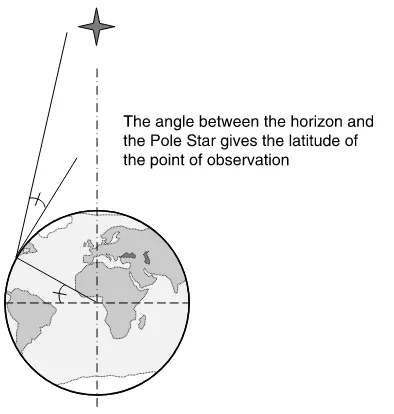
Unfortunately, astronomical positioning was only able to provide the latitude of a point, as can be understood from Fig. 1.1. The longitude problem would remain unresolved for centuries, as described in Section 1.2.

(24)

The sailor would put a speciﬁc knot between his teeth to deﬁne the actual “navigation parameters” for the current destination (latitude in this case). This was achieved by varying the distance the Kamal was from the teeth of the sailor, leading to a given angle.

Empirical knowledge of maritime currents has certainly been of great help for the navigators who planned incredible voyages, such as those undertaken by the people of the Polynesian islands. Northern Europeans also participated actively in the ﬁeld of

navigation, the story starting in the third centuryAD, with the ﬁrst attempts by the

Vikings to explore the northern Atlantic Ocean (the colonization of Iceland and

FIGURE 1.1 Determining latitude with the Pole Star.

FIGURE 1.2 The ﬁrst navigational instrument: the Kamal. (Source: Peter Iﬂand,Taking the Stars, Celestial Navigation from Argonauts to Astronauts.)

(25)

Greenland happened from the ninth century AD). The ﬁrst European discovery of

northern America, which they called Vinland, also happened in around 1000AD.

The medieval maritime world was separated into two areas: the Levant (the

Mediterranean area), where the Byzantines were leaders, and the Ponant, from

Portugal to the north, where Scandinavian maritime techniques were used. It was only at the end of the fourteenth century that the two types of techniques were joined, in par-ticular by using the stern-mounted rudder (appearing during the thirteenth century).

At around the same time, an instrument indicating absolute orientation appeared in the Mediterranean area, where the first reference to the magnetic needle for naviga-tion purposes was attributed to Alexander Neckam (around 1190). Since the discov-ery of the properties of a needle in the Earth’s magnetic field in the first or second century, it seems probable that the use of magnetism for navigation dates from

around the tenth centuryAD, in China. From then, the development of the compass

was continuous, starting with a pin attached to a wisp of straw ﬂoating on water, to the mounting of a dial to cancel out the vessel’s movements. Other important discov-eries include the determination of the difference between the magnetic north and the geographical north (ﬁfteenth century).

Although the compass was a fundamental discovery, it was far from the ﬁnal answer for ocean navigation. The main empirical characteristics of ancient navigation

remain: dead reckoning,1 which is based on the navigator’s expertise, imprecise

calculation of latitude by astral observations, and the deduction of the current location

using nautical ephemeris established in Spain during the thirteenth century AD

(Alphonsine tables).

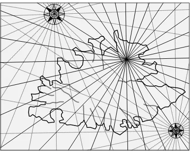
In any case, it would have been of no interest to establish a precise location without having similarly precise maritime maps, which was assuredly not the case. Following the maps of the world used during the eleventh century, the first maps showing the contours of the coasts associated with compass marks for orientation pur-poses appeared. These were the first portolan charts (Fig. 1.3), which show a set of crossing lines referenced to a compass rose (a specific representation of the compass). From the ideas of Ptolemy, the Arabians accomplished great cartographical

developments. For instance, Idrisi (1099 – 1165AD) drew a map that can be considered

as the synthesis of the Arabian knowledge of the twelfth century. It included details from Europe to India and China, and from Scandinavia to the Sahara.

Portolans were used to navigate from harbor to harbor. A network of directions referenced to the magnetic north allowed courses to be set. On such a map, infor-mation was available concerning the shore, but very little about the hinterland. The portolans are the main medieval contribution to cartography, and the precursors of modern maritime maps. An example of a sixteenth-century portolan of Corsica is given in Fig. 1.3.

One very important geographical area was the Indian Ocean. This zone was a meeting place for sailors from the Mediterranean, Arabia, Africa, India, and the Far East. The ancients well understood the advantage of the monsoon, and the ocean was a great opportunity for commercial exchanges. At the beginning, from the ﬁrst

centuryAD, the rhythm of the monsoon was well known, and Arabian and Chinese

(26)

(ninth century) sailors were already used to navigating in the ocean for commercial purposes. The adventures of Marco Polo (thirteenth century) and Ibn Battuta (fourteenth century) conﬁrm the persistence of such cultural and commercial exchange routes.

The Arabian navigation techniques used in the Indian Ocean were empirical approaches mainly based on the sidereal azimuth rose, which took advantage of the low latitude and navigation in clear skies. Such techniques took about two centu-ries to reach the Mediterranean region. The principle of such an azimuth rose is to divide up the horizon into 32 sectors using 15 stars scattered through the sky. It seems that Chinese navigators were a little ahead in terms of astronomical navigation, as well as magnetic tools. Their boats were also certainly more advanced concerning their sails, the axial rudder they used, and probably also a stern-mounted rudder. However, at the end of the Middle Ages, the Portuguese techniques of navigation had a deﬁnitive advantage.

B

1.2 THE AGE OF THE GREAT NAVIGATORS

From the middle of the fifteenth century there arose the need to find a route to the East for commercial activities with India, but which avoided the region of Persia. There were two possibilities: the first was to sail around the south coast of Africa and the second was to sail west, under the assumption that the Earth was a sphere. The Portuguese chose the first solution (led by Henry the Navigator) when Bartolomeu Dias reconnoitered the Cape of Good Hope in 1487. Following this first expedition, Vasco da Gama reached India around the aforementioned cape in 1498. The Spanish chose the second route, heading directly to the west across the Atlantic Ocean, and Christopher Columbus finally “discovered” America in 1492. The real west route to India was only discovered later when Magellan found the way through the Magellan strait to the south of South America in 1520. Figure 1.4 gives a global view of the most famous navigation routes. Note that in the Indian Ocean, Zheng He led many expeditions in the fifteenth century.

FIGURE 1.3 A sixteenth-century portolan of Corsica.

(27)

The navigation techniques, however, remained identical to those known and used at the end of the Middle Ages. The progress in navigation was mainly attributable to men’s skills and training. The Portuguese opened the Sagres School of navigation and the Spanish the Seville College, where the prestigious Amerigo Vespucci trained many famous sailors. Dead reckoning (with its associated accuracy), evaluation of currents, and the hourglass were the main methods and instruments used. A very important contribution due to Christopher Columbus was the discovery of magnetic declination and its variations.

The Portuguese and Spanish then decided to share the world, thanks to their mari-time superiority (Fig. 1.5). Despite the treaties of Tordesillas (1494) and Saragossa (1529), both nations had claims that could not be precisely checked because of the low accuracy of their positioning techniques, even on land. Remember that only the

FIGURE 1.4 The great navigators’ travels — ﬁfteenth century.

FIGURE 1.5 The great navigators’ travels — sixteenth century.

(28)

latitude of a location could be established, but not the longitude, as no technique was available. So territorial limits were defined through the help of significant land charac-teristics (river, mountains, and so on), but this was not a simple approach for countries located ten thousand miles away! Determining longitude on land was just about to find a satisfactory answer following Galileo’s work on Jupiter’s moons, but determining longitude at sea would remain impossible until the late eighteenth century.

The evaluation of latitude was based on the elevation measurement of a reference star over the horizon, which is a simple notion at sea. In the northern hemisphere, the

pole star2was established as the reference star at the very beginning of navigation, but

was not visible once in the southern hemisphere. The Portuguese, who had chosen to investigate the southern route around Africa, faced this problem quite early in the middle of the ﬁfteenth century. A new method was required, and it was found that the course of the Sun over the sky (and more precisely the elevation of the Sun

when passing through its apogee), together with astronomical tables (theregimentos),

allowed the evaluation of latitude worldwide.

To achieve the angle measurements required for both polar or Sun elevation, the instruments used were based simply on technical developments of the Kamal concept. The requirement was to make a double sighting: horizon and star. The ﬁrst instrument was a quadrant equipped with a sinker, allowing a direct reading of the latitude angle. Figure 1.6a shows the one attributed to Christopher Columbus.

FIGURE 1.6 A ﬁfteenth-century quadrant (a) and a seventeenth-century astrolabe (b). (Source: Peter Iﬂand,Taking the Stars, Celestial Navigation from Argonauts to Astronauts.)

2_{The Pole or North Star, Polaris, is at the very end of the Little Bear constellation. It is quite an important}

star, as it is almost exactly above the North Pole. Thus, its apparent movement is static, unlike the other stars that appear to move during the night due to the Earth’s rotation. The Pole Star was found to be a very good “reference light.”

The Greeks realized that Polaris was not exactly above the North Pole. We know that the reason for this is the slow movement of the Earth’s axis over thousands of years. It appears that 5000 years ago, a star called Thuban was nearest to the polar axis and, in 5000 years, Alderamin will be the one, and back to Polaris in 28,000 years.

(29)

The astrolabe (Fig. 1.6b), whose first use was to define the stars’ relative locations in the sky, was also adapted to navigation, allowing angle measurements. The moving part of the astrolabe, the alidade, is much better than the sinker for reading when the sea is rough. The main problem of both the quadrant and the astrolabe is that it is difficult to achieve the pointing of both the horizon and the star simultaneously. In addition, a direct sighting of the Sun is dazzling. Thus, another instrument was designed: the cross staff (Fig. 1.7). Its principle is to carry out a measurement of the length of a shadow cast by the Sun.

The use of reﬂection mirrors, attributed to Isaac Newton in 1699, allowed simul-taneous sighting of both the horizon and the star, using two mirrors (one of which was mobile). The sighting was then achieved in one go. The ﬁrst such instrument

was the octant, using a 458 graduated arc, soon followed by the sextant, using a

608graduation (Fig. 1.8). The compass was also updated by dividing it into 3608,

instead of 32 sectors, and adopting speciﬁc mountings in order to ease the plotting

of landmarks. Dead reckoning was also improved by the use of aloch, a new

instru-ment for measuring speed, simply composed of a hemp line graduated with knots that the navigator let out at sea for a ﬁxed period of time, deﬁned by the hourglass. Thus, he had an evaluation of the distance traveled during this time and consequently the speed of the boat.

Another important point was related to the evolution of maps. In the middle of the sixteenth century, Gerhard Mercator invented the projections that bear his name. This approach consisted of considering a representation in which the distance

between two parallels3increases with latitude. It was therefore possible to represent

the route that follows a constant heading by a straight line because of the conservation of angles. At the same time, the plotting of coasts was becoming better. Nevertheless, the problem of location accuracy remained, as longitude was still not measurable.

FIGURE 1.7 A Davis cross staff — sixteenth century. (Source: Peter Iﬂand, Taking the Stars, Celestial Navigation from Argonauts to Astronauts.)

3_{A parallel is a circle at the Earth’s surface being perpendicular to and centered on the North– South axis of}

the Earth. A parallel deﬁnes locations of equal latitude.

(30)

The conquest of new territories continued with the British, the French, and the Dutch during the eighteenth century. This was the time of expeditions in North and South America, and also in the Indian Ocean, trying to ﬁnd the best way to travel towards the East (Fig. 1.9). Cook’s famous expeditions to the Paciﬁc Ocean were also great chapters in this era of navigation.

It took almost three centuries for the longitude problem to be solved. During this period, signiﬁcant progress occurred in the development of instruments and maps, but nothing in determining longitude. As early as 1598, Philipp II of Spain offered a prize to whoever might ﬁnd the solution. In 1666, in France, Colbert founded the Acade´mie

FIGURE 1.8 An octant (a) and a sextant (b). (Source: Peter Iﬂand, Author ofTaking the Stars, Celestial Navigation from Argonauts to Astronauts.)

FIGURE 1.9 The great navigators’ travels — eighteenth century.

(31)

des Sciences and built the Observatory of Paris. One of his first goals was to find a method to determine longitude. King Charles II also founded the British Royal Observatory in Greenwich in 1675 to solve this problem of finding longitude at sea. Giovanni Domenica Cassini, professor of astronomy in Bologna, Italy, was the first director of the French academy, and in 1668 proposed a method of finding longi-tude based on observations of the moons of Jupiter. This work followed the obser-vations made by Galileo concerning these moons using an astronomical telescope. It had been known from the beginning of the sixteenth century that the time of the observation of a physical phenomenon could be linked to the location of the obser-vation; thus, knowing the local time where the observations were made compared to the time of the original observation (carried out at a reference location) could give the longitude. Cassini established this fact with Jupiter’s moons after having calculated very accurate ephemeris. Unfortunately, this approach requites the use of a telescope and is not practically applicable at sea.

In 1707, Admiral Sir Clowdisley Shovell was shipwrecked, with the loss of 2000 men, on the Scilly Islands, because he thought he was east of the islands when in fact he was west of them! This was too much for the British. On June 11, 1714, Sir Isaac Newton conﬁrmed that Cassini’s solution was not applicable at sea and that the avail-ability of a transportable time-keeper would be of great interest. It should be noted that

Gemma Frisius also mentioned this around 1550, but it was probably too early. . .On

July 8, 1714, Queen Anne offered, by Act of Parliament, a £20,000 prize4to whoever

could provide longitude to within half a degree. The solution had to be tested in real conditions during a return trip to India (or equivalent), and the accuracy, practicabil-ity, and usefulness had to be evaluated. Depending on the success of the correspond-ing results, a smaller part of the prize would be awarded.

The development of such a maritime time-keeper took decades to be achieved, but ﬁnally had an impact on far more than navigation. The history of Harrison’s clocks is quite interesting, and time is really the fundamental of modern satellite navigation capabilities. We have seen that Isaac Newton himself conﬁrmed that the availability of a transportable maritime clock would be the solution to the longitude problem. The realization of such a clock, however, was not so easy. The main reason is that the clock industry was fundamentally based on physical principles dependent on gravitation (the pendulum). This was acceptable for terrestrial needs, but of no help in keeping time when sailing. Thus, a new system had to be found.

The reason that time is of such importance is because of the Earth’s motion around its axis. As the Earth makes a complete rotation in 24 hours, this means that every hour corresponds to an eastward rotation of 158. Thus, let us suppose that one knows a reference conﬁguration of stars (or the position of the Sun or Moon) at a given time and for a given well-known location (e.g., Greenwich). If you stay at the same latitude, then you will be able to observe the same conﬁguration but at another time (later if you are eastward and earlier if westward); the difference in times directly gives the longitude, as long as the time of the reference location (Greenwich in the present example) has been kept. The longitude is simply obtained

by multiplying this difference by 158per hour, eastward or westward. The method is

(32)

very simple and the major difﬁculty is to “keep” the time of the reference place with a good enough accuracy, that is, with a drift less than a few seconds per day. Pendulums, although of good accuracy on land, were unable to provide this accuracy at sea, mainly because of the motions of the ship and changes in humidity and temperature.

John Harrison built four different clocks, leading to numerous innovative con-cepts. After almost 50 years of remarkable achievements, in August 1765 a panel of six experts gathered at Harrison’s house in London and examined the final “H4” watch. John and William (his son) finally received the first half of the longitude prize. The other half was finally awarded to them by Act of Parliament in June 1773. Certainly more important is the fact that John Harrison was finally recognized as being the man who solved the longitude problem.

One of the most famous demonstrations of Harrison’s clocks’ efﬁciency was pro-vided by James Cook during the second of his three famous voyages in the Paciﬁc Ocean. This second trip was dedicated to the exploration of Antarctica. In April

1772, he sailed south with two ships: theResolution and theAdventure. He spent

171 days sailing through the ice of the Antarctic and decided to sail back to the Paciﬁc islands. He returned to London harbor in June 1775, after more than 40,000 nautical miles. During this voyage, he was carrying K1, Kendall’s copy of Harrison’s H4. The daily rate of loss of K1 never exceeded eight seconds (corres-ponding to a distance of two nautical miles at the equator) during the entire voyage. This was the proof that longitude could be measured using a watch.

B

1.3 CARTOGRAPHY, LIGHTHOUSES AND

ASTRONOMICAL POSITIONING

It is quite obvious that before planning a route, knowing the current location is fundamental. The notion of route also means being able to “draw” the locations on a map. Thanks to Mercator, a graphical representation of the Earth was deﬁned that allowed angles to be preserved whilst projecting the sphere onto a plane (Fig. 1.10). This approach is essential, as it was thus possible to navigate following

FIGURE 1.10 The great Mercator’s projection.

(33)

a compass orientation, that is, a constant angle. The projection is carried out on a cylinder tangent to the Earth at the equator, and modiﬁes the projected values in such a way that a route crossing all the meridians with the same relative angle becomes a straight line in the projected plane. The shortest route from one point to another is then represented by a complex concave curve (because the constant-angle route is not the optimal one on a sphere).

Astronomical positioning is not very accurate, so sailors also used landmarks to keep track of their location. These terrestrial landmarks were sighted from the boat, allowing the plotting of a straight line passing through both the landmark’s location (which needs to be known, like the satellite locations in today’s satellite navigation systems) and the boat. The plotting of three such lines gave the theoretical location

of the boat.5 Of course, because of measurement errors and inaccuracies, this

would lead to the creation of a triangle, and the location was usually considered to be the center of the circle that could be drawn inside the triangle. Lighthouses are one of the most noticeable of the landmarks, but others include natural sights, buoys, and so on.

Astronomical positioning consisted of determining the location of the boat by measuring the heights of some given stars above the horizon (by using a sextant). The possible positions on Earth that exhibit the same observed height of a given star are located on a circle that is centered on the vertical line joining the star and the center of the Earth. The radius of this circle is dependent on the heights of the star above the horizon. Of course, the location of the reference star was required — this was obtained through ephemeris, which gave the exact locations of various stars according to the time. Calculating the position (described in Chapter 2) required two measurements to solve the set of two second-degree equations. To be rigorous, the two measurements should be carried out at the same time, otherwise complex recalculations are needed.

Positioning in ancient times was thus typically a discrete event. To be able to follow the location of the boat permanently, or at least to have an idea of its route, required so-called “dead reckoning.” The basic principle of this is to measure both the direction and the speed of the boat. In this way, the complete kinematics is deﬁned and the location can be evaluated with accuracy, as long as both the measure-ments and initial position are accurate. For a long time this was not the case, but the new radio electric techniques would bring about a revolution in positioning, as described in the following.

B

1.4 THE RADIO AGE

The desire to communicate over long distances was described long before the radio conduction phenomenon was discovered. The ﬁrst related facts using optical

means date from the fourth and ﬁfth centuriesBC, when ﬁres on the tops of mountains

were used to serve as “communication relays.” This approach was still being used by

(34)

the ﬁrst optical telegraphs in the seventeenth century. Of course, the main disadvantage of such a system lies in the fact that transmission is limited to the optical line of sight and requires good “air conditions,” that is, no fog. This problem led to the development of the electrical telegraph.

On November 24, 1890, Edouard Branly discovered the phenomenon of “radio conduction,” in which an electrical discharge (generated by a Hertz oscillator) had the effect of decreasing the resistance of his “tube.” It appeared that electrical propa-gation was possible without cables. Further work showed that adding a metallic rod to the generator improved the range of the transmission (that is, the detection was also possible further away from the generator). Alexander Popov was in fact just about to invent antennas. The transmission path grew from a few tens of meters to 80 m. In 1896, Popov succeeded in transmitting a message over 250 m (the message

being composed of two words, “Heinrich Hertz”).6

At the same time, Guglielmo Marconi, who was deeply inﬂuenced by the publi-cations of Faraday and the life of Benjamin Franklin, felt that it should be possible to establish a transmission over a few kilometers. After a lot of work, he transmitted the letter “S” coded in Morse (“. . .”) over 2400 m at the end of 1895. In September 1896, by using a kite as an antenna, Marconi achieved a 6 km, then 13 km radio path. In May 1897, a transmission of 15 km was demonstrated between two English islands (Steep Holm and Flat Holm), followed by similar performances in Italy in La Spezia harbor. Marconi founded, on July 20, 1897, the Wireless Telegraph and Signal Company. In March 1899, the ﬁrst trans-Channel message was sent between South Fireland (Great Britain) and Wimereux (France). The addressee was Edouard Branly. With antenna heights of 54 m, this 51 km transmission was achieved with a global performance of 15 words per minute. In July, a 140 km path was achieved between a sea position and the coast. After this new success, Marconi was almost certain that trans-horizon radio paths were possible.

In October 1900, Marconi started drawing up the plans of Poldhu Station (in Cornwall, UK; see Fig. 1.11), which was planned to be the transmission station for the ﬁrst trans-Atlantic transmission. In April 1901, the construction of the antenna started with the ﬁrst mast of 65 m in height. In August, 20 masts were aligned in a

56-m diameter circle . . . and were destroyed by a storm in September. One week

later, a new temporary station was available. Meanwhile, Marconi searched for a reception site in the United States from March 1901. His choice was ﬁnally Cape Cod, in Massachusetts. In October, a storm destroyed the antennas, once again. The decision was then made to turn to more simple antenna architectures, such as two masts of 15 m height with wires in between for the transmission site, and a kite-supported wire for the reception.

The new site was Signal Hill (Fig. 1.12) in Newfoundland, still a British colony at this time. This station was ready for experimentation on December 9, 1901. From this date, it was decided that Poldhu would send the letter “S” (“. . .”) each day between 11:30 and 14:30, Signal Hill time (the need for synchronization is deﬁnitely a

6_{For more details see “Comment BRANLY a de´couvert la radio,” Jean-Claude Boudenot, EDP Sciences (in}

French!).

(35)

fundamental aspect). On December 12, the signal was received at 12:30, over a path of 1800 miles (3500 km) including the Earth’s curvature!

To return to navigation, it was only about ten years later (1907) that radio electric signals were used, by transmitting time signals. As already described, knowing the time at a speciﬁc location is fundamental in calculating the longitude. Until then, this was achieved through the use of Harrison’s clocks. Radio transmission was a fan-tastic improvement, especially in terms of accuracy, because the signal is transmitted at the speed of light, thus greatly increasing the accuracy of the “time transfer.”

FIGURE 1.11 The Poldhu station.

FIGURE 1.12 The Signal Hill station.

(36)

The corresponding improvement of positioning is around tenfold. The second appli-cation of radio electric waves was to use the signal as a new landmark that no longer needed to be in a visible line of sight. The ﬁrst such system was implemented on board a ship in 1908, together with a movable antenna that could give an indication of the bearing of the transmitter. This was the ﬁrst dedicated radio navigation system.

Although a physical understanding of wave propagation was certainly not avai-lable at these early stages of development (the wavelength of Marconi’s first trial of transatlantic transmission was at around 2000 m, dictated by the wave generator rather than chosen for propagation purposes), new capabilities, and also great similarities, can be highlighted from a comparison of astral measurements and the first navigation approaches with radio electric waves. The first improvement obviously lies in the fact that this new “landmark” can still be used in bad meteorological conditions. This is certainly one of the most important features as it is specifically in these conditions that navigation at sea is at its most dangerous and when positioning is so important. It has often been said that radio electric signals are a modern implementation of a lighthouse, and this is the reason why these beacons are often known as “radio light-houses.” The way the old and new methods were used also showed great similarities. Sailors were used to making angle measurements to obtain distances from a central astral component (the Moon for example) and given stars, or to take sightings from referenced lighthouses to evaluate their location. The new radio beacons allowed the same kind of positioning using measurements based on electrical properties such as the amplitude of currents or voltages. This would simplify the automation of navigation systems as electrical engineering rapidly progressed.

B

1.5 THE FIRST TERRESTRIAL POSITIONING

SYSTEMS

The ﬁrst systems were based on radio goniometry7; by having a rotating antenna

and by detecting the maximum power, it was possible to determine the direction of the landmark. The radio compass was one of the most advanced forms of radio goniome-trical systems. Another approach was that used for radio lighthouses. Determining both the identiﬁcation and the orientation of the transmitters had to be easy to obtain, so the technique consisted of having a couple of antennas radiating

comp-lementary signals (for instance, the equivalent of A “.– ” and N “ –.” in Morse).

When a receiver is in both main radiating lobes, the signal received is continuous. In 1994, more than 2000 radio lighthouses were available all around the world.

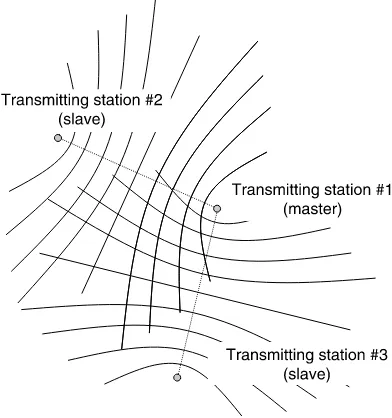
As local time generators (oscillators or atomic clocks) were evolving rapidly, new uses of radio signals were developed. This was the case for hyperbolic systems. The basic principle states that all locations having the same difference of signal travel time to two ﬁxed points, for instance two radio transmitters, lie on a geometrical ﬁgure that is a hyperbola. The focal points of this hyperbola are the transmitters. As

7_{Goniometry is the way of measuring the angle of rotation of the aerial of a wireless system in order to}

obtain the direction of arrival of the radio wave.

(37)

signal-processing capabilities increased, such time difference estimations and measurements became possible. Note that synchronization at the mobile receiver’s end is thus avoided as long as time differences are carried out. The basic idea was to obtain two such differences in order to allow the calculation of the intersection point of the resulting two hyperbolae (Fig. 1.13). This approach leads to a theoretical single point in a two-dimensional space.

The ﬁrst system that used this technique was the Decca,8 which came into

operation at the end of World War II. It worked within a frequency band of 70 – 128 kHz, allowing for approximately 450 km of operational range. The resulting accuracy was in the range of a few hundred meters, depending on propagation conditions. The new era of radio electric signals allowed for a rigorous evaluation of accuracy — a very important parameter.

The current e-Loran9is also a hyperbolic system, but which added new features

concerning the modulation scheme, based on pulse trains forwarded by each master

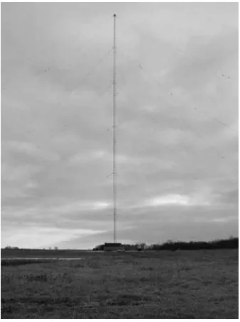
and slave station.10This approach allowed for a more precise positioning, together

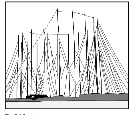
with an efﬁcient way of identifying the various stations. The frequency band used was ﬁrst in the 1750 – 1950 kHz range for LORAN-A, and is currently in the 90 – 110 kHz range for eLoran (which is the latest development of LORAN-C). This fre-quency involves the use of very large antennas (Fig. 1.14) in order to achieve long range and high power transmission.

FIGURE 1.13 Representation of the hyperbolic approach.

8_{Proposed by the Decca Navigator Company.} 9_{Enhanced LOng RAnge Navigation system.}

10_{The master station is the one that masters the time. The slave stations have to be synchronized with the}

master station.

(38)

These first terrestrial systems provided what is termed “local” area coverage, even though this coverage can be quite large (this is the case for LORAN). However, some people imagined an even more ambitious project that would be the ultimate version of a terrestrial system with a global coverage: the Omega system. It was made up of eight stations using a very low frequency (VLF) band in order to have a complete coverage of the Earth. It was still a hyperbolic approach; each station transmitted sequentially, always in the same order for about 1 s (the duration of emission is specific to each station). The emission consisted of pure con-tinuous waves (no modulation scheme) at respectively 10.2, 11.33, and 13.6 kHz. The sequencing of transmission of these three frequencies was also specific to each station. The total polling sequence lasted 10 s, and the synchronization was

required to be better than 1ms. To calculate an accurate location, it was also

necess-ary to apply propagation corrections. These were based on long-period (typically 15 days) corrections depending on the date, the time of the day, and also on the esti-mated location. Once more, as we shall see later, the modern principle of satellite constellations was already present, only without the satellite aspects. The global accuracy was generally better than 8 km.

The major reason for the poor accuracy of the abovementioned systems is included in propagation modeling (this point has constantly driven the evolution of modern systems). A new system was designed in order to reduce the propagation errors, and was called the differential Omega. The idea was simply to consider a receiver located in a well-known position, and which monitored the difference between the calculated location and the actual one. This difference was used as an error vector that could be subtracted from the calculated location of any receiver

FIGURE 1.14 A typical LORAN antenna. (Source: Megapulse.)

(39)

that encountered the same propagation conditions, that is, which was located in the vicinity of the ﬁxed reference receiver. Using this differential approach, the accuracy dropped down to 1.5 km, as long as the receiver remained within about 450 km of the ﬁxed reference; that is, the propagation conditions remained almost identical. The reader should note that this approach was also deployed with the Global Positioning System (GPS) when the U.S. government attached a deliberately generated error, the so-called Selective Availability (which was switched off on May 1, 2000).

Besides these global coverage systems, some speciﬁc systems are locally deployed, such as the VOR (VHF Omnidirectional Radio Range) or TACAN (Tactical Air Navigation), as well as others such as ILS (Instrument Landing System) and MLS (Microwave Landing System). All these systems were developed for air navigation purposes, in order to provide the locations of aircraft relative to ground facilities. The VOR is essentially a rotating radio lighthouse and has a medium distance range. The frequency of transmission lies between 108 and 118 MHz, and the signal is modulated in such a way that the transmission is composed of two simultaneous and independent signals at 30 Hz, whose difference of phase characterizes the azimuth of the receiver. In order to achieve this, the VOR radiates at a variable 30 Hz with a symmetric radiating diagram exhibiting a cardioid pattern. Simultaneously, the second signal is a 30 Hz uniform (omnidirectional

pattern) signal whose phase is identical in all directions.11The onboard receiver

cal-culates the direction of the VOR station, but also selects an azimuth route for a direc-tion chosen by a user. If this direcdirec-tion is the VOR stadirec-tion, then the phase difference signal should be zero. Thus, an indication of the deviation between the real route and the VOR station direction can be provided. Such equipment could be used for posi-tioning, as long as three VOR stations are in radio visibility, by achieving a triangu-lation from the three directions of arrival measurements. As a matter of fact, this system is mainly used as an alignment device and is usually associated with DME (Distance Measuring Equipment), which gives the distance between the device and a reference ground station. An association between VOR and DME thus gives the plane’s location (in polar coordinates) in the ground station referential. The range is typically 200 miles in good conditions and the accuracy lies around 0.2 miles or 0.25% of the measured distance. The military extrapolation of VOR and DME is the TACAN system, which includes both functions on the same carrier frequency.

The accuracy of such a system is nevertheless not enough to provide aviation with an all-weather landing system. Thus, the ILS and MLS were developed. The first is composed of two rotating radio lighthouses that respectively define a direction (the alignment of the runway) and an angle of approach. The first uses frequencies in the range 108 – 112 kHz and the second 328 – 335 MHz. Because of the use of these frequencies, multipath effects can occur and trouble the angle measurements. In addition, the system also includes two or three “markers” (radio beacons), which radiate vertically and are distance markers on the approach to the runway. The MLS was seen as the solution to this problem; it used a high-frequency (5 GHz) narrow rotating beam (1 – 38) in order to scan space.

(40)

In addition to the abovementioned systems, there are some other local systems that implement either hyperbolic approaches (Hi-Fix, Sea-Fix, Raydist, Lorac, Toran, and so on) or circular approaches (Mini Ranger, Micro-Fix, Trisponder, Tellurometre, Geodimeter, Syladis, Axyle, and so on). The hyperbolic systems almost exclusively use the 1.6 – 3 MHz band. The corresponding wavelength, when compared to LORAN for instance, allowed much better measurement accuracy, to the order of a few meters. Carrier phase measurements were carried out, and an ambi-guity (distance error of half the wavelength) was required to be removed by speciﬁc methods (not described here). In the case of circular systems, positioning is obtained using intersecting circles (and no longer hyperbolae) as direct distance measurements are carried out and there is no longer the need for establishing the difference. These systems were called “range – range” and the use of higher frequencies allowed frequency modulation to be developed, notably in relation to code sequences, which permitted the ambiguity problem to be reduced.

B

1.6 THE ERA OF ARTIFICIAL SATELLITES

In the late 1920s, physicians and mathematicians showed that it was theoretically feasible to imagine artificial satellites launched from the Earth’s surface and orbiting the Earth. Of course, a lot of research was still required, but it was thought possible. In 1952, the International Council of Scientific Unions decided that from July 1, 1957, to the end of 1958 would be the “International Geophysical Year (IGY).” The main reason for this choice was that the astrophysical activity of the Sun and a few other stars would be of spectacular importance, thus allowing a large number of valuable research activities. In October 1954, the Council adopted a resolution calling for arti-ficial satellite launches during the abovementioned IGY. One has to remember that this was the time of the Cold War between the United States and the Soviet Union; the proposition was a new area of competition, this time scientific, between the nations. In July 1955, the White House announced its wish to make such a launch and issued a call for projects. In September 1955, the Vanguard project (Fig. 1.15), proposed by the Naval Research Laboratory, was selected among others to represent the United States.

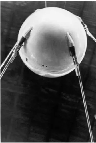
On October 4, 1957, the Soviet Union launched Sputnik-1 (Fig. 1.16), called the “basket ball,” weighing 183 lb, on an elliptic orbit with a 98-min revolution period. The Soviet Union also launched Sputnik-2 on November 3, 1957, with the dog Laika onboard. On October 23, 1957, tests were carried out on the Vanguard launcher, which broke down on 6 December at the time of launching.

On 31 January, 1958, the United States launched Explorer-1 (Fig. 1.17), the new project, using a Jupiter C launcher, developed by a U.S. Army team led by Wernher von Braun. Explorer-1 had a mass of 13.9 kg, and would discover the Van Allen radiating belts.12

12_{The Van Allen belts are charged particle belts linked to the presence of the Earth’s magnetic ﬁeld and are}

located around the Earth.

(41)

FIGURE 1.15 The Vanguard project (the satellite was called the “grapefruit”). (Source: NASA.)

FIGURE 1.16 Sputnik, called the “basket ball.” (Source: NASA.)

(42)

Let us come back to the ﬁrst Sputnik launch. To prove that a satellite was actually orbiting the Earth, it was planned that it should transmit a signal. Sputnik used a 400 MHz carrier frequency with sound modulation data. In such a way, once

demo-dulated, it was possible to “hear” Sputnik.13 Nothing was really known about this

ﬂight — the orbit, the speed of the satellite, the duration of the transmission, and so on. So, it was a fantastic opportunity to carry out some tests. Among others, George C. Weiffenbach and William H. Guier, members of the Applied Physics Laboratory of the Johns Hopkins University, carried out such investigations. They

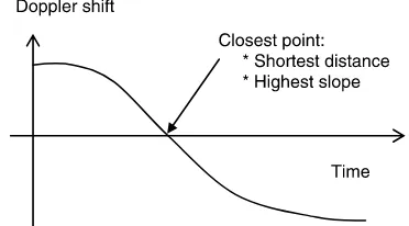
succeeded in determining Sputnik’s orbit by analyzing the Doppler shift14 of the

signal while the satellite was in radio visibility, that is, for about 40 min of the 108 min of a complete revolution of Sputnik.

The method they used to achieve such a goal was of fundamental importance as it is the starting point of all modern satellite navigation systems. The measurement was of the Doppler shift, the unknown variable was the orbit of the satellite, and another piece of data was the actual location of the place of observation (that is, the labora-tory). After about three weeks of observation and a few calculations, they ﬁnally showed that it was possible to calculate the orbit, knowing both the Doppler shift

FIGURE 1.17 The Explorer 1 project. (Source: NASA.)

13_{What was then “hearable” can be listened to at www.amsat.org}

/amsat/features/sounds/ﬁrstsat.html.

14_{The Doppler shift is the physical phenomenon that shifts the frequency of any wave transmitted,}

depend-ing on the relative speed between the transmitter and the receiver. Let us deﬁneDas the distance between the transmitter and the receiver: the frequency received is increased whenDdecreases and decreased when

Dincreases. Note that this phenomenon is a physical time compression of the signal and applies to all waves (sound, radio, light, and so on).