Programming Computer Vision
with Python
Jan Erik Solem
Programming Computer Vision with Python by Jan Erik Solem
Copyright © 2012 Jan Erik Solem. All rights reserved. Printed in the United States of America
Published by O’Reilly Media, Inc., 1005 Gravenstein Highway North, Sebastopol, CA 95472.
O’Reilly books may be purchased for educational, business, or sales promotional use. Online editions are also available for most titles (http://my.safaribooksonline.com). For more information, contact our corporate/institutional sales department: (800) 998-9938 or[email protected].
Interior designer: David Futato Project manager: Paul C. Anagnostopoulos Cover designer: Karen Montgomery Copyeditor: Priscilla Stevens
Editors: Andy Oram, Mike Hendrickson Proofreader: Richard Camp Production editor: Holly Bauer Illustrator: Laurel Muller June 2012 First edition
Revision History for the First Edition: 2012-06-11 First release
Seehttp://oreilly.com/catalog/errata.csp?isbn=0636920022923for release details.
Nutshell Handbook, the Nutshell Handbook logo, and the O’Reilly logo are registered trademarks of O’Reilly Media, Inc.Programming Computer Vision with Python, the image of a bullhead fish, and related trade dress are trademarks of O’Reilly Media, Inc.
Many of the designations used by manufacturers and sellers to distinguish their products are claimed as trademarks. Where those designations appear in this book, and O’Reilly Media, Inc., was aware of a trademark claim, the designations have been printed in caps or initial caps.
While every precaution has been taken in the preparation of this book, the publisher and authors assume no responsibility for errors or omissions, or for damages resulting from the use of the information contained herein.
Table of Contents
Preface . . . vii
1. Basic Image Handling and Processing . . . 1
1.1 PIL—The Python Imaging Library 1
1.2 Matplotlib 3
1.3 NumPy 7
1.4 SciPy 16
1.5 Advanced Example: Image De-Noising 23
Exercises 26
Conventions for the Code Examples 27
2. Local Image Descriptors . . . 29
2.1 Harris Corner Detector 29
2.2 SIFT—Scale-Invariant Feature Transform 36
2.3 Matching Geotagged Images 44
Exercises 51
3. Image to Image Mappings . . . 53
3.1 Homographies 53
3.2 Warping Images 57
3.3 Creating Panoramas 70
Exercises 77
4. Camera Models and Augmented Reality . . . 79
4.1 The Pin-Hole Camera Model 79
4.2 Camera Calibration 84
4.3 Pose Estimation from Planes and Markers 86
4.4 Augmented Reality 89
Exercises 98
5. Multiple View Geometry . . . 99
5.1 Epipolar Geometry 99
5.2 Computing with Cameras and 3D Structure 107
5.3 Multiple View Reconstruction 113
5.4 Stereo Images 120
Exercises 125
6. Clustering Images . . . 127
6.1 K-Means Clustering 127
6.2 Hierarchical Clustering 133
6.3 Spectral Clustering 140
Exercises 145
7. Searching Images . . . 147
7.1 Content-Based Image Retrieval 147
7.2 Visual Words 148
7.3 Indexing Images 151
7.4 Searching the Database for Images 155
7.5 Ranking Results Using Geometry 160
7.6 Building Demos and Web Applications 162
Exercises 165
8. Classifying Image Content . . . 167
8.1 K-Nearest Neighbors 167
8.2 Bayes Classifier 175
8.3 Support Vector Machines 179
8.4 Optical Character Recognition 183
Exercises 189
9. Image Segmentation . . . 191
9.1 Graph Cuts 191
9.2 Segmentation Using Clustering 200
9.3 Variational Methods 204
Exercises 206
10. OpenCV . . . 209
10.1 The OpenCV Python Interface 209
10.2 OpenCV Basics 210
10.3 Processing Video 213
10.4 Tracking 216
10.5 More Examples 223
A. Installing Packages . . . 227
A.1 NumPy and SciPy 227
A.2 Matplotlib 228
A.3 PIL 228
A.4 LibSVM 228
A.5 OpenCV 229
A.6 VLFeat 230
A.7 PyGame 230
A.8 PyOpenGL 230
A.9 Pydot 230
A.10 Python-graph 231
A.11 Simplejson 231
A.12 PySQLite 232
A.13 CherryPy 232
B. Image Datasets . . . 233
B.1 Flickr 233
B.2 Panoramio 234
B.3 Oxford Visual Geometry Group 235
B.4 University of Kentucky Recognition Benchmark Images 235
B.5 Other 235
C. Image Credits . . . 237
C.1 Images from Flickr 237
C.2 Other Images 238
C.3 Illustrations 238
References . . . 239
Index . . . 243
Preface
Today, images and video are everywhere. Online photo-sharing sites and social net-works have them in the billions. Search engines will produce images of just about any conceivable query. Practically all phones and computers come with built-in cameras. It is not uncommon for people to have many gigabytes of photos and videos on their devices.
Programming a computer and designing algorithms for understanding what is in these images is the field of computer vision. Computer vision powers applications like image search, robot navigation, medical image analysis, photo management, and many more. The idea behind this book is to give an easily accessible entry point to hands-on computer vision with enough understanding of the underlying theory and algorithms to be a foundation for students, researchers, and enthusiasts. The Python programming language, the language choice of this book, comes with many freely available, powerful modules for handling images, mathematical computing, and data mining.
When writing this book, I have used the following principles as a guideline. The book should:
. Be written in an exploratory style and encourage readers to follow the examples on
their computers as they are reading the text.
. Promote and use free and open software with a low learning threshold. Python was
the obvious choice.
. Be complete and self-contained. This book does not cover all of computer vision
but rather it should be complete in that all code is presented and explained. The reader should be able to reproduce the examples and build upon them directly.
. Be broad rather than detailed, inspiring and motivational rather than theoretical.
In short, it should act as a source of inspiration for those interested in programming computer vision applications.
Prerequisites and Overview
This book looks at theory and algorithms for a wide range of applications and problems. Here is a short summary of what to expect.
What You Need to Know
. Basic programming experience. You need to know how to use an editor and run
scripts, how to structure code as well as basic data types. Familiarity with Python or other scripting languages like Ruby or Matlab will help.
. Basic mathematics. To make full use of the examples, it helps if you know about
matrices, vectors, matrix multiplication, and standard mathematical functions and concepts like derivatives and gradients. Some of the more advanced mathematical examples can be easily skipped.
What You Will Learn
. Hands-on programming with images using Python.
. Computer vision techniques behind a wide variety of real-world applications. . Many of the fundamental algorithms and how to implement and apply them
yourself.
The code examples in this book will show you object recognition, content-based image retrieval, image search, optical character recognition, optical flow, tracking, 3D reconstruction, stereo imaging, augmented reality, pose estimation, panorama creation, image segmentation, de-noising, image grouping, and more.
Chapter Overview
Chapter 1, “Basic Image Handling and Processing”
Introduces the basic tools for working with images and the central Python modules used in the book. This chapter also covers many fundamental examples needed for the remaining chapters.
Chapter 2, “Local Image Descriptors”
Explains methods for detecting interest points in images and how to use them to find corresponding points and regions between images.
Chapter 3, “Image to Image Mappings”
Describes basic transformations between images and methods for computing them. Examples range from image warping to creating panoramas.
Chapter 4, “Camera Models and Augmented Reality”
Introduces how to model cameras, generate image projections from 3D space to image features, and estimate the camera viewpoint.
Chapter 5, “Multiple View Geometry”
Chapter 6, “Clustering Images”
Introduces a number of clustering methods and shows how to use them for group-ing and organizgroup-ing images based on similarity or content.
Chapter 7, “Searching Images”
Shows how to build efficient image retrieval techniques that can store image rep-resentations and search for images based on their visual content.
Chapter 8, “Classifying Image Content”
Describes algorithms for classifying image content and how to use them to recog-nize objects in images.
Chapter 9, “Image Segmentation”
Introduces different techniques for dividing an image into meaningful regions using clustering, user interactions, or image models.
Chapter 10, “OpenCV”
Shows how to use the Python interface for the commonly used OpenCV computer vision library and how to work with video and camera input.
There is also a bibliography at the back of the book. Citations of bibliographic entries are made by number in square brackets, as in [20].
Introduction to Computer Vision
Computer vision is the automated extraction of information from images. Information can mean anything from 3D models, camera position, object detection and recognition to grouping and searching image content. In this book, we take a wide definition of computer vision and include things like image warping, de-noising, and augmented reality.1
Sometimes computer vision tries to mimic human vision, sometimes it uses a data and statistical approach, and sometimes geometry is the key to solving problems. We will try to cover all of these angles in this book.
Practical computer vision contains a mix of programming, modeling, and mathematics and is sometimes difficult to grasp. I have deliberately tried to present the material with a minimum of theory in the spirit of “as simple as possible but no simpler.” The mathematical parts of the presentation are there to help readers understand the algorithms. Some chapters are by nature very math-heavy (Chapters 4 and 5, mainly). Readers can skip the math if they like and still use the example code.
Python and NumPy
Python is the programming language used in the code examples throughout this book. Python is a clear and concise language with good support for input/output, numer-ics, images, and plotting. The language has some peculiarities, such as indentation
1These examples produce new images and are more image processing than actually extracting information from
images.
and compact syntax, that take getting used to. The code examples assume you have Python 2.6 or later, as most packages are only available for these versions. The upcom-ing Python 3.x version has many language differences and is not backward compatible with Python 2.x or compatible with the ecosystem of packages we need (yet).
Some familiarity with basic Python will make the material more accessible for read-ers. For beginners to Python, Mark Lutz’ bookLearning Python[20] and the online documentation athttp://www.python.org/are good starting points.
When programming computer vision, we need representations of vectors and matrices and operations on them. This is handled by Python’sNumPymodule, where both vectors and matrices are represented by thearraytype. This is also the representation we will use for images. A goodNumPyreference is Travis Oliphant’s free bookGuide to NumPy
[24]. The documentation athttp://numpy.scipy.org/is also a good starting point if you are new toNumPy. For visualizing results, we will use theMatplotlibmodule, and for more advanced mathematics, we will useSciPy. These are the central packages you will need and will be explained and introduced in Chapter 1.
Besides these central packages, there will be many other free Python packages used for specific purposes like reading JSON or XML, loading and saving data, generating graphs, graphics programming, web demos, classifiers, and many more. These are usually only needed for specific applications or demos and can be skipped if you are not interested in that particular application.
It is worth mentioning IPython, an interactive Python shell that makes debugging and experimentation easier. Documentation and downloads are available at
http://ipython.org/.
Notation and Conventions
Code looks like this: # some points x = [100,100,400,400] y = [200,500,200,500]
# plot the points
plot(x,y)
The following typographical conventions are used in this book:
Italic
Used for definitions, filenames, and variable names.
Constant width
Used for functions, Python modules, and code examples. It is also used for console printouts.
Hyperlink
Used for URLs. Plain text
Mathematical formulas are given inline like thisf (x)=wTx+bor centered
indepen-dently:
f (x)=
i
wixi+b
and are only numbered when a reference is needed.
In the mathematical sections, we will use lowercase (s,r,λ,θ, . . .) for scalars, upper-case (A,V,H, . . .) for matrices (includingI for the image as an array), and lowercase bold (t,c, . . .) for vectors. We will usex=[x,y] andX=[X,Y,Z] to mean points in 2D (images) and 3D, respectively.
Using Code Examples
This book is here to help you get your job done. In general, you may use the code in this book in your programs and documentation. You do not need to contact us for permission unless you’re reproducing a significant portion of the code. For example, writing a program that uses several chunks of code from this book does not require permission. Selling or distributing a CD-ROM of examples from O’Reilly books does require permission. Answering a question by citing this book and quoting example code does not require permission. Incorporating a significant amount of example code from this book into your product’s documentation does require permission.
We appreciate, but do not require, attribution. An attribution usually includes the title, author, publisher, and ISBN. For example: “Programming Computer Vision with Python
by Jan Erik Solem (O’Reilly). Copyright © 2012 Jan Erik Solem, 978-1-449-31654-9.” If you feel your use of code examples falls outside fair use or the permission given above, feel free to contact us at[email protected].
How to Contact Us
Please address comments and questions concerning this book to the publisher: O’Reilly Media, Inc.
1005 Gravenstein Highway North Sebastopol, CA 95472
(800) 998-9938 (in the United States or Canada) (707) 829-0515 (international or local)
(707) 829-0104 (fax)
We have a web page for this book, where we list errata, examples, links to the code and data sets used, and any additional information. You can access this page at:
oreil.ly/comp_vision_w_python
To comment or ask technical questions about this book, send email to:
For more information about our books, courses, conferences, and news, see our website athttp://www.oreilly.com.
Find us on Facebook:http://facebook.com/oreilly
Follow us on Twitter:http://twitter.com/oreillymedia
Watch us on YouTube:http://www.youtube.com/oreillymedia
Safari® Books Online
Safari Books Online (www.safaribooksonline.com) is an on-demand digital library that delivers expert content in both book and video form from the world’s leading authors in technology and business.
Technology professionals, software developers, web designers, and business and cre-ative professionals use Safari Books Online as their primary resource for research, problem solving, learning, and certification training.
Safari Books Online offers a range of product mixes and pricing programs for organi-zations, government agencies, and individuals. Subscribers have access to thousands of books, training videos, and prepublication manuscripts in one fully searchable data-base from publishers like O’Reilly Media, Prentice Hall Professional, Addison-Wesley Professional, Microsoft Press, Sams, Que, Peachpit Press, Focal Press, Cisco Press, John Wiley & Sons, Syngress, Morgan Kaufmann, IBM Redbooks, Packt, Adobe Press, FT Press, Apress, Manning, New Riders, McGraw-Hill, Jones & Bartlett, Course Technol-ogy, and dozens more. For more information about Safari Books Online, please visit us online.
Acknowledgments
I’d like to express my gratitude to everyone involved in the development and production of this book. The whole O’Reilly team has been helpful. Special thanks to Andy Oram (O’Reilly) for editing, and Paul Anagnostopoulos (Windfall Software) for efficient production work.
CHAPTER 1
Basic Image Handling
and Processing
This chapter is an introduction to handling and processing images. With extensive examples, it explains the central Python packages you will need for working with images. This chapter introduces the basic tools for reading images, converting and scaling images, computing derivatives, plotting or saving results, and so on. We will use these throughout the remainder of the book.
1.1 PIL—The Python Imaging Library
ThePython Imaging Library(PIL) provides general image handling and lots of useful basic image operations like resizing, cropping, rotating, color conversion and much more. PIL is free and available fromhttp://www.pythonware.com/products/pil/.
With PIL, you can read images from most formats and write to the most common ones. The most important module is theImagemodule. To read an image, use:
from PIL import Image
pil_im = Image.open('empire.jpg')
The return value,pil_im, is a PIL image object.
Color conversions are done using theconvert()method. To read an image and convert it to grayscale, just addconvert('L')like this:
pil_im = Image.open('empire.jpg').convert('L')
Here are some examples taken from the PIL documentation, available athttp://www .pythonware.com/library/pil/handbook/index.htm. Output from the examples is shown in Figure 1-1.
Convert Images to Another Format
Using thesave()method, PIL can save images in most image file formats. Here’s an example that takes all image files in a list of filenames (filelist) and converts the images to JPEG files:
Figure 1-1. Examples of processing images with PIL.
from PIL import Image import os
for infile in filelist:
outfile = os.path.splitext(infile)[0] + ".jpg" if infile != outfile:
try:
Image.open(infile).save(outfile) except IOError:
print "cannot convert", infile
The PIL functionopen()creates a PIL image object and thesave()method saves the image to a file with the given filename. The new filename will be the same as the original with the file ending “.jpg” instead. PIL is smart enough to determine the image format from the file extension. There is a simple check that the file is not already a JPEG file and a message is printed to the console if the conversion fails.
Throughout this book we are going to need lists of images to process. Here’s how you could create a list of filenames of all images in a folder. Create a file calledimtools.pyto store some of these generally useful routines and add the following function:
import os
def get_imlist(path):
""" Returns a list of filenames for all jpg images in a directory. """
return [os.path.join(path,f) for f in os.listdir(path) if f.endswith('.jpg')] Now, back to PIL.
Create Thumbnails
within the tuple. To create a thumbnail with longest side 128 pixels, use the method like this:
pil_im.thumbnail((128,128))
Copy and Paste Regions
Cropping a region from an image is done using thecrop()method: box = (100,100,400,400)
region = pil_im.crop(box)
The region is defined by a 4-tuple, where coordinates are (left, upper, right, lower). PIL uses a coordinate system with(0, 0)in the upper left corner. The extracted region can, for example, be rotated and then put back using thepaste()method like this:
region = region.transpose(Image.ROTATE_180) pil_im.paste(region,box)
Resize and Rotate
To resize an image, callresize()with a tuple giving the new size: out = pil_im.resize((128,128))
To rotate an image, use counterclockwise angles androtate()like this: out = pil_im.rotate(45)
Some examples are shown in Figure 1-1. The leftmost image is the original, followed by a grayscale version, a rotated crop pasted in, and a thumbnail image.
1.2 Matplotlib
When working with mathematics and plotting graphs or drawing points, lines, and curves on images, Matplotlib is a good graphics library with much more powerful features than the plotting available in PIL.Matplotlibproduces high-quality figures like many of the illustrations used in this book. Matplotlib’s PyLabinterface is the set of functions that allows the user to create plots. Matplotlib is open source and available freely fromhttp://matplotlib.sourceforge.net/, where detailed documentation and tutorials are available. Here are some examples showing most of the functions we will need in this book.
Plotting Images, Points, and Lines
Although it is possible to create nice bar plots, pie charts, scatter plots, etc., only a few commands are needed for most computer vision purposes. Most importantly, we want to be able to show things like interest points, correspondences, and detected objects using points and lines. Here is an example of plotting an image with a few points and a line:
from PIL import Image from pylab import *
# read image to array
im = array(Image.open('empire.jpg'))
# plot the image
imshow(im)
# some points
x = [100,100,400,400] y = [200,500,200,500]
# plot the points with red star-markers
plot(x,y,'r*')
# line plot connecting the first two points
plot(x[:2],y[:2])
# add title and show the plot
title('Plotting: "empire.jpg"') show()
This plots the image, then four points with red star markers at the x and y coordinates given by thexandylists, and finally draws a line (blue by default) between the two first points in these lists. Figure 1-2 shows the result. Theshow()command starts the figure GUI and raises the figure windows. This GUI loop blocks your scripts and they are paused until the last figure window is closed. You should callshow()only once per script, usually at the end. Note thatPyLabuses a coordinate origin at the top left corner as is common for images. The axes are useful for debugging, but if you want a prettier plot, add:
axis('off')
This will give a plot like the one on the right in Figure 1-2 instead.
There are many options for formatting color and styles when plotting. The most useful are the short commands shown in Tables 1-1, 1-2 and 1-3. Use them like this:
plot(x,y) # default blue solid line
plot(x,y,'r*') # red star-markers
plot(x,y,'go-') # green line with circle-markers
plot(x,y,'ks:') # black dotted line with square-markers
Image Contours and Histograms
Figure 1-2. Examples of plotting withMatplotlib. An image with points and a line with and without showing the axes.
Table 1-1. Basic color formatting commands for plotting withPyLab.
Color
'b' blue
'g' green
'r' red 'c' cyan
'm' magenta
'y' yellow
'k' black
'w' white
Table 1-2. Basic line style formatting commands for plotting withPyLab.
Line style
'-' solid
'- -' dashed
':' dotted
Table 1-3. Basic plot marker formatting commands for plotting withPyLab.
Marker
'.' point
'o' circle
's' square
'*' star '+' plus
'x' x
useful. This needs grayscale images, because the contours need to be taken on a single value for every coordinate [x,y]. Here’s how to do it:
from PIL import Image from pylab import *
# read image to array
im = array(Image.open('empire.jpg').convert('L'))
# create a new figure
figure()
# don't use colors
gray()
# show contours with origin upper left corner
contour(im, origin='image') axis('equal')
axis('off')
As before, the PIL methodconvert()does conversion to grayscale.
An image histogram is a plot showing the distribution of pixel values. A number of bins is specified for the span of values and each bin gets a count of how many pixels have values in the bin’s range. The visualization of the (graylevel) image histogram is done using thehist()function:
figure()
hist(im.flatten(),128) show()
The second argument specifies the number of bins to use. Note that the image needs to be flattened first, becausehist()takes a one-dimensional array as input. The method
flatten()converts any array to a one-dimensional array with values taken row-wise. Figure 1-3 shows the contour and histogram plot.
Interactive Annotation
Sometimes users need to interact with an application, for example by marking points in an image, or you need to annotate some training data.PyLabcomes with a simple function,ginput(), that lets you do just that. Here’s a short example:
from PIL import Image from pylab import *
im = array(Image.open('empire.jpg')) imshow(im)
print 'Please click 3 points' x = ginput(3)
print 'you clicked:',x show()
This plots an image and waits for the user to click three times in the image region of the figure window. The coordinates [x,y] of the clicks are saved in a listx.
1.3 NumPy
NumPy(http://www.scipy.org/NumPy/) is a package popularly used for scientific comput-ing with Python.NumPycontains a number of useful concepts such as array objects (for representing vectors, matrices, images and much more) and linear algebra functions. TheNumPyarray object will be used in almost all examples throughout this book.1The array object lets you do important operations such as matrix multiplication, transpo-sition, solving equation systems, vector multiplication, and normalization, which are needed to do things like aligning images, warping images, modeling variations, classi-fying images, grouping images, and so on.
NumPyis freely available fromhttp://www.scipy.org/Downloadand the online documen-tation (http://docs.scipy.org/doc/numpy/) contains answers to most questions. For more details onNumPy, the freely available book [24] is a good reference.
Array Image Representation
When we loaded images in the previous examples, we converted them toNumPyarray objects with thearray()call but didn’t mention what that means. Arrays inNumPyare multi-dimensional and can represent vectors, matrices, and images. An array is much like a list (or list of lists) but is restricted to having all elements of the same type. Unless specified on creation, the type will automatically be set depending on the data. The following example illustrates this for images:
im = array(Image.open('empire.jpg')) print im.shape, im.dtype
im = array(Image.open('empire.jpg').convert('L'),'f') print im.shape, im.dtype
1PyLabactually includes some components ofNumPy, like the array type. That’s why we could use it in the
examples in Section 1.2.
The printout in your console will look like this: (800, 569, 3) uint8
(800, 569) float32
The first tuple on each line is the shape of the image array (rows, columns, color channels), and the following string is the data type of the array elements. Images are usually encoded with unsigned 8-bit integers (uint8), so loading this image and converting to an array gives the type “uint8” in the first case. The second case does grayscale conversion and creates the array with the extra argument “f”. This is a short command for setting the type to floating point. For more data type options, see [24]. Note that the grayscale image has only two values in the shape tuple; obviously it has no color information.
Elements in the array are accessed with indexes. The value at coordinatesi,jand color channelkare accessed like this:
value = im[i,j,k]
Multiple elements can be accessed using array slicing.Slicingreturns a view into the array specified by intervals. Here are some examples for a grayscale image:
im[i,:] = im[j,:] # set the values of row i with values from row j
im[:,i] = 100 # set all values in column i to 100
im[:100,:50].sum() # the sum of the values of the first 100 rows and 50 columns
im[50:100,50:100] # rows 50-100, columns 50-100 (100th not included)
im[i].mean() # average of row i
im[:,-1] # last column
im[-2,:] (or im[-2]) # second to last row
Note the example with only one index. If you only use one index, it is interpreted as the row index. Note also the last examples. Negative indices count from the last element backward. We will frequently use slicing to access pixel values, and it is an important concept to understand.
There are many operations and ways to use arrays. We will introduce them as they are needed throughout this book. See the online documentation or the book [24] for more explanations.
Graylevel Transforms
After reading images toNumPyarrays, we can perform any mathematical operation we like on them. A simple example of this is to transform the graylevels of an image. Take any functionfthat maps the interval 0 . . . 255 (or, if you like, 0 . . . 1) to itself (meaning that the output has the same range as the input). Here are some examples:
from PIL import Image from numpy import *
im = array(Image.open('empire.jpg').convert('L'))
im3 = (100.0/255) * im + 100 # clamp to interval 100...200
im4 = 255.0 * (im/255.0)**2 # squared
The first example inverts the graylevels of the image, the second one clamps the intensi-ties to the interval 100 . . . 200, and the third applies a quadratic function, which lowers the values of the darker pixels. Figure 1-4 shows the functions and Figure 1-5 the result-ing images. You can check the minimum and maximum values of each image usresult-ing:
print int(im.min()), int(im.max())
Figure 1-4. Example of graylevel transforms. Three example functions together with the identity transform showed as a dashed line.
Figure 1-5. Graylevel transforms. Applying the functions in Figure 1-4: Inverting the image with f (x)=255−x (left), clamping the image withf (x)=(100/255)x+100(middle), quadratic transformation withf (x)=255(x/255)2(right).
If you try that for each of the examples above, you should get the following output: 2 255
0 253 100 200 0 255
The reverse of the array() transformation can be done using the PIL function
fromarray()as:
pil_im = Image.fromarray(im)
If you did some operation to change the type from “uint8” to another data type, such asim3orim4in the example above, you need to convert back before creating the PIL image:
pil_im = Image.fromarray(uint8(im))
If you are not absolutely sure of the type of the input, you should do this as it is the safe choice. Note thatNumPywill always change the array type to the “lowest” type that can represent the data. Multiplication or division with floating point numbers will change an integer type array to float.
Image Resizing
NumPyarrays will be our main tool for working with images and data. There is no simple way to resize arrays, which you will want to do for images. We can use the PIL image object conversion shown earlier to make a simple image resizing function. Add the following toimtools.py:
def imresize(im,sz):
""" Resize an image array using PIL. """
pil_im = Image.fromarray(uint8(im))
return array(pil_im.resize(sz)) This function will come in handy later.
Histogram Equalization
A very useful example of a graylevel transform ishistogram equalization. This transform flattens the graylevel histogram of an image so that all intensities are as equally common as possible. This is often a good way to normalize image intensity before further processing and also a way to increase image contrast.
The transform function is, in this case, acumulative distribution function(cdf) of the pixel values in the image (normalized to map the range of pixel values to the desired range).
Here’s how to do it. Add this function to the fileimtools.py: def histeq(im,nbr_bins=256):
# get image histogram
imhist,bins = histogram(im.flatten(),nbr_bins,normed=True) cdf = imhist.cumsum()# cumulative distribution function
cdf = 255 * cdf / cdf[-1] # normalize
# use linear interpolation of cdf to find new pixel values
im2 = interp(im.flatten(),bins[:-1],cdf)
return im2.reshape(im.shape), cdf
The function takes a grayscale image and the number of bins to use in the histogram as input, and returns an image with equalized histogram together with the cumulative distribution function used to do the mapping of pixel values. Note the use of the last element (index -1) of the cdf to normalize it between 0 . . . 1. Try this on an image like this:
from PIL import Image from numpy import *
im = array(Image.open('AquaTermi_lowcontrast.jpg').convert('L')) im2,cdf = imtools.histeq(im)
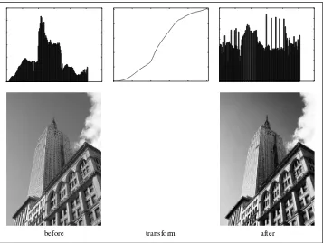
Figures 1-6 and 1-7 show examples of histogram equalization. The top row shows the graylevel histogram before and after equalization together with the cdf mapping. As you can see, the contrast increases and the details of the dark regions now appear clearly.
Averaging Images
Averaging images is a simple way of reducing image noise and is also often used for artistic effects. Computing an average image from a list of images is not difficult. Assuming the images all have the same size, we can compute the average of all those images by simply summing them up and dividing with the number of images. Add the following function toimtools.py:
def compute_average(imlist):
""" Compute the average of a list of images. """ # open first image and make into array of type float
averageim = array(Image.open(imlist[0]), 'f')
for imname in imlist[1:]: try:
averageim += array(Image.open(imname)) except:
print imname + '...skipped' averageim /= len(imlist)
# return average as uint8
return array(averageim, 'uint8')
This includes some basic exception handling to skip images that can’t be opened. There is another way to compute average images using themean()function. This requires all images to be stacked into an array and will use lots of memory if there are many images. We will use this function in the next section.
before transform after
Figure 1-6. Example of histogram equalization. On the left is the original image and histogram. The middle plot is the graylevel transform function. On the right is the image and histogram after histogram equalization.
before transform after
PCA of Images
Principal Component Analysis(PCA) is a useful technique for dimensionality reduction and is optimal in the sense that it represents the variability of the training data with as few dimensions as possible. Even a tiny 100×100 pixel grayscale image has 10,000 dimensions, and can be considered a point in a 10,000-dimensional space. A megapixel image has dimensions in the millions. With such high dimensionality, it is no surprise that dimensionality reduction comes in handy in many computer vision applications. The projection matrix resulting from PCA can be seen as a change of coordinates to a coordinate system where the coordinates are in descending order of importance. To apply PCA on image data, the images need to be converted to a one-dimensional vector representation using, for example,NumPy’sflatten()method.
The flattened images are collected in a single matrix by stacking them, one row for each image. The rows are then centered relative to the mean image before the computation of the dominant directions. To find the principal components, singular value decom-position (SVD) is usually used, but if the dimensionality is high, there is a useful trick that can be used instead since the SVD computation will be very slow in that case. Here is what it looks like in code:
from PIL import Image from numpy import *
def pca(X):
""" Principal Component Analysis
input: X, matrix with training data stored as flattened arrays in rows return: projection matrix (with important dimensions first), variance and mean."""
# PCA - compact trick used
M = dot(X,X.T)# covariance matrix
e,EV = linalg.eigh(M)# eigenvalues and eigenvectors
tmp = dot(X.T,EV).T# this is the compact trick
V = tmp[::-1]# reverse since last eigenvectors are the ones we want
S = sqrt(e)[::-1]# reverse since eigenvalues are in increasing order
for i in range(V.shape[1]): V[:,i] /= S
else:
# PCA - SVD used
U,S,V = linalg.svd(X)
V = V[:num_data]# only makes sense to return the first num_data # return the projection matrix, the variance and the mean
return V,S,mean_X
This function first centers the data by subtracting the mean in each dimension. Then the eigenvectors corresponding to the largest eigenvalues of the covariance matrix are computed, either using a compact trick or using SVD. Here we used the function
range(), which takes an integernand returns a list of integers 0 . . .(n−1). Feel free to use the alternativearange(), which gives an array, orxrange(), which gives a generator (and might give speed improvements). We will stick withrange()throughout the book. We switch from SVD to use a trick with computing eigenvectors of the (smaller) covariance matrixXXT if the number of data points is less than the dimension of the vectors. There are also ways of only computing the eigenvectors corresponding to thek largest eigenvalues (kbeing the number of desired dimensions), making it even faster. We leave this to the interested reader to explore, since it is really outside the scope of this book. The rows of the matrixV are orthogonal and contain the coordinate directions in order of descending variance of the training data.
Let’s try this on an example of font images. The file fontimages.zip contains small thumbnail images of the character “a” printed in different fonts and then scanned. The 2,359 fonts are from a collection of freely available fonts.2Assuming that the filenames of these images are stored in a list,imlist, along with the previous code, in a filepca.py, the principal components can be computed and shown like this:
from PIL import Image from numpy import * from pylab import * import pca
im = array(Image.open(imlist[0])) # open one image to get size
m,n = im.shape[0:2]# get the size of the images
imnbr = len(imlist)# get the number of images # create matrix to store all flattened images
immatrix = array([array(Image.open(im)).flatten() for im in imlist],'f')
# perform PCA
V,S,immean = pca.pca(immatrix)
# show some images (mean and 7 first modes)
figure() gray() subplot(2,4,1)
imshow(immean.reshape(m,n)) for i in range(7):
subplot(2,4,i+2)
imshow(V[i].reshape(m,n))
show()
2Images courtesy of Martin Solli (http://webstaff.itn.liu.se/~marso/) collected and rendered from publicly
Figure 1-8. The mean image (top left) and the first seven modes; that is, the directions with most variation.
Note that the images need to be converted back from the one-dimensional represen-tation usingreshape(). Running the example should give eight images in one figure window like the ones in Figure 1-8. Here we used thePyLabfunctionsubplot()to place multiple plots in one window.
Using the Pickle Module
If you want to save some results or data for later use, thepicklemodule, which comes with Python, is very useful. Pickle can take almost any Python object and convert it to a string representation. This process is calledpickling. Reconstructing the object from the string representation is conversely calledunpickling. This string representation can then be easily stored or transmitted.
Let’s illustrate this with an example. Suppose we want to save the image mean and principal components of the font images in the previous section. This is done like this:
# save mean and principal components
f = open('font_pca_modes.pkl', 'wb') pickle.dump(immean,f)
pickle.dump(V,f) f.close()
As you can see, several objects can be pickled to the same file. There are several different protocols available for the.pklfiles, and if unsure, it is best to read and write binary files. To load the data in some other Python session, just use theload()method like this:
# load mean and principal components
f = open('font_pca_modes.pkl', 'rb') immean = pickle.load(f)
V = pickle.load(f) f.close()
Note that the order of the objects should be the same! There is also an optimized version written in C calledcpicklethat is fully compatible with the standard pickle module. More details can be found on the pickle module documentation pagehttp://docs.python .org/library/pickle.html.
For the remainder of this book, we will use thewithstatement to handle file reading and writing. This is a construct that was introduced in Python 2.5 that automatically handles opening and closing of files (even if errors occur while the files are open). Here is what the saving and loading above looks like usingwith():
# open file and save
with open('font_pca_modes.pkl', 'wb') as f: pickle.dump(immean,f)
pickle.dump(V,f) and:
# open file and load
with open('font_pca_modes.pkl', 'rb') as f: immean = pickle.load(f)
V = pickle.load(f)
This might look strange the first time you see it, but it is a very useful construct. If you don’t like it, just use theopenandclosefunctions as above.
As an alternative to using pickle,NumPyalso has simple functions for reading and writing text files that can be useful if your data does not contain complicated structures, for example a list of points clicked in an image. To save an arrayxto file, use:
savetxt('test.txt',x,'%i')
The last parameter indicates that integer format should be used. Similarly, reading is done like this:
x = loadtxt('test.txt')
You can find out more from the online documentationhttp://docs.scipy.org/doc/numpy/ reference/generated/numpy.loadtxt.html.
Finally,NumPyhas dedicated functions for saving and loading arrays. Look forsave()
andload()in the online documentation for the details.
1.4 SciPy
SciPy (http://scipy.org/) is an open-source package for mathematics that builds on
NumPyand provides efficient routines for a number of operations, including numerical integration, optimization, statistics, signal processing, and most importantly for us, image processing. As the following will show, there are many useful modules inSciPy.
SciPyis free and available athttp://scipy.org/Download.
Blurring Images
A classic and very useful example of image convolution isGaussian blurringof images. In essence, the (grayscale) imageI is convolved with a Gaussian kernel to create a blurred version
where∗indicates convolution andGσis a Gaussian 2D-kernel with standard deviation
σ defined as
Gσ=
1 2π σe
−(x2+y2)/2σ2.
Gaussian blurring is used to define an image scale to work in, for interpolation, for computing interest points, and in many more applications.
SciPycomes with a module for filtering calledscipy.ndimage.filtersthat can be used to compute these convolutions using a fast 1D separation. All you need to do is this:
from PIL import Image from numpy import *
from scipy.ndimage import filters
im = array(Image.open('empire.jpg').convert('L')) im2 = filters.gaussian_filter(im,5)
Here the last parameter ofgaussian_filter()is the standard deviation.
Figure 1-9 shows examples of an image blurred with increasingσ. Larger values give less detail. To blur color images, simply apply Gaussian blurring to each color channel:
im = array(Image.open('empire.jpg')) im2 = zeros(im.shape)
for i in range(3):
im2[:,:,i] = filters.gaussian_filter(im[:,:,i],5) im2 = uint8(im2)
Here the last conversion to “uint8” is not always needed but forces the pixel values to be in 8-bit representation. We could also have used
im2 = array(im2,'uint8') for the conversion.
(a) (b) (c) (d)
Figure 1-9. An example of Gaussian blurring using thescipy.ndimage.filtersmodule: (a) original image in grayscale; (b) Gaussian filter withσ=2; (c) withσ=5; (d) withσ=10.
For more information on using this module and the different parameter choices, check out theSciPydocumentation ofscipy.ndimageathttp://docs.scipy.org/doc/scipy/ reference/ndimage.html.
Image Derivatives
How the image intensity changes over the image is important information and is used for many applications, as we will see throughout this book. The intensity change is described with the x and y derivativesIx andIy of the graylevel image I (for color
images, derivatives are usually taken for each color channel).
The image gradient is the vector ∇I =[Ix, Iy]T. The gradient has two important
properties, thegradient magnitude
|∇I| =Ix2+Iy2,
which describes how strong the image intensity change is, and thegradient angle
α=arctan2(Iy,Ix),
which indicates the direction of largest intensity change at each point (pixel) in the image. TheNumPyfunctionarctan2()returns the signed angle in radians, in the interval
−π . . . π.
Computing the image derivatives can be done using discrete approximations. These are most easily implemented as convolutions
Ix=I ∗Dx and Iy=I ∗Dy.
Two common choices forDxandDyare thePrewitt filters
Dx=
These derivative filters are easy to implement using the standard convolution available in thescipy.ndimage.filtersmodule. For example:
from PIL import Image from numpy import *
from scipy.ndimage import filters
# Sobel derivative filters
imx = zeros(im.shape) filters.sobel(im,1,imx)
imy = zeros(im.shape) filters.sobel(im,0,imy)
magnitude = sqrt(imx**2+imy**2)
This computes x and y derivatives and gradient magnitude using theSobel filter. The second argument selects the x or y derivative, and the third stores the output. Figure 1-10 shows an image with derivatives computed using the Sobel filter. In the two derivative images, positive derivatives are shown with bright pixels and negative derivatives are dark. Gray areas have values close to zero.
Using this approach has the drawback that derivatives are taken on the scale determined by the image resolution. To be more robust to image noise and to compute derivatives at any scale,Gaussian derivative filterscan be used:
Ix=I ∗Gσ x and Iy=I ∗Gσ y,
whereGσ xandGσ yare the x and y derivatives ofGσ, a Gaussian function with standard
deviationσ.
Thefilters.gaussian_filter()function we used for blurring earlier can also take extra arguments to compute Gaussian derivatives instead. To try this on an image, simply do:
sigma = 5 # standard deviation
imx = zeros(im.shape)
filters.gaussian_filter(im, (sigma,sigma), (0,1), imx)
imy = zeros(im.shape)
filters.gaussian_filter(im, (sigma,sigma), (1,0), imy)
The third argument specifies which order of derivatives to use in each direction using the standard deviation determined by the second argument. See the documentation
(a) (b) (c) (d)
Figure 1-10. An example of computing image derivatives using Sobel derivative filters: (a) original image in grayscale; (b) x-derivative; (c) y-derivative; (d) gradient magnitude.
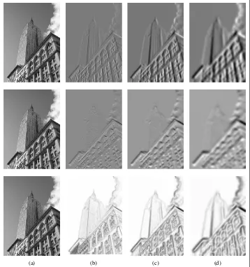
(a) (b) (c) (d)
Figure 1-11. An example of computing image derivatives using Gaussian derivatives: x-derivative (top), y-derivative (middle), and gradient magnitude (bottom); (a) original image in grayscale, (b) Gaussian derivative filter withσ=2, (c) withσ=5, (d) withσ=10.
for the details. Figure 1-11 shows the derivatives and gradient magnitude for different scales. Compare this to the blurring at the same scales in Figure 1-9.
Morphology—Counting Objects
image in which each pixel takes only two values, usually 0 and 1. Binary images are often the result of thresholding an image, for example with the intention of counting objects or measuring their size. A good summary of morphology and how it works is inhttp://en.wikipedia.org/wiki/Mathematical_morphology.
Morphological operations are included in the scipy.ndimage module morphology. Counting and measurement functions for binary images are in thescipy.ndimage mod-ulemeasurements. Let’s look at a simple example of how to use them.
Consider the binary image in Figure 1-12a.3Counting the objects in that image can be done using:
from scipy.ndimage import measurements,morphology
# load image and threshold to make sure it is binary
im = array(Image.open('houses.png').convert('L')) im = 1*(im<128)
labels, nbr_objects = measurements.label(im) print "Number of objects:", nbr_objects
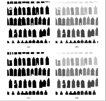
This loads the image and makes sure it is binary by thresholding. Multiplying by 1 con-verts the boolean array to a binary one. Then the functionlabel()finds the individual objects and assigns integer labels to pixels according to which object they belong to. Figure 1-12b shows thelabelsarray. The graylevel values indicate object index. As you can see, there are small connections between some of the objects. Using an operation called binary opening, we can remove them:
# morphology - opening to separate objects better
im_open = morphology.binary_opening(im,ones((9,5)),iterations=2)
labels_open, nbr_objects_open = measurements.label(im_open) print "Number of objects:", nbr_objects_open
The second argument ofbinary_opening()specifies thestructuring element, an array that indicates what neighbors to use when centered around a pixel. In this case, we used 9 pixels (4 above, the pixel itself, and 4 below) in the y direction and 5 in the x direction. You can specify any array as structuring element; the non-zero elements will determine the neighbors. The parameteriterationsdetermines how many times to apply the operation. Try this and see how the number of objects changes. The image after opening and the corresponding label image are shown in Figure 1-12c–d. As you might expect, there is a function namedbinary_closing()that does the reverse. We leave that and the other functions inmorphologyandmeasurementsto the exercises. You can learn more about them from thescipy.ndimagedocumentationhttp://docs.scipy.org/ doc/scipy/reference/ndimage.html.
3This image is actually the result of image “segmentation.” Take a look at Section 9.3 if you want to see how
this image was created.
(a) (b)
(c) (d)
Figure 1-12. An example of morphology. Binary opening to separate objects followed by counting them: (a) original binary image; (b) label image corresponding to the original, grayvalues indicate object index; (c) binary image after opening; (d) label image corresponding to the opened image.
Useful SciPy Modules
SciPy comes with some useful modules for input and output. Two of them are io
andmisc.
Reading and writing .mat files
If you have some data, or find some interesting data set online, stored in Matlab’s.mat
file format, it is possible to read this using thescipy.iomodule. This is how to do it: data = scipy.io.loadmat('test.mat')
files is equally simple. Just create a dictionary with all variables you want to save and usesavemat():
data = {} data['x'] = x
scipy.io.savemat('test.mat',data)
This saves the array x so that it has the name “x” when read into Matlab. More information onscipy.iocan be found in the online documentation,http://docs.scipy .org/doc/scipy/reference/io.html.
Saving arrays as images
Since we are manipulating images and doing computations using array objects, it is useful to be able to save them directly as image files.4Many images in this book are created just like this.
Theimsave()function is available through thescipy.miscmodule. To save an arrayim
to file just do the following: from scipy.misc import imsave imsave('test.jpg',im)
Thescipy.miscmodule also contains the famous “Lena” test image: lena = scipy.misc.lena()
This will give you a 512×512 grayscale array version of the image.
1.5 Advanced Example: Image De-Noising
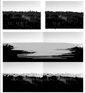
We conclude this chapter with a very useful example, de-noising of images. Image de-noisingis the process of removing image noise while at the same time trying to preserve details and structures. We will use theRudin-Osher-Fatemi de-noising model (ROF) originally introduced in [28]. Removing noise from images is important for many applications, from making your holiday photos look better to improving the quality of satellite images. The ROF model has the interesting property that it finds a smoother version of the image while preserving edges and structures.
The underlying mathematics of the ROF model and the solution techniques are quite advanced and outside the scope of this book. We’ll give a brief, simplified introduction before showing how to implement a ROF solver based on an algorithm by Cham-bolle [5].
Thetotal variation(TV) of a (grayscale) imageI is defined as the sum of the gradient norm. In a continuous representation, this is
J (I )=
|∇I|dx. (1.1)
4AllPyLabfigures can be saved in a multitude of image formats by clicking the “save” button in the figure
window.
In a discrete setting, the total variation becomes J (I )=
x
|∇I|,
where the sum is taken over all image coordinatesx=[x,y].
In the Chambolle version of ROF, the goal is to find a de-noised imageUthat minimizes min
U ||I −U||
2+2λJ (U ),
where the norm||I −U||measures the difference betweenU and the original image I. What this means is, in essence, that the model looks for images that are “flat” but allows “jumps” at edges between regions.
Following the recipe in the paper, here’s the code: from numpy import *
def denoise(im,U_init,tolerance=0.1,tau=0.125,tv_weight=100):
""" An implementation of the Rudin-Osher-Fatemi (ROF) denoising model using the numerical procedure presented in eq (11) A. Chambolle (2005). Input: noisy input image (grayscale), initial guess for U, weight of the TV-regularizing term, steplength, tolerance for stop criterion. Output: denoised and detextured image, texture residual. """
m,n = im.shape# size of noisy image # initialize
U = U_init
Px = im # x-component to the dual field
Py = im # y-component of the dual field
error = 1
while (error > tolerance): Uold = U
# gradient of primal variable
GradUx = roll(U,-1,axis=1)-U # x-component of U's gradient
GradUy = roll(U,-1,axis=0)-U # y-component of U's gradient # update the dual varible
PxNew = Px + (tau/tv_weight)*GradUx PyNew = Py + (tau/tv_weight)*GradUy
NormNew = maximum(1,sqrt(PxNew**2+PyNew**2))
Px = PxNew/NormNew# update of x-component (dual)
Py = PyNew/NormNew# update of y-component (dual) # update the primal variable
RxPx = roll(Px,1,axis=1) # right x-translation of x-component
RyPy = roll(Py,1,axis=0) # right y-translation of y-component
U = im + tv_weight*DivP # update of the primal variable # update of error
error = linalg.norm(U-Uold)/sqrt(n*m);
return U,im-U# denoised image and texture residual
In this example, we used the functionroll(), which, as the name suggests, “rolls” the values of an array cyclically around an axis. This is very convenient for computing neighbor differences, in this case for derivatives. We also usedlinalg.norm(), which measures the difference between two arrays (in this case, the image matricesU and
Uold). Save the functiondenoise()in a filerof.py. Let’s start with a synthetic example of a noisy image:
from numpy import * from numpy import random
from scipy.ndimage import filters import rof
# create synthetic image with noise
im = zeros((500,500)) im[100:400,100:400] = 128 im[200:300,200:300] = 255
im = im + 30*random.standard_normal((500,500))
U,T = rof.denoise(im,im)
G = filters.gaussian_filter(im,10)
# save the result
from scipy.misc import imsave imsave('synth_rof.pdf',U) imsave('synth_gaussian.pdf',G)
The resulting images are shown in Figure 1-13 together with the original. As you can see, the ROF version preserves the edges nicely.
(a) (b) (c)
Figure 1-13. An example of ROF de-noising of a synthetic example: (a) original noisy image; (b) image after Gaussian blurring (σ=10); (c) image after ROF de-noising.
(a) (b) (c)
Figure 1-14. An example of ROF de-noising of a grayscale image: (a) original image; (b) image after Gaussian blurring (σ=5); (c) image after ROF de-noising.
Now, let’s see what happens with a real image: from PIL import Image
from pylab import * import rof
im = array(Image.open('empire.jpg').convert('L')) U,T = rof.denoise(im,im)
figure() gray() imshow(U) axis('equal') axis('off') show()
The result should look something like Figure 1-14c, which also shows a blurred version of the same image for comparison. As you can see, ROF de-noising preserves edges and image structures while at the same time blurring out the “noise.”
Exercises
1. Take an image and apply Gaussian blur like in Figure 1-9. Plot the image contours for increasing values ofσ. What happens? Can you explain why?
3. An alternative image normalization to histogram equalization is aquotient image. A quotient image is obtained by dividing the image with a blurred versionI /(I∗Gσ).
Implement this and try it on some sample images.
4. Write a function that finds the outline of simple objects in images (for example, a square against white background) using image gradients.
5. Use gradient direction and magnitude to detect lines in an image. Estimate the extent of the lines and their parameters. Plot the lines overlaid on the image. 6. Apply thelabel()function to a thresholded image of your choice. Use histograms
and the resulting label image to plot the distribution of object sizes in the image. 7. Experiment with successive morphological operations on a thresholded image of
your choice. When you have found some settings that produce good results, try the functioncenter_of_massinmorphologyto find the center coordinates of each object and plot them in the image.
Conventions for the Code Examples
From Chapter 2 and onward, we assume PIL,NumPy, andMatplotlibare included at the top of every file you create and in every code example as:
from PIL import Image from numpy import * from pylab import *
This makes the example code cleaner and the presentation easier to follow. In the cases when we useSciPymodules, we will explicitly declare that in the examples.
Purists will object to this type of blanket imports and insist on something like import numpy as np
import matplotlib.pyplot as plt
so that namespaces can be kept (to know where each function comes from) and only import thepyplotpart ofMatplotlib, since theNumPyparts imported withPyLabare not needed. Purists and experienced programmers know the difference and can choose whichever option they prefer. In the interest of making the content and examples in this book easily accessible to readers, I have chosen not to do this.
Caveat emptor.
CHAPTER 2
Local Image Descriptors
This chapter is about finding corresponding points and regions between images. Two different types of local descriptors are introduced with methods for matching these between images. These local features will be used in many different contexts throughout this book and are an important building block in many applications, such as creating panoramas, augmented reality, and computing 3D reconstructions.
2.1 Harris Corner Detector
The Harris corner detection algorithm (or sometimes the Harris & Stephens corner detector) is one of the simplest corner indicators available. The general idea is to locate interest points where the surrounding neighborhood shows edges in more than one direction; these are then image corners.
We define a matrixMI=MI(x), on the pointsxin the image domain, as the positive
semi-definite, symmetric matrix
MI= ∇I ∇IT =
Ix
Iy
[Ix Iy]=
Ix2 IxIy
IxIy Iy2
, (2.1)
whereas before∇Iis the image gradient containing the derivativesIxandIy(we defined
the derivatives and the gradient on page 18). Because of this construction,MIhas rank
one with eigenvaluesλ1= |∇I|2andλ2=0. We now have one matrix for each pixel in the image.
Let W be a weight matrix (typically a Gaussian filter Gσ). The component-wise
convolution
MI=W ∗MI (2.2)
gives a local averaging ofMI over the neighboring pixels. The resulting matrix MI
is sometimes called aHarris matrix. The width ofW determines a region of interest around x. The idea of averaging the matrix MI over a region like this is that the
eigenvalues will change depending on the local image properties. If the gradients vary
in the region, the second eigenvalue ofMIwill no longer be zero. If the gradients are
the same, the eigenvalues will be the same as forMI.
Depending on the values of∇I in the region, there are three cases for the eigenvalues of the Harris matrix,MI:
. Ifλ
1andλ2are both large positive values, then there is a corner atx.
. Ifλ
1is large andλ2≈0, then there is an edge and the averaging ofMI over the
region doesn’t change the eigenvalues that much.
. Ifλ
1≈λ2≈0, then there is nothing.
To distinguish the important case from the others without actually having to compute the eigenvalues, Harris and Stephens [12] introduced an indicator function
det(MI)−κtrace(MI)2.
To get rid of the weighting constantκ, it is often easier to use the quotient det(MI)
trace(MI)2
as an indicator.
Let’s see what this looks like in code. For this, we need the scipy.ndimage.filters
module for computing derivatives using Gaussian derivative filters as described on page 18. The reason is again that we would like to suppress noise sensitivity in the corner detection process.
First, add the corner response function to a fileharris.py, which will make use of the Gaussian derivatives. Again, the parameterσ defines the scale of the Gaussian filters used. You can also modify this function to take different scales in thexandydirections, as well as a different scale for the averaging, to compute the Harris matrix.
from scipy.ndimage import filters
def compute_harris_response(im,sigma=3):
""" Compute the Harris corner detector response function for each pixel in a graylevel image. """
# derivatives
imx = zeros(im.shape)
filters.gaussian_filter(im, (sigma,sigma), (0,1), imx) imy = zeros(im.shape)
filters.gaussian_filter(im, (sigma,sigma), (1,0), imy)
# compute components of the Harris matrix
Wxx = filters.gaussian_filter(imx*imx,sigma) Wxy = filters.gaussian_filter(imx*imy,sigma) Wyy = filters.gaussian_filter(imy*imy,sigma)
# determinant and trace
Wdet = Wxx*Wyy - Wxy**2 Wtr = Wxx + Wyy
This gives an image with each pixel containing the value of the Harris response func-tion. Now, it is just a matter of picking out the information needed from this image. Taking all points with values above a threshold, with the additional constraint that cor-ners must be separated with a minimum distance, is an approach that often gives good results. To do this, take all candidate pixels, sort them in descending order of corner response values, and mark off regions too close to positions already marked as corners. Add the following function toharris.py:
def get_harris_points(harrisim,min_dist=10,threshold=0.1):
""" Return corners from a Harris response image min_dist is the minimum number of pixels separating corners and image boundary. """
# find top corner candidates above a threshold
corner_threshold = harrisim.max() * threshold harrisim_t = (harrisim > corner_threshold) * 1
# get coordinates of candidates
coords = array(harrisim_t.nonzero()).T
# ...and their values
candidate_values = [harrisim[c[0],c[1]] for c in coords]
# sort candidates
index = argsort(candidate_values)
# store allowed point locations in array
allowed_locations = zeros(harrisim.shape)
allowed_locations[min_dist:-min_dist,min_dist:-min_dist] = 1
# select the best points taking min_distance into account
filtered_coords = [] for i in index:
if allowed_locations[coords[i,0],coords[i,1]] == 1: filtered_coords.append(coords[i])
allowed_locations[(coords[i,0]-min_dist):(coords[i,0]+min_dist), (coords[i,1]-min_dist):(coords[i,1]+min_dist)] = 0
return filtered_coords
Now you have all you need to detect corner points in images. To show the corner points in the image, you can add a plotting function toharris.pyusingMatplotlibas follows:
def plot_harris_points(image,filtered_coords):
""" Plots corners found in image. """
figure() gray() imshow(image)
plot([p[1] for p in filtered_coords],[p[0] for p in filtered_coords],'*') axis('off')
show()