Symbolic Data Analysis and the
SODAS Software
Edited by
Edwin Diday
Université de Paris IX - Dauphine, France
Symbolic Data Analysis and the
SODAS Software
Edited by
Edwin Diday
Université de Paris IX - Dauphine, France
Telephone +441243 779777
Email (for orders and customer service enquiries): [email protected] Visit our Home Page on www.wiley.com
All Rights Reserved. No part of this publication may be reproduced, stored in a retrieval system or transmitted in any form or by any means, electronic, mechanical, photocopying, recording, scanning or otherwise, except under the terms of the Copyright, Designs and Patents Act 1988 or under the terms of a licence issued by the Copyright Licensing Agency Ltd, 90 Tottenham Court Road, London W1T 4LP, UK, without the permission in writing of the Publisher. Requests to the Publisher should be addressed to the Permissions Department, John Wiley & Sons Ltd, The Atrium, Southern Gate, Chichester, West Sussex PO19 8SQ, England, or emailed to [email protected], or faxed to (+44) 1243 770620.
This publication is designed to provide accurate and authoritative information in regard to the subject matter covered. It is sold on the understanding that the Publisher is not engaged in rendering professional services. If professional advice or other expert assistance is required, the services of a competent professional should be sought.
Other Wiley Editorial Offices
John Wiley & Sons Inc., 111 River Street, Hoboken, NJ 07030, USA
Jossey-Bass, 989 Market Street, San Francisco, CA 94103-1741, USA
Wiley-VCH Verlag GmbH, Boschstr. 12, D-69469 Weinheim, Germany
John Wiley & Sons Australia Ltd, 42 McDougall Street, Milton, Queensland 4064, Australia
John Wiley & Sons (Asia) Pte Ltd, 2 Clementi Loop #02-01, Jin Xing Distripark, Singapore 129809
John Wiley & Sons Canada Ltd, 6045 Freemont Blvd, Mississauga, ONT, L5R 4J3
Wiley also publishes its books in a variety of electronic formats. Some content that appears in print may not be available in electronic books.
Library of Congress Cataloging in Publication Data
Symbolic data analysis and the SODAS software / edited by Edwin Diday, Monique Noirhomme-Fraiture.
p. cm.
Includes bibliographical references and index. ISBN 978-0-470-01883-5 (cloth)
1. Data mining. I. Diday, E. II. Noirhomme-Fraiture, Monique. QA76.9.D343S933 2008
005.74—dc22
2007045552
British Library Cataloguing in Publication Data
A catalogue record for this book is available from the British Library
ISBN 978-0-470-01883-5
Contents
Contributors ix
Foreword xiii
Preface xv
ASSO Partners xvii
Introduction
1
1 The state of the art in symbolic data analysis: overview
and future 3
Edwin Diday
Part I
Databases versus Symbolic Objects
43
2 Improved generation of symbolic objects from relational
databases 45
Yves Lechevallier, Aicha El Golli and George Hébrail
3 Exporting symbolic objects to databases 61
Donato Malerba, Floriana Esposito and Annalisa Appice
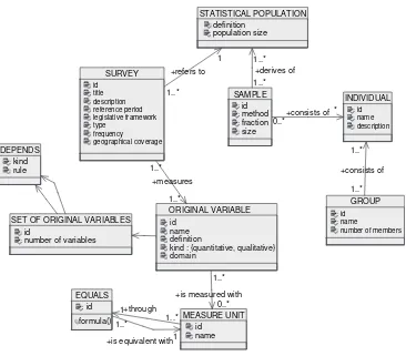
4 A statistical metadata model for symbolic objects 67
Haralambos Papageorgiou and Maria Vardaki
5 Editing symbolic data 81
Monique Noirhomme-Fraiture, Paula Brito,
Anne de Baenst-Vandenbroucke and Adolphe Nahimana
6 The normal symbolic form 93
Marc Csernel and Francisco de A.T. de Carvalho
7 Visualization 109
Part II
Unsupervised Methods
121
8 Dissimilarity and matching 123
Floriana Esposito, Donato Malerba and Annalisa Appice
9 Unsupervised divisive classification 149
Jean-Paul Rasson, Jean-Yves Pirçon, Pascale Lallemand and Séverine Adans
10 Hierarchical and pyramidal clustering 157
Paula Brito and Francisco de A.T. de Carvalho
11 Clustering methods in symbolic data analysis 181
Francisco de A.T. de Carvalho, Yves Lechevallier and Rosanna Verde
12 Visualizing symbolic data by Kohonen maps 205
Hans-Hermann Bock
13 Validation of clustering structure: determination of the
number of clusters 235
André Hardy
14 Stability measures for assessing a partition and its clusters:
application to symbolic data sets 263
Patrice Bertrand and Ghazi Bel Mufti
15 Principal component analysis of symbolic data described by
intervals 279
N. Carlo Lauro, Rosanna Verde and Antonio Irpino
16 Generalized canonical analysis 313
N. Carlo Lauro, Rosanna Verde and Antonio Irpino
Part III
Supervised Methods
331
17 Bayesian decision trees 333
Jean-Paul Rasson, Pascale Lallemand and Séverine Adans
18 Factor discriminant analysis 341
N. Carlo Lauro, Rosanna Verde and Antonio Irpino
19 Symbolic linear regression methodology 359
Filipe Afonso, Lynne Billard, Edwin Diday and Mehdi Limam
20 Multi-layer perceptrons and symbolic data 373
CONTENTS vii
Part IV
Applications and the SODAS Software
393
21 Application to the Finnish, Spanish and Portuguese data of the
European Social Survey 395
Soile Mustjärvi and Seppo Laaksonen
22 People’s life values and trust components in Europe: symbolic data
analysis for 20–22 countries 405
Seppo Laaksonen
23 Symbolic analysis of the Time Use Survey in the Basque country 421
Marta Mas and Haritz Olaeta
24 SODAS2 software: Overview and methodology 429
Anne de Baenst-Vandenbroucke and Yves Lechevallier
Contributors
Séverine Adans, Facultés Universitaires Notre-Dame de la Paix, Déprt. de Mathematique, Rempart de la Vierge, 8, Namur, Belgium, B-5000
Filipe Afonso, Université Paris IX-Dauphine, LISE-CEREMADE, Place du Maréchal de Lattre de Tassigny, Paris Cedex 16, France, F-75775
Annalisa Appice, Floriana Esposito Universita degli Studi di Bari, Dipartimento di Infor-matica, v. Orabona, 4, Bari, Italy, I-70125
Anne de Baenst-Vandenbroucke, Facultés Universitaires Notre-Dame de la Paix, Faculté d’Informatique, Rue Grandgagnage, 21, Namur, Belgium, B-5000, [email protected]
Ghazi Bel Mufti, ESSEC de Tunis, 4 rue Abou Zakaria El Hafsi, Montfleury 1089, Tunis, Tunisia, [email protected]
Patrice Bertrand, Ceremade, Université Paris IX-Dauphine, Place du Maréchal de Lattre de Tassigny, Paris Cedex 16, France, F-75775, [email protected]
Lynne Billard, University of Georgia, Athens, USA, GA 30602-1952, [email protected]
Hans-Hermann Bock, Rheinisch-Westfälische Technische Hochschule Aachen, Institut für Statistik und Wirtschaftmathematik, Wüllnerstr. 3, Aachen, Germany, D-52056, [email protected]
Maria Paula de Pinho de Brito, Faculdade de Economia do Porto, LIACC, Rua Dr. Roberto Frias, Porto, Portugal, P-4200-464, [email protected]
Brieuc Conan-Guez, LITA EA3097, Université de Metz, Ile de Saulcy, F-57045, Metz, France, [email protected]
Francisco de A.T. de Carvalho, Universade Federale de Pernambuco, Centro de Infor-matica, Av. Prof. Luis Freire s/n - Citade Universitaria, Recife-PE, Brasil, 50740-540, [email protected]
Edwin Diday, Université Paris IX-Dauphine, LISE-CEREMADE, Place du Marechal de Lattre de Tassigny, Paris Cedex 16, France F-75775, [email protected]
Aicha El Golli, INRIA Paris, Unité de Recherche de Roquencourt, Domaine de Voluceau, BP 105, Le Chesnay Cedex, France, F-78153, [email protected]
Floriana Esposito, Universita degli Studi di Bari, Dipartimento di Informatica, v. Orabona, 4, Bari, Italy, I-70125, [email protected]
André Hardy, Facultés Universitaires Notre-Dame de la Paix, Départment de Mathématique, Rempart de la Vièrge, 8, Namur, Belgium, B-5000, [email protected]
Georges Hébrail, Laboratoire LTCI UMR 5141, Ecole Nationale Supériewe des Télécom-munications, 46 rue Barrault, 75013 Paris, France, [email protected]
Antonio Irpino, Universita Frederico II, Dipartimento di Mathematica e Statistica, Via Cinthia, Monte Sant’Angelo, Napoli, Italy I-80126, [email protected]
Seppo Laaksonen, Statistics Finland, Box 68, University of Helsinki, Finland, FIN 00014, [email protected]
Pascale Lallemand, Facultés Universitaires Notre-Dame de la Paix, Départment de Mathé-matique, Rempart de la Vièrge, 8, Namur, Belgium, B-5000
Natale Carlo Lauro, Universita Frederico II, Dipartimento di Mathematica e Statistica, Via Cinthia, Monte Sant’Angelo, Napoli, Italy I-80126, [email protected]
Yves Lechevallier, INRIA, Unité de Recherche de Roquencourt, Domaine de Voluceau, BP 105, Le Chesnay Cedex, France, F-78153, Yves. [email protected]
Mehdi Limam, Université Paris IX-Dauphine, LISE-CEREMADE, Place du Maréchal de Lattre de Tassigny, Paris Cedex 16, France, F-75775
Donato Malerba, Universita degli Studi di Bari, Dipartimento di Informatica, v. Orabona, 4, Bari, Italy, I-70125, [email protected]
Marta Mas, Asistencia Tecnica y Metodologica, Beato Tom´ as de Zumarraga, 52, 3´ -Izda, Vitoria-Gasteiz, Spain, E-01009, [email protected]
CONTRIBUTORS xi
Adolphe Nahimana, Facultés Universitaires Notre-Dame de la Paix, Faculté d’Informatique, Rue Grandgagnage, 21, Namur, Belgium, B-5000
Monique Noirhomme-Fraiture, Facultés Universitaires Notre-Dame de la Paix, Faculté d’Informatique, Rue Grandgagnage, 21, Namur, Belgium, B-5000, [email protected]
Haritz Olaeta, Euskal Estatistika Erakundea, Area de Metodologia, Donostia, 1, Vitoria-Gasteiz, Spain, E-010010, [email protected]
Haralambos Papageorgiou, University of Athens, Department of Mathematics, Panepis-temiopolis, Athens, Greece, EL-15784, [email protected]
Jean-Yves Pirçon, Facultés Universitaires Notre-Dame de la Paix, Déprt. de Mathematique, Rempart de la Vièrge, 8, Namur, Belgium, B-5000
Jean-Paul Rasson, Facultés Universitaires Notre-Dame de la Paix, Départ. de Mathematique, Rempart de la Vièrge, 8, Namur, Belgium, B-5000, [email protected]
Fabrice Rossi, Projet AxIS, INRIA, Centre de Rechoche Paris-Roquencourt, Domaine de Volucean, BP 105, Le Chesney Cedex, France F-78153, [email protected]
Maria Vardaki, University of Athens, Department of Mathematics, Panepistemiopolis, Athens, Greece, EL-15784 [email protected]
Foreword
It is a great pleasure for me to preface this imposing work which establishes, withAnalysis of Symbolic Data(Bock and Diday, 2000) andSymbolic Data Analysis(Billard and Diday,
2006), a true bible as well as a practical handbook.
Since the pioneering work of Diday at the end of the 1980s, symbolic data analysis has spread beyond a restricted circle of researchers to attain a stature attested to by many publications and conferences. Projects have been supported by Eurostat (the statistical office of the European Union), and this recognition of symbolic data analysis as a tool for official statistics was also a crucial step forward.
Symbolic data analysis is part of the great movement of interaction between statistics and data processing. In the 1960s, under the impetus of J. Tukey and of J.P. Benzécri, exploratory data analysis was made possible by progress in computation and by the need to process the data which one stored. During this time, large data sets were tables of a few thousand units described by a few tens of variables. The goal was to have the data speak directly without using overly simplified models. With the development of relational databases and data warehouses, the problem changed dimension, and one might say that it gave birth on the one hand to data mining and on the other hand to symbolic data analysis. However, this convenient opposition or distinction is somewhat artificial.
Data mining and machine learning techniques look for patterns (exploratory or unsuper-vised) and models (superunsuper-vised) by processing almost all the available data: the statistical unit remains unchanged and the concept of model takes on a very special meaning. A model is no longer a parsimonious representation of reality resulting from a physical, biological, or economic theory being put in the form of a simple relation between variables, but a fore-casting algorithm (often a black box) whose quality is measured by its ability to generalize to new data (which must follow the same distribution). Statistical learning theory provides the theoretical framework for these methods, but the data remain traditional data, represented in the form of a rectangular table of variables and individuals where each cell is a value of a numeric variable or a category of a qualitative variable assumed to be measured without error.
data analysis can be considered as the statistical theory associated with relational databases. It is not surprising that symbolic data analysis found an important field of application in official statistics where it is essential to present data at a high level of aggregation rather than to reason on individual data. For that, a rigorous mathematical framework has been developed which is presented in a comprehensive way in the important introductory chapter of this book.
Once this framework was set, it was necessary to adapt the traditional methods to this new type of data, and Parts II and III show how to do this both in exploratory analysis (including very sophisticated methods such as generalized canonical analysis) and in supervised analysis where the problem is the interrelation and prediction of symbolic variables. The chapters dedicated to cluster analysis are of great importance. The methods and developments gathered together in this book are impressive and show well that symbolic data analysis has reached full maturity.
In an earlier paragraph I spoke of the artificial opposition of data mining and symbolic data analysis. One will find in this book symbolic generalizations of methods which are typical of data mining such as association rules, neural networks, Kohonen maps, and classification trees. The border between the two fields is thus fairly fluid.
What is the use of sound statistical methods if users do not have application software at their disposal? It is one of the strengths of the team which contributed to this book that they have also developed the freely available software SODAS2. I strongly advise the reader to use SODAS2 at the same time as he reads this book. One can only congratulate the editors and the authors who have brought together in this work such an accumulation of knowledge in a homogeneous and accessible language. This book will mark a milestone in the history of data analysis.
Preface
This book is a result of the European ASSO project (IST-2000-25161) http://www. assoproject.be on an Analysis System of Symbolic Official data, within the Fifth Framework Programme. Some 10 research teams, three national institutes for statistics and two private companies have cooperated in this project. The project began in January 2001 and ended in December 2003. It was the follow-up to a first SODAS project, also financed by the European Community.
The aim of the ASSO project was to design methods, methodology and software tools for extracting knowledge from multidimensional complex data (www.assoproject.be). As a result of the project, new symbolic data analysis methods were produced and new software, SODAS2, was designed. In this book, the methods are described, with instructive examples, making the book a good basis for getting to grips with the methods used in the SODAS2 software, complementing the tutorial and help guide. The software and methods highlight the crossover between statistics and computer science, with a particular emphasis on data mining.
The book is aimed at practitioners of symbolic data analysis – statisticians and economists within the public (e.g. national statistics institutes) and private sectors. It will also be of interest to postgraduate students and researchers within data mining.
Acknowledgements
The editors are grateful to ASSO partners and external authors for their careful work and contributions. All authors were asked to review chapters written by colleagues so that we could benefit from internal cross-validation. In this regard, we wish especially to thank Paula Brito, who revised most of the chapters. Her help was invaluable. We also thank Pierre Cazes who offered much substantive advice. Thanks are due to Photis Nanopulos and Daniel Defays of the European Commission who encouraged us in this project and also to our project officer, Knut Utwik, for his patience during this creative period.
ASSO Partners
FUNDP Facultés Universitaires Notre-Dame de la Paix, Institut d’Informatique, Rue Grandgagnage, 21, Namur, Belgium, B-5000 [email protected] (coordinator)
DAUPHINE Université Paris IX-Dauphine, LISE-CEREMADE, Place du Maréchal de Lattre de Tassigny, Paris Cedex 16, France, F-75775 [email protected]
DIB Universita degli Studi di Bari, Dipartimento di Informatica, v. Orabona, 4, Bari, Italy, I-70125 [email protected]
DMS Dipartimento di Mathematica e Statistica, Via Cinthia, Monte Sant’Angelo, Napoli, Italy I-80126 [email protected]
EUSTAT Euskal Estatistika Erakundea, Area de Metodologia, Donostia, 1, Vitoria-Gasteiz, Spain, E-01010 [email protected]
FEP Faculdade de Economia do Porto, LIACC, Rua Dr. Roberto Frias, Porto, Portugal, P-4200-464 [email protected]
FUNDPMa Facultés Universitaires Notre-Dame de la Paix, Rempart de la Vierge, 8, Namur, Belgium, B-5000 [email protected]
INRIA, Unité de Recherche de Roquencourt, Domaine de Voluceau, BP 105, Le Chesnay Cedex, France, F-78153 [email protected]
INS Instituto Nacional de Estatistica, Direcçao Regional de Lisboa e Valo do Tejo, Av. Antonio José de Almeida, Lisboa, Portugal, P-1000-043 [email protected]
SPAD Groupe TestAndGO, Rue des petites Ecuries, Paris, France, F-75010 [email protected]
STATFI Statistics Finland, Management Services/R&D Department, Tyoepajakatu, 13, Statistics Finland, Finland, FIN-00022 [email protected]
TES Institute ASBL, Rue des Bruyères, 3, Howald, Luxembourg, L-1274
UFPE Universade Federale de Pernambuco, Centro de Informatica-Cin, Citade Universi-taria, Recife-PE, Brasil, 50740-540 [email protected]
1
The state of the art in symbolic
data analysis: overview
and future
Edwin Diday
1.1 Introduction
Databases are now ubiquitous in industrial companies and public administrations, and they often grow to an enormous size. They contain units described by variables that are often categorical or numerical (the latter can of course be also transformed into categories). It is then easy to construct categories and their Cartesian product. In symbolic data analysis these categories are considered to be the new statistical units, and the first step is to get these higher-level units and to describe them by taking care of their internal variation. What do we mean by ‘internal variation’? For example, the age of a player in a football team is 32 but the age of the players in the team (considered as a category) varies between 22 and 34; the height of the mushroom that I have in my hand is 9 cm but the height of the species (considered as a category) varies between 8 and 15 cm.
A more general example is a clustering process applied to a huge database in order to summarize it. Each cluster obtained can be considered as a category, and therefore each variable value will vary inside each category. Symbolic data represented by structured variables, lists, intervals, distributions and the like, store the ‘internal variation’ of categories better than do standard data, which they generalize. ‘Complex data’ are defined as structured data, mixtures of images, sounds, text, categorical data, numerical data, etc. Therefore, symbolic data can be induced from categories of units described by complex data (see Section 1.4.1) and therefore complex data describing units can be considered as a special case of symbolic data describing higher-level units.
The aim of symbolic data analysis is to generalize data mining and statistics to higher-level units described by symbolic data. The SODAS2 software, supported by EURO-STAT, extends the standard tools of statistics and data mining to these higher-level units. More precisely, symbolic data analysis extends exploratory data analysis (Tukey, 1958; Benzécri, 1973; Didayet al., 1984; Lebartet al., 1995; Saporta, 2006), and data mining (rule
discovery, clustering, factor analysis, discrimination, decision trees, Kohonen maps, neural networks, ) from standard data to symbolic data.
Since the first papers announcing the main principles of symbolic data analysis (Diday, 1987a, 1987b, 1989, 1991), much work has been done, up to and including the publication of the collection edited by Bock and Diday (2000) and the book by Billard and Diday (2006). Several papers offering a synthesis of the subject can be mentioned, among them Diday (2000a, 2002a, 2005), Billard and Diday (2003) and Diday and Esposito (2003). The symbolic data analysis framework extends standard statistics and data mining tools to higher-level units and symbolic data. For example, standard descriptive statistics (mean, variance, correlation, distribution, histograms, ) are extended in de Carvalho (1995),
Bertrand and Goupil (2000), Billard and Diday (2003, 2006), Billard (2004) and Gioia and Lauro (2006a). Standard tools of multidimensional data analysis such as principal component analysis are extended in Cazes et al. (1997), Lauro et al. (2000), Irpino et al.
(2003), Irpino (2006) and Gioia and Lauro (2006b). Extensions of dissimilarities to symbolic data can be found in Bock and Diday (2000, Chapter 8), in a series of papers by Esposito
et al. (1991, 1992) and also in Malerbaet al. (2002), Diday and Esposito (2003) and Bock
(2005). On clustering, recent work by de Souza and de Carvalho (2004), Bock (2005), Diday and Murty (2005) and de Carvalho et al. (2006a, 2006b) can be mentioned. The
problem of the determination of the optimum number of clusters in clustering of symbolic data has been analysed by Hardy and Lallemand (2001, 2002, 2004), Hardy et al. (2002)
and Hardy (2004, 2005). On decision trees, there are papers by Ciampiet al. (2000), Bravo
and García-Santesmases (2000), Limamet al. (2003), Bravo Llatas (2004) and Mballoet al.
(2004). On conceptual Galois lattices, we have Diday and Emilion (2003) and Brito and Polaillon (2005). On hierarchical and pyramidal clustering, there are Brito (2002) and Diday (2004). On discrimination and classification, there are papers by Duarte Silva and Brito (2006), Appiceet al. (2006). On symbolic regression, we have Afonsoet al. (2004) and de
Carvalhoet al. (2004). On mixture decomposition of vectors of distributions, papers include
Diday and Vrac (2005) and Cuvelier and Noirhomme-Fraiture (2005). On rule extraction, there is the Afonso and Diday (2005) paper. On visualization of symbolic data, we have Noirhomme-Fraiture (2002) and Irpinoet al. (2003). Finally, we might mention Prudêncio et al. (2004) on time series, Souleet al. (2004) on flow classification, Vracet al. (2004) on
meteorology, Caruso et al. (2005) on network traffic, Bezera and de Carvalho (2004) on
information filtering, and Da Silvaet al. (2006) and Meneses and Rodríguez-Rojas (2006)
on web mining.
FROM STANDARD DATA TABLES TO SYMBOLIC DATA TABLES 5
kinds of variable (numerical, categorical, interval, categorical multi-valued, modal), the conceptual variables which describe concepts and the background knowledge by means of taxonomies and rules. Section 1.4 provides some general applications of the symbolic data analysis paradigm. It is shown that from fuzzy or uncertainty data, symbolic descriptions are needed in order to describe classes, categories or concepts. Another application concerns the possibility of fusing data tables with different entries and different variables by using the same concepts and their symbolic description. Finally, it is shown that much information is lost if a symbolic description is transformed into a standard classical description by transforming, for example, an interval into two variables (the maximum and minimum). In Section 1.5 the main steps and principles of a symbolic data analysis are summarized. Section 1.6 provides more details on the method of modelling concepts by symbolic objects based on four spaces (individuals and concepts of the ‘real world’ and their associated symbolic descriptions and symbolic objects in the ‘modelled world’). The definition, extent and syntax of symbolic objects are given. This section ends with some advantages of the use of symbolic objects and how to improve them by means of a learning process. In Section 1.7 it is shown that a generalized kind of conceptual lattice constitutes the underlying structure of symbolic objects (readers not interested in conceptual lattices can skip this section). The chapter concludes with an overview of the chapters of the book and of the SODAS2 software.
1.2 From standard data tables to symbolic data tables
Extracting knowledge from large databases is now fundamental to decision-making. In practice, the aim is often to extract new knowledge from a database by using a standard data table where the entries are a set of units described by a finite set of categorical or quantitative variables. The aim of this book is to show that much information is lost if the units are straitjacketed by such tables and to give a new framework and new tools (implemented in SODAS2) for the extraction of complementary and useful knowledge from the same database. In contrast to the standard data table model, several levels of more or less general units have to be considered as input in any knowledge extraction process. Suppose we have a standard data table giving the species, flight ability and size of 600 birds observed on an island (Table 1.1). Now, if the new units are the species of birds on the island (which are an example of what are called ‘higher-level’ units), a different answer to the same questions is obtained since, for example, the number of flying birds can be different from the number of flying species. In order to illustrate this simple example with some data, Table 1.2 describes the three species of bird on the island: there are 100 ostriches, 100 penguins and 400 swallows. The frequencies for the variable ‘flying’ extracted from this table are the reverse of those extracted from Table 1.1, as shown in Figures 1.1 and 1.2. This means that the ‘micro’ (the birds) and the ‘macro’ (the species) points of view can give results which are totally different as the frequency of flying birds in the island is 2/3 but the frequency of the flying species is 1/3.
On an island there are 600 hundred birds:
400 swallows,
100 ostriches,
100 penguins
Figure 1.1 Three species of 600 birds together.
Table 1.1 Description of 600 birds by three variables.
Birds Species Flying Size
1 Penguin No 80
599 Swallow Yes 70
600 Ostrich No 125
Table 1.2 Description of the three species of birds plus
the conceptual variable ‘migration’.
Species Flying Size Migration
Swallow {Yes} [60, 85]
Ostrich {No} [85, 160]
Penguin {No} [70, 95]
Flying Not Flying Frequency of species
2/3
Flying Not Flying 1/3
Frequency of birds
1/3 2/3
Figure 1.2 Frequencies for birds (individuals) and species (concepts).
FROM STANDARD DATA TABLES TO SYMBOLIC DATA TABLES 7
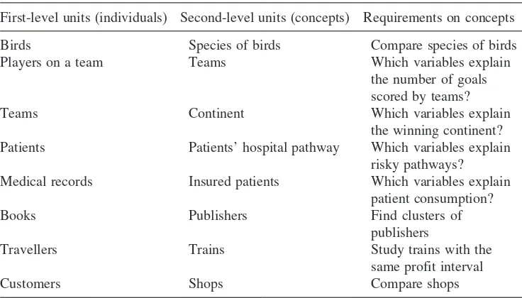
Table 1.3 Examples of first- and second-order units and requirements on the second-order
units (i.e., the concepts).
First-level units (individuals) Second-level units (concepts) Requirements on concepts
Birds Species of birds Compare species of birds
Players on a team Teams Which variables explain
the number of goals scored by teams?
Teams Continent Which variables explain
the winning continent?
Patients Patients’ hospital pathway Which variables explain
risky pathways?
Medical records Insured patients Which variables explain
patient consumption?
Books Publishers Find clusters of
publishers
Travellers Trains Study trains with the
same profit interval
Customers Shops Compare shops
Table 1.4 Initial classical data table describing players by three numerical
and two categorical variables.
Player Team Age Weight Height Nationality1
Fernández Spain 29 85 184 Spanish
Rodríguez Spain 23 90 192 Brazilian
Mballo France 25 82 190 Senegalese
Zidane France 27 78 185 French
Table 1.5 Symbolic data table obtained from Table 1.4 by describing the concepts ‘Spain’
and ‘France’.
Team AGE WEIGHT HEIGHT Nationality3 FUNDS Number of goals at
the World Cup 1998
Spain [23, 29] [85, 90] [1.84, 1.92] (0.5 Sp, 0.5 Br) 110 18
France [21, 28] [85, 90] [1.84, 1.92] (0.5 Fr, 0.5 Se) 90 24
variable denoted ‘AGE’ such that AGE(Spain) =2329. The categorical variables (such as the nationality or the place of birth) of Table 1.4 are no longer categorical in the symbolic data table. They are transformed into new variables whose values are several categories with weights defined by the frequencies of the nationalities (before naturalization in some cases), place of birth, etc., in each team. It is also possible to enhance the description of the higher-level units by adding new variables such as the variable ‘funds’ which concerns the higher-level units (i.e., the teams) and not the lower-level units (i.e., the players). Even if the teams are considered in Table 1.5 as higher-level units described by symbolic data, they can be considered as lower-level units of a higher-level unit which are the continents, in which case the continents become the units of a higher-level symbolic data table.
The concept of a hospital pathway followed by a given patient hospitalized for a disease can be defined by the type of healthcare institution at admission, the type of hospital unit and the chronological order of admission in each unit. When the patients are first-order units described by their medical variables, the pathways of the patients constitute higher-level units as several patients can have the same pathway. Many questions can be asked which concern the pathways and not the patients. For example, to compare the pathways, it may be interesting to compare their symbolic description based on the variables which describe the pathways themselves and on the medical symbolic variables describing the patients on the pathways.
Given the medical records of insured patients for a given period, the first-order units are the records described by their medical consumption (doctor, drugs, ); the second-order
units are the insured patients described by their own characteristics (age, gender, ) and
by the symbolic variables obtained from the first-order units associated with each patient. A natural question which concerns the second-order units and not the first is, for example, what explains the drug consumption of the patients? Three other examples are given in Table 1.3: when the individuals are books, each publisher is associated with a class of books; hence, it is possible to construct the symbolic description of each publisher or of the most successful publishers and compare them; when the individuals are travellers taking a train, it is possible to obtain the symbolic description of classes of travellers taking the same train and study, for example, the symbolic description of trains having the same profit interval. When the individuals are customers of shops, each shop can be associated with the symbolic description of its customers’ behaviour and compared with the other shops.
1.3 From individuals to categories, classes and concepts
1.3.1 Individuals, categories, classes, concepts
FROM INDIVIDUALS TO CATEGORIES, CLASSES AND CONCEPTS 9
intent of a concept is modelled mathematically by a generalization process applied to a set of individuals considered to belong to the extent of the concept. The following section aims to explain this process.
1.3.2 The generalization process, symbolic data and symbolic variables
A generalization process is applied to a set of individuals in order to produce a ‘symbolic description’. For example, the concept ‘swallow’ is described (see Table 1.2) by the descrip-tion vector d = ({yes}, [60, 85], [90% yes, 10% no]). The generalization process must take care of the internal variation of the description of the individuals belonging in the set of individuals that it describes. For example, the 400 swallows on the island vary in size between 60 and 85. The variable ‘colour’ could also be considered; hence, the colour of the ostriches can be white or black (which expresses a variation of the colour of the ostriches on this island between white and black), the colour of the penguins is always black and white (which does not express any variation but a conjunction valid for all the birds of this species), and the colour of the swallows is black and white or grey. This variation leads to a new kind of variable defined on the set of concepts, as the value of such variables for a concept may be a single numerical or categorical value, but also an interval, a set of ordinal or categorical values that may or may not be weighted, a distribution, etc. Since these values are not purely numerical or categorical, they have been called ‘symbolic data’. The associated variables are called ‘symbolic variables’.More generally, in order to find a unique description for a concept, the notion of the ‘T-norm of descriptive generalization’ can be used (see, for example, Diday, 2005). The T-norm operator (Schweizer and Sklar, 2005) is defined from 01×01 to [0, 1]. In order to get a symbolic descriptiondCof C(i.e., of the concept for whichCis an extent),
an extension to descriptions of the usual T-norm can be used; this is called a ‘T-norm of descriptive generalization’.
Bandemer and Nather (1992) give many examples of T-norms and T-conorms which can be generalized to T-norms and T-conorms of descriptive generalization. For example, it is easy to see that the infimum and supremum (denoted inf and sup) are respectively a T-norm and a T-coT-norm. They are also a T-T-norm and T-coT-norm of descriptive generalization. Let DC be the set of descriptions of the individuals of C. It follows that the interval
GyC=infDCsupDCconstitutes a good generalization ofDC, as its extent defined by the set of descriptions included in the interval containsC in a good and narrow way.
LetC= w1 w2 w3andDC= yw1 yw2 yw3=yC. In each of the following examples, the generalization ofCfor the variableyis denotedGyC.
1. Suppose that y is a standard numerical variable such that yw1=25 yw2=
36 yw3=71. Let D be the set of values included in the interval [1, 100]. Then
GyC=2571is the generalization ofDC for the variabley.
2. Suppose thatyis a modal variable of ordered (e.g., small, medium, large) or not ordered
(e.g., London, Paris, ) categories, such that:yw1=11/322/3(where 2(2/3) means that the frequency of the category 2 is 2/3),yw2=11/221/2 yw3= 11/423/4. Then, GyC=11/411/2 21/223/4 is the
3. Suppose that y is a variable whose values are intervals such that: yw1= 1532 yw2=364 yw3=7184. Then,GyC=1584is the
gener-alization ofDC for the variabley.
Instead of describing a class by its T-norm and T-conorm, many alternatives are possible by taking account, for instance, of the existence of outliers. A good strategy consists of reducing the size of the boundaries in order to reduce the number of outliers. This is done in DB2SO (see Chapter 2) within the SODAS2 software by using the ‘gap test’ (see Stéphan, 1998). Another choice in DB2SO is to use the frequencies in the case of categorical variables.
For example, suppose that C= w1 w2 w3, y is a standard unordered categorical variable such thatyw1=2 yw2=2 yw3=1,Dis the set of probabilities on the values 1, 2. ThenG′yC=11/322/3is the generalization ofD
C= yw1 yw2 yw3=
yCfor the variabley.
1.3.3 Inputs of a symbolic data analysis
In this book five main kinds of variables are considered: numerical (e.g., height(Tom)= 1.80); interval (e.g., age(Spain) = [23, 29]); categorical single-valued (e.g., Nationality1(Mballo)={Congo}); categorical multi-valued (e.g., Nationality2(Spain) = {Spanish, Brazilian, French}); and modal (e.g., Nationality3(Spain) = {(0.8)Spanish, (0.1)Brazilian, (0.1)French}, where there are several categories with weights).
‘Conceptual variables’ are variables which are added to the variables which describe the second-order units, because they are meaningful for the second-order units but not for the first-order units. For example, the variable ‘funds’ is a conceptual variable as it is added at the level where the second-order units are the football teams and would have less meaning at the level of the first-order units (the players). In the SODAS2 software, within the DB2SO module, the option ADDSINGLE allows conceptual variables to be added (see Chapter 2).
From lower- to higher-level units missing data diminish in number but may exist. That is why SODAS2 allows them to be taken into account(see Chapter 24). Nonsense data may also occur and can be also introduced in SODAS2 by the so-called ‘hierarchically dependent variables’ or ‘mother–daughter’ variables. For example, the variable ‘flying’ whose answer is ‘yes’ or ‘no’, has a hierarchical link with the variable ‘speed of flying’. The variable ‘flying’ can be considered as the mother variable and ‘speed of flying’ as the daughter. As a result, for a flightless bird, the variable ‘speed of flying’ is ‘not applicable’.
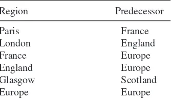
In the SODAS2 software it is also possible to add to the input symbolic data table some background knowledge, such taxonomies and some given or induced rules. For example, the variable ‘region’ can be given with more or less specificity due, for instance, to confi-dentiality. This variable describes a set of companies in Table 1.6. The links between its values are given in Figure 1.3 by a taxonomic tree and represented in Table 1.7 by two columns, associating each node of the taxonomic tree with its predecessor.
Logical dependencies can also be introduced as input; for example, ‘if age(w) is less than 2 months, then height(w) is less than 80’. As shown in the next section, these kinds of
FROM INDIVIDUALS TO CATEGORIES, CLASSES AND CONCEPTS 11
Table 1.6 Region is a taxonomic variable defined by
Table 1.7 or by Figure 1.3.
Company Region
Comp1 Paris
Comp2 London
Comp3 France
Comp4 England
Comp5 Glasgow
Comp6 Europe
Europe
United Kingdom
England Scotland France
London Glasgow Paris
Figure 1.3 Taxonomic tree associated with the variable ‘region’.
Table 1.7 Definition of the taxonomic
variable ‘region’.
Region Predecessor
Paris France
London England
France Europe
England Europe
Glasgow Scotland
Europe Europe
1.3.4 Retaining background knowledge after the generalization
process
Overgeneralization happens, for example, when a class of individuals described by a numerical variable is generalized by an interval containing smaller and greater values. For example, in Table 1.5 the age of the Spain team is described by the interval [23, 29]; this is one of several possible choices. Problems with choosing [min, max] can arise when these extreme values are in fact outliers or when the set of individuals to generalize is in fact composed of subsets of different distributions. These two cases are considered in Chapter 2. How can correlations lost by generalization be recaptured? It suffices to create new variables associated with pairs of the initial variables. For example, a new variable called Cor(yiyj) can be associated with the variablesyi andyj. Then the value of such a variable for a class of individualsCkis the correlation between the variablesyiandyjon a population reduced to the individuals of this class. For example, in Table 1.8 the players in the World Cup are described by their team, age, weight, height, nationality, etc. and by the categorical variable ‘World Cup’ which takes the value yes or no depending on the fact that they have played in or have been eliminated from the World Cup. In Table 1.9, the categories defined by the variable ‘World Cup’ constitute the new unit and the variable Cor(Weight, Height) has been added and calculated. As a result, the correlation between the weight and the height is greater for the players who play in the World Cup than for the others. In the same way, other variables can be added to the set of symbolic variables as variables representing the mean, the mean square, the median and other percentiles associated with each higher-level unit.
In the same way, it can be interesting to retain the contingency between two or more categorical variables describing a concept. This can be done simply by creating new variables which expresses this contingency. For example, if y1 is a categorical variable with four categories andy2is a variable with six categories, a new model variabley3with 24 categories which is the Cartesian product of y1 andy2 can be created for each concept. In the case of numerical variables, it is also possible to retain the number of units inside an interval or inside a product of intervals describing a concept by adding new variables expressing the number of individuals that they contain. For example, suppose that the set of birds in Table 1.1 is described by two numerical variables, ‘size’ and ‘age’, and the species swallow is described by the cross product of two confidence intervals:Iswallow(size) andIswallow(age). The extent of the concept ‘swallow’ described by the cross productIswallow (size)×Iswallow (age) among the birds can be empty or more or less dense. By keeping the contingencies information among the 600 hundred birds for each concept, a biplot representation of the
Table 1.8 Classical data table describing players by numerical and categorical variables.
Player Team Age Weight Height Nationality1 World Cup
Ferández Spain 29 85 1.84 Spanish yes
Rodríguez Spain 23 90 1.92 Brazilian yes
Mballo France 25 82 1.90 Senegalese yes
Zidane France 27 78 1.85 French yes
… … …
Renie XX 23 91 1. 75 Spanish no
Olar XX 29 84 1.84 Brazilian no
Mirce XXX 24 83 1.83 Senegalese no
GENERAL APPLICATIONS OF THE SYMBOLIC DATA ANALYSIS APPROACH 13
Table 1.9 Symbolic data table obtained from Table 1.8 by generalization
for the variables age, weight and height and keeping back the correlations between weight and height.
World Cup Age Weight Height Cov (Weight, Height)
yes [21, 26] [78, 90] [1.85, 1.98] 0.85
no [23, 30] [81, 92] [1.75, 1.85] 0.65
Table 1.10 Initial classical data table where individuals
are described by three variables.
Individuals Concepts Y1 Y2
I1 C1 a 2
I2 C1 b 1
I3 C1 c 2
I4 C2 b 1
I5 C2 b 3
I6 C2 a 2
Table 1.11 Symbolic data table induced from Table 1.10
with background knowledge defined by two rules: Y1= a⇒Y2=2andY2=1⇒Y1=b.
Y1 Y2
C1 {a,b,c} {1, 2}
C2 {a,b} {1, 2, 3}
species with these two variables will be enhanced by visualizing the density in each obtained rectangleIspecies (size)×Ispecies(age) for each species.
Finally, how can rules lost by generalization be recaptured? Rules can be induced from the initial standard data table and then added as background knowledge to the symbolic data table obtained by generalization. For example, from the simple data table in Table 1.10 two rules can be induced: Y1=a⇒Y2=2andY2=1⇒Y1=b. These rules can be added as background knowledge to the symbolic data table (Table 1.11) which describes the conceptsC1 andC2by categorical multi-valued variables.
1.4 Some general applications of the symbolic data analysis
approach
1.4.1 From complex data to symbolic data
Table 1.12 Patients described by complex data which can be transformed into classical numerical or categorical variables.
Patient Category X-Ray Radiologist text Doctor text Professional category Age
Patient1 Cj X-Ray1 Rtext1 Dtext1 Worker 25
Patientn Ck X-Rayn Rtextn Dtextn Self-employed
Table 1.13 Describing categories of patients from Table 1.12 using symbolic data.
Categories X-Ray Radiologist text Doctor text Professional category Age
C1 {X-Ray}1 {Rtext}1 {Dtext}1 {worker, unemployed} [20, 30]
Ck {X-Ray}k {Rtext}k {Dtext}k {self-employed} [35, 55]
specifically, spatial-temporal data or heterogeneous data describing, for example, a medical patient using a mixture of images, text documents and socio-demographic information. In practice, complex objects can be modelled by units described by more or less complex data. Hence, when a description of concepts, classes or categories of such complex objects is required, symbolic data can be used. Tables 1.12 and 1.13 show how symbolic data are used to describe categories of patients; the patients are the units of Table 1.12 and the categories of patients are the (higher-level) units of Table 1.13.
In Table 1.12 patients are described by their category of cancer (level of cancer, for example), an X-ray image, a radiologist text file, a doctor text file, their professional category (PC) and age. In Table 1.13, each category of cancer is described by a generalization of the X-ray image (radiologist text file, doctor text file} denoted {X-Ray} ({Rtext}, {Dtext}). When the data in Table 1.12 are transformed into standard numerical or categorical data, the resulting data table, Table 1.13, contains symbolic data obtained by the generalization process. For example, for a given category of patients, the variable PC is transformed into a histogram-valued variable by associating the frequencies of each PC category in this category of patients; the variable age is transformed to an interval variable by associating with each category the confidence interval of the ages of the patients of this category.
GENERAL APPLICATIONS OF THE SYMBOLIC DATA ANALYSIS APPROACH 15
Table 1.14 Initial data describing mushrooms of different species.
Specimen Species Stipe
thickness
Stipe length
Cap size Cap colour
Mushroom1 Amanita muscaria 15 21 24±1 red
Mushroom2 Amanita muscaria 23 15 18±1 red∧white
Mushroom3 Amanita phalloides 12 10 7±05 olive green
Mushroom4 Amanita phalloides 20 19 15±1 olive brown
Stipe thickness
0.5
1 Small Average Large
0.8
0 1.6 2.4
1.2
Membership value
2.3 1.5 2.0
Figure 1.4 From numerical data to fuzzy data: if the stipe thickness is 1.2, then it is (0.5)
Small, (0.5) Average, (0) High.
‘Imprecise data’ are obtained when it is not possible to get an exact measure. For example, it is possible to say that the height of a tree is 10 metres±1. This means that its length varies in the interval [9, 11].
‘Conjunctive data’ designate the case where several categories appear simultaneously. For example, the colour of an apple can be red or green or yellow but it can be also ‘red and yellow’.
When individuals are described by fuzzy and/or imprecise and/or conjunctive data, their variation inside a class, category or concept is expressed in term of symbolic data. This is illustrated in Table 1.14, where the individuals are four mushroom specimens; the concepts are their associated species (Amanita muscaria, Amanita phalloides). These are described
Table 1.15 The numerical data given by the variable ‘stipe thickness’ are transformed into fuzzy data.
Specimen Species Stipe thickness Stipe
length
Cap size Cap colour
Small Average Large
Mushroom1 A. muscaria 0.2 0.8 0 21 24±1 red
Mushroom2 A. muscaria 0 0.1 0.9 15 18±1 red∧white
Mushroom3 A. phalloides 0.5 0.5 0 10 7±05 olive green
Mushroom4 A. phalloides 0 0.5 0.5 19 15±1 olive brown
Table 1.16 Symbolic data table induced from the fuzzy data of Table 1.15.
Species Stipe thickness Stipe length Cap size Cap colour
Small Average Large
A. muscaria [0, 0.2] [0.1, 0.8] [0, 0.9] [15, 21] [17, 25] {red, red ∧
white}
A. phalloides [0, 0.5] [0.5, 0.5] [0, 0.5] [10, 19] [6.5, 16] {olive
green, olive brown}
are unique colours or conjunctive colours (i.e., several colours simultaneously, such as ‘red ∧white’).
Suppose that it is desired to describe the two species of Amanita by merging their
associated specimens described in Table 1.15. The extent of the first species (A. muscaria)
is the first two mushrooms (mushroom1, mushroom2). The extent of the second species (A. phalloides) is the last two mushrooms (mushroom3, mushroom4). The symbolic data
that emerge from a generalization process applied to the fuzzy numerical, imprecise and conjunctive data of Table 1.15 are as shown in Table 1.16.
1.4.3 Uncertainty, randomness and symbolic data
The meaning of symbolic data, such as intervals, is very important in determining how to extend statistics, data analysis or data mining to such data. For example, if we considered the height of a football player without uncertainty we might say that it is 182. But if we were not sure of his height we could say with some uncertainty that it lies in the interval
I1=180185. That is why, in the following, will say thatI1is an ‘uncertainty height’. If we now consider the random variableX associated with the height of members of the same
GENERAL APPLICATIONS OF THE SYMBOLIC DATA ANALYSIS APPROACH 17
with uncertainty) with each player. We can then calculate the ‘possibility’ (Dubois and Prade, 1988) that a player has a height in a given interval. For example, the possibility that a player has a height in the intervalI=175183is measured by the higher proportion of the intervals of height of players which cut the intervalI.
By considering the random variable defined by the height of the players of a team in a competition, we get a random data table where the individuals (of higher level) or concepts are teams and the variable ‘height’ associates a random variable with each team. We can then create a symbolic data table which contains in each cell associated with the height and a given team, a density distribution (or a histogram or confidence interval) induced by the random variable defined by the height of the players of this team.
Each such density distribution associated with a team expresses the variability of the height of the players of this team. In symbolic data analysis we are interested by the study of the variability of these density distributions. For example, we can calculate the probability that at least one team has a height in the interval I=175183. This probability is called the ‘capacity’ of the teams in the competition to have a height in the intervalI=175183. Probabilities, capacities (or ‘belief’) and ‘possibilities’ are compared in Diday (1995). Notice that in practice such probabilities cannot be calculated from the initial random variables but from the symbolic data which represent them. For example, in the national institutes of statistics it is usual to have data where the higher-level units are regions and the symbolic variables are modal variables which give the frequency distribution of the age of the people in a region ([0, 5], [5, 10], years old) and, say, the kind of house (farm, house) of
each region. In other words, we have the laws of the random variables but not their initial values. In SODAS2, the STAT module calculates capacities and provides tools to enable the study of the variability of distributions. Bertrand and Goupil (2000) and Chapters 3 and 4 of Billard and Diday (2006) provide several tools for the basic statistics of modal variables.
1.4.4 From structured data to symbolic data
There are many kinds of structured data. For example, structured data appear when there are some taxonomic and/or mother–daughter variables or several linked data tables as in a relational database. These cases are considered in Chapter 2 of this book. In this section our aim is to show how several data tables having different individuals and different variables can be merged into a symbolic data table by using common concepts.
This is illustrated in Tables 1.17 and 1.18. In these data tables the units are different and only the variable ‘town’ is common. Our aim is to show that by using symbolic data it is possible to merge these tables into a unique data table where the units are the towns. In Table 1.17 the individuals are schools, the concepts are towns, and the schools are described by three variables: the number of pupils, the kind of school (public or private) and the coded level of the school. The description of the towns by the school variable, after a generalization process is applied from Table 1.17, is given in Table 1.19. In Table 1.18 the individuals are hospitals, the concepts are towns, and each hospital is described by two variables: its coded number of beds and its coded specialty. The description of the towns by the hospital variable, after a generalization process is applied from Table 1.18, is given in Table 1.20.
Table 1.17 Classical description of schools.
School Town No. of pupils Type Level
Jaurès Paris 320 Public 1
Condorcet Paris 450 Public 3
Chevreul Lyon 200 Public 2
St Hélène Lyon 380 Private 3
St Sernin Toulouse 290 Public 1
St Hilaire Toulouse 210 Private 2
Table 1.18 Classical description of hospitals.
Hospital Town Coded no. of beds Coded specialty
Lariboisière Paris 750 5
St Louis Paris 1200 3
Herriot Lyon 650 3
Besgenettes Lyon 720 2
Purpan Toulouse 520 6
Marchant Toulouse 450 2
Table 1.19 Symbolic description of the towns by the school variable
after a generalization process is applied from Table 1.17.
Town No. of pupils Type Level
Paris [320, 450] (100%)Public {1, 3}
Lyon [200, 380] (50%)Public, (50%)Private {2, 3}
Toulouse [210, 290] (50%)Public, (50%)Private {1, 2}
Table 1.20 Symbolic description of the towns by the hospital variable
after a generalization process is applied from Table 1.18.
Town Coded no. of beds Coded specialty
Paris [750, 1200] {3, 5}
Lyon [650, 720] {2, 3}
GENERAL APPLICATIONS OF THE SYMBOLIC DATA ANALYSIS APPROACH 19
Table 1.21 Concatenation of Tables 1.17 and 1.18 by symbolic data versus the concepts
of towns.
Town No. of pupils Type Level Coded no.
of beds
Coded specialty
Paris [320, 450] (100%)Public {1, 3} [750, 1200] {3, 5}
Lyon [200, 380] (50%)Public, (50%)Private {2, 3} [650, 720] {2, 3}
Toulouse [210, 290] (50%)Public, (50%)Private {1, 2} [450, 520] {2, 6}
Table 1.22 The four cases of statistical or data mining
analysis.
Classical analysis Symbolic analysis
Classical data Case 1 Case 2
Symbolic data Case 3 Case 4
1.4.5 The four kinds of statistics and data mining
Four kinds of statistics and data mining (see Table 1.22) can be considered: the classical analysis of classical data where variables are standard numerical or categorical (case 1); the symbolic analysis of classical data (case 2); the classical analysis of symbolic data (case 3); and the symbolic analysis of symbolic data (case 4). Case 1 is standard. Case 2 consists of extracting a symbolic description from a standard data table; for example, symbolic descriptions are obtained from a decision tree by describing the leaves by the conjunction of the properties of their associated branches.
In case 3 symbolic data are transformed into standard data in order to apply standard methods. An example of such a transformation is given in Table 1.23, which is a transfor-mation of Table 1.19. It is easily obtained by transforming an interval-valued variable into variables for the minimum and maximum values; the modal variables are transformed into several variables, each one attached to one category. The value of such variables for each unit is the weight of this category. For example, in Table 1.19, the value of the variable ‘public’ is 50 for Lyon as it is the weight of the category ‘public’ of the variable ‘type’ in Table 1.19. The categorical multi-valued variables are transformed into binary variables associated with each category. For example, the variable ‘level’ of Table 1.19 is transformed in Table 1.23 into three variables: Level 1, Level 2, Level 3. Hence, the multi-categorical
Table 1.23 From the symbolic data table given in Table 1.19 to a classical data table.
Town Min. no.
of pupils
Max. no. of pupils
Public Private Level 1 Level 2 Level 3
Paris 320 450 100 0 1 0 1
Lyon 200 380 50 50 0 1 1
value of Lyon in Table 1.19 is {2, 3} and is transformed in Table 1.23 to three values: Level 1 (Lyon)=0, Level 2 (Lyon)=1, Level 3 (Lyon)=1. The advantage of obtaining such a standard data table is that the standard methods of statistics or data mining can be applied. The disadvantage is that much information is lost.
Why it is more useful to work on symbolic data than on their standard data table decompositions? For example, a standard dissimilarity between intervals transformed in a standard data table, will only take into account the dissimilarity between the two minimum values and the two maximum values, but not between the maximum and the minimum values, as done for example by the Hausdorff dissimilarity between intervals (see Chapter 11); a principal component analysis on the standard data table will produce just points associated with each concept, but a symbolic principal component analysis (see Chapter 15) will produce a rectangular (or convex) surface whose size will express the internal variation of the individuals of the extent of the concept. For example, if the higher-level units are ‘very bad’, ‘bad’, ‘average’, ‘good’, ‘very good’ players, in using the standard data table, each concept will be represented by a point, but in using the symbolic principal component analysis the good players will be represented by a small rectangle, showing that they constitute a homogeneous group. Also a decision tree applied to the standard data table will only select minimum or maximum variables instead of selecting the symbolic variables themselves (see Ciampi et al., 2000). Several cases of these examples are illustrated in Billard and Diday
(2006).
Case 4 (symbolic analysis of symbolic data) is developed in several chapters in this book. For example, in Chapter 11 where clusters are obtained from a symbolic data table by the SCLUST module, they are associated with prototypes described by symbolic data.
1.5 The main steps and principles of a symbolic data
analysis
1.5.1 Philosophical aspects: the reification process
The aim of a reification process is to transform any subject into an object to be studied. But as Aristotle (1994) said in theOrganon, any object cannot be defined by ‘what it contains
or anything that can be asserted on it’. Therefore, we can only give an approximation of its definition. In the same book, Aristotle said that there are two kinds of objects: first-level objects called ‘individuals’ (e.g., a horse or the chair on which I am sitting) and second-level objects which we have called ‘concepts’ (e.g., a species of horse or a type of chair). Following Arnault and Nicole (1965), concepts have intent and extent composed of a set of individuals which satisfy the intent. Hence, considering that individuals and concepts are ‘objects’ has four consequences: they are unique; their description is not unique; their description restricts what they are (what we say on an object is not the object, which is a consequence of Aristotle); and two individuals (or concepts) having the same description can remain different. These important properties allow us to extend standard statistics on standard statistical units to symbolic statistics on concepts.
THE MAIN STEPS AND PRINCIPLES OF A SYMBOLIC DATA ANALYSIS 21
by symbolic variables induced from the one which describes the individuals. In such a case the intent of the concept is the category and its extent is the extent of the category (i.e., the set of individuals which satisfy the category). For more details on this reification process see Section 2.3 in Diday (2005).
1.5.2 Symbolic data analysis in eight steps
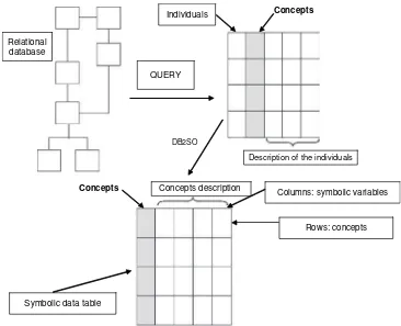
This book is based on the eight following steps described in Figure 1.5 (which will be detailed in Chapter 24). First, a relational database is assumed to be given, composed of several more or less linked data tables (also called relations).
Second, a set of categories based on the categorical variables values of the database are chosen by an expert. For example, from the Cartesian product age × gender, with three levels of age (young if less then 35, age between 35 and 70, old if more than 70), six categories are obtained.
Third, from a query to the given relational database, a data table is obtained whose first column represents the individuals (no more than one row for each individual), and whose second column represents a categorical variable and associates with each individual its unique category. Each category is associated with its ‘extent’ in the database. This extent
QUERY
DB2SO
Concepts
Concepts
Concepts description Columns: symbolic variables
Rows: concepts Relational
database
Individuals
Description of the individuals
Symbolic data table
is defined by the set of individuals which satisfy the category. For example, a male aged 20 is an individual who satisfies the category (male, young).
Fourth, the class of individuals which defines the extent of a category is considered to be the extent of the concept which reifies this category.
Fifth, a generalization process is defined, in order to associate a description with any subset of individuals.
Sixth, the generalization process is applied to the subset of individuals belonging to the extent of each concept. The description produced by this generalization process is considered to be a description of each concept. This step is provided in SODAS2 by the DB2SO module (see Chapter 2). As already noted, the generalization process must take into account the internal variation of the set of individuals that it describes and leads to symbolic variables and symbolic data.
Seventh, a symbolic data table, where the units are the concepts and the variables are the symbolic variables which describe them, is defined. Conceptual variables can be added at the concept level, as can any required background knowledge (rules and taxonomies).
Eighth, symbolic data analysis tools such as those explained in this book are applied on this symbolic data table by taking the background knowledge into account.
1.5.3 From data mining to knowledge mining by symbolic data
analysis: main principles
In order to apply the tools of standard data mining (clustering, decision trees, factor analysis, rule extraction, ) to concepts, these tools must be extended to symbolic data. The main
principles of a symbolic data analysis can be summarized by the following steps:
1. A symbolic data analysis needs two levels of units. The first level is that of individuals, the second that of concepts.
2. A concept is described by using the symbolic description of a class of individuals defined by the extent of a category.
3. The description of a concept must take account of the variation of the individuals of its extent.
4. A concept can be modelled by a symbolic object which can be improved in a learning process (based on the schema of Figure 1.6 explained in the next section), taking into account the arrival of new individuals.
5. Symbolic data analysis extends standard exploratory data analysis and data mining to the case where the units are concepts described by symbolic data.
6. The output of some methods of symbolic data analysis (clustering, symbolic Galois lattice, decision trees, Kohonen maps, etc.) provides new symbolic objects associated with new categories (i.e., categories of concepts).
MODELLING CONCEPTS BY SYMBOLIC OBJECTS 23
1.5.4 Is there a general theory of symbolic data analysis?
As it is not possible to say that there is a general theory of standard statistics, it follows that we also cannot say that there is a general theory of symbolic data analysis. The aim, in both cases, is to solve problems arising from the data by using the most appropriate mathematical theory. However, we can say that in symbolic data analysis, like the units, the theory increases in generality. For example, if we consider the marks achieved by Tom, Paul and Paula at each physics and mathematics examination taken during a given year, we are able to define a standard numerical data table withnrows (the number of exams) and two columns defined by two numerical random variablesXP andXMwhich associate with each exam taken by Tom (or Paul or Paula), the marks achieved in physics and mathematics. Thus XP(exami, Tom) =15 means that Tom scored 15 in mathematics at the ith examination.
Now, if we consider that Tom, Paul and Paula are three concepts, then we obtain a new data table with three rows associated with each pupil and two columns associated with two new variables YP and YM for which the values are the preceding random variables where the name of the pupil is fixed. For example,YP(Tom)=XP(·, Tom). If we replace, in each cell of this data table, the random variable that it contains with the confidence interval of its associated distribution, we obtain an example of symbolic data table where each variable is interval-valued.
1.6 Modelling concepts by symbolic objects
1.6.1 Modelling description by the joint or by the margins
A natural way to model the intent of a concept (in order to be able to obtain its extent) is to give a description of a class of individuals of its extent (for example, the penguins of an island in order to model the concept of ‘penguin’). From a statistical point of view there are two extreme ways to describe such a class.
The first is to describe it by the joint distribution of all the variables (if the variables are a mixture of numerical and categorical, it is always possible to transform them so that they all become categorical). In this case, the problem is that the space tends to become empty as the number of variables becomes large, which is one of the characteristics of data mining.
The second is to describe this class of individuals by the margins associated with all available descriptive variables. In this case, some joint information is lost but easy interpretable results are obtained, as the variables are transparent instead of being hidden in a joint distribution.
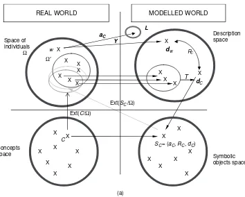
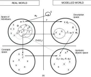
1.6.2 The four basic spaces for modelling concepts by symbolic objects
In Figure 1.6 the ‘set of individuals’ and the ‘set of concepts’ constitute the ‘real world’ set; we might say that the ‘world of objects in the real world: the individuals and concepts’ are considered as lower and higher-level objects. The ‘modelled world’ is composed of the ‘set of descriptions’ which models individuals (or classes of individuals) and the ‘set of symbolic objects’ which models concepts. In Figure 1.6(a) the starting point is a conceptC whose extent, denoted Ext(C/′), is known in a sample′of individuals. In Figure 1.6(b) the starting point is a given class of individuals associated with a conceptC.If the conceptCis the swallow species, and 30 individual swallows have been captured among a sample′of the swallows of an island, Ext(C/′) is known to be composed of these 30 swallows (Figure 1.6(a)). Each individualwin the extent ofC in′is described in the ‘description space’ by using the mappingysuch thatyw=dwdescribes the individualw.
Given a class of 30 similar birds obtained, for example, from a clustering process, a concept called ‘swallow’ is associated with this class (Figure 1.6(b)). Each individualwin this class is described in the ‘description space’ by using the mappingysuch thatyw=dw
describes the individualw.
The conceptCis modelled in the set of symbolic objects by the following steps described in Figure 1.6.
MODELLING CONCEPTS BY SYMBOLIC OBJECTS 25
Figure 1.6 (b) Modellization by a concept known by a class of individuals.
First, the set of descriptions of the individuals of Ext(C/′) in Figure 1.6(a), or of the class of individuals associated with the concept C in Figure 1.6(b), is generalized with an operatorT in order to produce the descriptiondC(which may be a set of Cartesian products
of intervals and/or distributions or just a unique joint distribution, etc.).
Second, the matching relation R can be chosen in relation to the choice of T. For instance, ifT= ∪, thenRC= ‘⊆’; ifT= ∩, thenR=‘⊇’ (see Section 1.7). The membership
function is then defined by the mappingaC:→LwhereLis [0, 1] or {true, false} such that
aCw=yw RCdCwhich measures the fit or match between the descriptionyw=dw
of the unit w and the descriptiondC of the extent of the conceptC in the database. The
symbolic object modelling the conceptC by the triples=aC R dCcan then be defined. In the next section, this definition is considered again and illustrated by several examples. Sometimes the following question arises: ‘why not reduce the modelling of the conceptC to just the membership functionaCas it suffices to knowaCin order to obtain the extent?’. The reason is that in this case we would not know which kind of descriptiondCis associated
with the concept nor which kind of matching relation R is used as several dC or R can