Methods of Multivariate Analysis
Second Edition
ALVIN C. RENCHER Brigham Young University
Copyright c2002 by John Wiley & Sons, Inc. All rights reserved. Published simultaneously in Canada.
No part of this publication may be reproduced, stored in a retrieval system or transmitted in any form or by any means, electronic, mechanical, photocopying, recording, scanning or otherwise, except as permitted under Sections 107 or 108 of the 1976 United States Copyright Act, without either the prior written permission of the Publisher, or authorization through payment of the appropriate per-copy fee to the Copyright Clearance Center, 222 Rosewood Drive, Danvers, MA 01923, (978) 750-8400, fax (978) 750-4744. Requests to the Publisher for permission should be addressed to the Permissions Department, John Wiley & Sons, Inc., 605 Third Avenue, New York, NY 10158-0012, (212) 850-6011, fax (212) 850-6008. E-Mail: [email protected].
For ordering and customer service, call 1-800-CALL-WILEY. Library of Congress Cataloging-in-Publication Data Rencher, Alvin C., 1934–
Methods of multivariate analysis / Alvin C. Rencher.—2nd ed. p. cm. — (Wiley series in probability and mathematical statistics) “A Wiley-Interscience publication.”
Includes bibliographical references and index. ISBN 0-471-41889-7 (cloth)
1. Multivariate analysis. I. Title. II. Series. QA278 .R45 2001
519.5′35—dc21 2001046735
1. Introduction 1
1.1 Why Multivariate Analysis?, 1 1.2 Prerequisites, 3
1.3 Objectives, 3
1.4 Basic Types of Data and Analysis, 3
2. Matrix Algebra 5
2.1 Introduction, 5
2.2 Notation and Basic Definitions, 5
2.2.1 Matrices, Vectors, and Scalars, 5 2.2.2 Equality of Vectors and Matrices, 7 2.2.3 Transpose and Symmetric Matrices, 7 2.2.4 Special Matrices, 8
2.3 Operations, 9
2.3.1 Summation and Product Notation, 9 2.3.2 Addition of Matrices and Vectors, 10 2.3.3 Multiplication of Matrices and Vectors, 11 2.4 Partitioned Matrices, 20
2.5 Rank, 22 2.6 Inverse, 23
2.7 Positive Definite Matrices, 25 2.8 Determinants, 26
2.9 Trace, 30
2.10 Orthogonal Vectors and Matrices, 31 2.11 Eigenvalues and Eigenvectors, 32
2.11.1 Definition, 32 2.11.2 I+AandI−A, 33 2.11.3 tr(A)and|A|, 34
2.11.4 Positive Definite and Semidefinite Matrices, 34 2.11.5 The ProductAB, 35
2.11.6 Symmetric Matrix, 35
2.11.7 Spectral Decomposition, 35 2.11.8 Square Root Matrix, 36
2.11.9 Square Matrices and Inverse Matrices, 36 2.11.10 Singular Value Decomposition, 36
3. Characterizing and Displaying Multivariate Data 43 3.1 Mean and Variance of a Univariate Random Variable, 43
3.2 Covariance and Correlation of Bivariate Random Variables, 45 3.2.1 Covariance, 45
3.2.2 Correlation, 49
3.3 Scatter Plots of Bivariate Samples, 50
3.4 Graphical Displays for Multivariate Samples, 52 3.5 Mean Vectors, 53
3.6 Covariance Matrices, 57 3.7 Correlation Matrices, 60
3.8 Mean Vectors and Covariance Matrices for Subsets of Variables, 62
3.8.1 Two Subsets, 62
3.8.2 Three or More Subsets, 64 3.9 Linear Combinations of Variables, 66
3.9.1 Sample Properties, 66 3.9.2 Population Properties, 72 3.10 Measures of Overall Variability, 73 3.11 Estimation of Missing Values, 74 3.12 Distance between Vectors, 76
4. The Multivariate Normal Distribution 82
4.1 Multivariate Normal Density Function, 82 4.1.1 Univariate Normal Density, 82 4.1.2 Multivariate Normal Density, 83 4.1.3 Generalized Population Variance, 83
4.1.4 Diversity of Applications of the Multivariate Normal, 85 4.2 Properties of Multivariate Normal Random Variables, 85
4.3 Estimation in the Multivariate Normal, 90 4.3.1 Maximum Likelihood Estimation, 90 4.3.2 Distribution ofyandS, 91
4.4 Assessing Multivariate Normality, 92
4.5 Outliers, 99
4.5.1 Outliers in Univariate Samples, 100 4.5.2 Outliers in Multivariate Samples, 101
5. Tests on One or Two Mean Vectors 112
5.1 Multivariate versus Univariate Tests, 112 5.2 Tests onwith⌺Known, 113
5.2.1 Review of Univariate Test forH0:µ=µ0 withσKnown, 113
5.2.2 Multivariate Test forH0:=0with⌺Known, 114 5.3 Tests onWhen⌺Is Unknown, 117
5.3.1 Review of Univariatet-Test forH0:µ=µ0withσ Unknown, 117
5.3.2 Hotelling’sT2-Test forH0:=0with⌺Unknown, 117 5.4 Comparing Two Mean Vectors, 121
5.4.1 Review of Univariate Two-Samplet-Test, 121 5.4.2 Multivariate Two-SampleT2-Test, 122 5.4.3 Likelihood Ratio Tests, 126
5.5 Tests on Individual Variables Conditional on Rejection ofH0by theT2-Test, 126
5.6 Computation ofT2, 130
5.6.1 ObtainingT2from a MANOVA Program, 130 5.6.2 ObtainingT2from Multiple Regression, 130 5.7 Paired Observations Test, 132
5.7.1 Univariate Case, 132 5.7.2 Multivariate Case, 134 5.8 Test for Additional Information, 136 5.9 Profile Analysis, 139
5.9.1 One-Sample Profile Analysis, 139 5.9.2 Two-Sample Profile Analysis, 141
6. Multivariate Analysis of Variance 156
6.1 One-Way Models, 156
6.1.1 Univariate One-Way Analysis of Variance (ANOVA), 156 6.1.2 Multivariate One-Way Analysis of Variance Model
(MANOVA), 158 6.1.3 Wilks’ Test Statistic, 161 6.1.4 Roy’s Test, 164
6.1.6 Unbalanced One-Way MANOVA, 168
6.1.7 Summary of the Four Tests and Relationship toT2, 168 6.1.8 Measures of Multivariate Association, 173
6.2 Comparison of the Four Manova Test Statistics, 176 6.3 Contrasts, 178
6.3.1 Univariate Contrasts, 178 6.3.2 Multivariate Contrasts, 180
6.4 Tests on Individual Variables Following Rejection ofH0by the Overall MANOVA Test, 183
6.5 Two-Way Classification, 186
6.5.1 Review of Univariate Two-Way ANOVA, 186 6.5.2 Multivariate Two-Way MANOVA, 188 6.6 Other Models, 195
6.6.1 Higher Order Fixed Effects, 195 6.6.2 Mixed Models, 196
6.7 Checking on the Assumptions, 198 6.8 Profile Analysis, 199
6.9 Repeated Measures Designs, 204
6.9.1 Multivariate vs. Univariate Approach, 204 6.9.2 One-Sample Repeated Measures Model, 208 6.9.3 k-Sample Repeated Measures Model, 211 6.9.4 Computation of Repeated Measures Tests, 212 6.9.5 Repeated Measures with Two Within-Subjects
Factors and One Between-Subjects Factor, 213 6.9.6 Repeated Measures with Two Within-Subjects
Factors and Two Between-Subjects Factors, 219 6.9.7 Additional Topics, 221
6.10 Growth Curves, 221
6.10.1 Growth Curve for One Sample, 221 6.10.2 Growth Curves for Several Samples, 229 6.10.3 Additional Topics, 230
6.11 Tests on a Subvector, 231
6.11.1 Test for Additional Information, 231 6.11.2 Stepwise Selection of Variables, 233
7. Tests on Covariance Matrices 248
7.1 Introduction, 248
7.2.2 Testing Sphericity, 250
7.2.3 TestingH0:⌺=σ2[(1−ρ)I+ρJ], 252 7.3 Tests Comparing Covariance Matrices, 254
7.3.1 Univariate Tests of Equality of Variances, 254
7.3.2 Multivariate Tests of Equality of Covariance Matrices, 255 7.4 Tests of Independence, 259
7.4.1 Independence of Two Subvectors, 259 7.4.2 Independence of Several Subvectors, 261 7.4.3 Test for Independence of All Variables, 265
8. Discriminant Analysis: Description of Group Separation 270 8.1 Introduction, 270
8.2 The Discriminant Function for Two Groups, 271
8.3 Relationship between Two-Group Discriminant Analysis and Multiple Regression, 275
8.4 Discriminant Analysis for Several Groups, 277 8.4.1 Discriminant Functions, 277
8.4.2 A Measure of Association for Discriminant Functions, 282 8.5 Standardized Discriminant Functions, 282
8.6 Tests of Significance, 284
8.6.1 Tests for the Two-Group Case, 284 8.6.2 Tests for the Several-Group Case, 285 8.7 Interpretation of Discriminant Functions, 288
8.7.1 Standardized Coefficients, 289 8.7.2 PartialF-Values, 290
8.7.3 Correlations between Variables and Discriminant Functions, 291
8.7.4 Rotation, 291 8.8 Scatter Plots, 291
8.9 Stepwise Selection of Variables, 293
9. Classification Analysis: Allocation of Observations to Groups 299 9.1 Introduction, 299
9.2 Classification into Two Groups, 300 9.3 Classification into Several Groups, 304
9.3.1 Equal Population Covariance Matrices: Linear Classification Functions, 304
9.4 Estimating Misclassification Rates, 307 9.5 Improved Estimates of Error Rates, 309 9.5.1 Partitioning the Sample, 310 9.5.2 Holdout Method, 310 9.6 Subset Selection, 311
9.7 Nonparametric Procedures, 314 9.7.1 Multinomial Data, 314
9.7.2 Classification Based on Density Estimators, 315 9.7.3 Nearest Neighbor Classification Rule, 318
10. Multivariate Regression 322
10.1 Introduction, 322
10.2 Multiple Regression: Fixedx’s, 323 10.2.1 Model for Fixedx’s, 323
10.2.2 Least Squares Estimation in the Fixed-xModel, 324 10.2.3 An Estimator forσ2, 326
10.2.4 The Model Corrected for Means, 327 10.2.5 Hypothesis Tests, 329
10.2.6 R2in Fixed-xRegression, 332 10.2.7 Subset Selection, 333
10.3 Multiple Regression: Randomx’s, 337
10.4 Multivariate Multiple Regression: Estimation, 337 10.4.1 The Multivariate Linear Model, 337
10.4.2 Least Squares Estimation in the Multivariate Model, 339 10.4.3 Properties of Least Squares EstimatorsB, 341ˆ
10.4.4 An Estimator for⌺, 342 10.4.5 Model Corrected for Means, 342
10.5 Multivariate Multiple Regression: Hypothesis Tests, 343 10.5.1 Test of Overall Regression, 343
10.5.2 Test on a Subset of thex’s, 347
10.6 Measures of Association between they’s and thex’s, 349 10.7 Subset Selection, 351
10.7.1 Stepwise Procedures, 351 10.7.2 All Possible Subsets, 355 10.8 Multivariate Regression: Randomx’s, 358
11. Canonical Correlation 361
11.1 Introduction, 361
11.3 Properties of Canonical Correlations, 366 11.4 Tests of Significance, 367
11.4.1 Tests of No Relationship between they’s and thex’s, 367 11.4.2 Test of Significance of Succeeding Canonical
Correlations after the First, 369 11.5 Interpretation, 371
11.5.1 Standardized Coefficients, 371
11.5.2 Correlations between Variables and Canonical Variates, 373 11.5.3 Rotation, 373
11.5.4 Redundancy Analysis, 373
11.6 Relationships of Canonical Correlation Analysis to Other Multivariate Techniques, 374
11.6.1 Regression, 374
11.6.2 MANOVA and Discriminant Analysis, 376
12. Principal Component Analysis 380
12.1 Introduction, 380
12.2 Geometric and Algebraic Bases of Principal Components, 381 12.2.1 Geometric Approach, 381
12.2.2 Algebraic Approach, 385
12.3 Principal Components and Perpendicular Regression, 387 12.4 Plotting of Principal Components, 389
12.5 Principal Components from the Correlation Matrix, 393 12.6 Deciding How Many Components to Retain, 397 12.7 Information in the Last Few Principal Components, 401 12.8 Interpretation of Principal Components, 401
12.8.1 Special Patterns inSorR, 402 12.8.2 Rotation, 403
12.8.3 Correlations between Variables and Principal Components, 403
12.9 Selection of Variables, 404
13. Factor Analysis 408
13.1 Introduction, 408
13.2 Orthogonal Factor Model, 409
13.2.1 Model Definition and Assumptions, 409 13.2.2 Nonuniqueness of Factor Loadings, 414 13.3 Estimation of Loadings and Communalities, 415
13.3.3 Iterated Principal Factor Method, 424 13.3.4 Maximum Likelihood Method, 425 13.4 Choosing the Number of Factors,m, 426 13.5 Rotation, 430
13.5.1 Introduction, 430 13.5.2 Orthogonal Rotation, 431 13.5.3 Oblique Rotation, 435 13.5.4 Interpretation, 438 13.6 Factor Scores, 438
13.7 Validity of the Factor Analysis Model, 443
13.8 The Relationship of Factor Analysis to Principal Component Analysis, 447
14. Cluster Analysis 451
14.1 Introduction, 451
14.2 Measures of Similarity or Dissimilarity, 452 14.3 Hierarchical Clustering, 455
14.3.1 Introduction, 455
14.3.2 Single Linkage (Nearest Neighbor), 456 14.3.3 Complete Linkage (Farthest Neighbor), 459 14.3.4 Average Linkage, 463
14.3.5 Centroid, 463 14.3.6 Median, 466 14.3.7 Ward’s Method, 466 14.3.8 Flexible Beta Method, 468
14.3.9 Properties of Hierarchical Methods, 471 14.3.10 Divisive Methods, 479
14.4 Nonhierarchical Methods, 481 14.4.1 Partitioning, 481 14.4.2 Other Methods, 490 14.5 Choosing the Number of Clusters, 494 14.6 Cluster Validity, 496
14.7 Clustering Variables, 497
15. Graphical Procedures 504
15.1 Multidimensional Scaling, 504 15.1.1 Introduction, 504
15.2 Correspondence Analysis, 514 15.2.1 Introduction, 514
15.2.2 Row and Column Profiles, 515 15.2.3 Testing Independence, 519
15.2.4 Coordinates for Plotting Row and Column Profiles, 521 15.2.5 Multiple Correspondence Analysis, 526
15.3 Biplots, 531
15.3.1 Introduction, 531
15.3.2 Principal Component Plots, 531
15.3.3 Singular Value Decomposition Plots, 532 15.3.4 Coordinates, 533
15.3.5 Other Methods, 535
A. Tables 549
B. Answers and Hints to Problems 591
C. Data Sets and SAS Files 679
References 681
I have long been fascinated by the interplay of variables in multivariate data and by the challenge of unraveling the effect of each variable. My continuing objective in the second edition has been to present the power and utility of multivariate analysis in a highly readable format.
Practitioners and researchers in all applied disciplines often measure several vari-ables on each subject or experimental unit. In some cases, it may be productive to isolate each variable in a system and study it separately. Typically, however, the vari-ables are not only correlated with each other, but each variable is influenced by the other variables as it affects a test statistic or descriptive statistic. Thus, in many instances, the variables are intertwined in such a way that when analyzed individ-ually they yield little information about the system. Using multivariate analysis, the variables can be examined simultaneously in order to access the key features of the process that produced them. The multivariate approach enables us to (1) explore the joint performance of the variables and (2) determine the effect of each variable in the presence of the others.
Multivariate analysis provides both descriptive and inferential procedures—we can search for patterns in the data or test hypotheses about patterns of a priori inter-est. With multivariate descriptive techniques, we can peer beneath the tangled web of variables on the surface and extract the essence of the system. Multivariate inferential procedures include hypothesis tests that (1) process any number of variables without inflating the Type I error rate and (2) allow for whatever intercorrelations the vari-ables possess. A wide variety of multivariate descriptive and inferential procedures is readily accessible in statistical software packages.
My selection of topics for this volume reflects many years of consulting with researchers in many fields of inquiry. A brief overview of multivariate analysis is given in Chapter 1. Chapter 2 reviews the fundamentals of matrix algebra. Chapters 3 and 4 give an introduction to sampling from multivariate populations. Chapters 5, 6, 7, 10, and 11 extend univariate procedures with one dependent variable (including t-tests, analysis of variance, tests on variances, multiple regression, and multiple cor-relation) to analogous multivariate techniques involving several dependent variables. A review of each univariate procedure is presented before covering the multivariate counterpart. These reviews may provide key insights the student missed in previous courses.
find functions of the variables that reveal the basic dimensionality and characteristic patterns of the data, and we discuss procedures for finding the underlying latent variables of a system. In Chapters 14 and 15 (new in the second edition), we give methods for searching for groups in the data, and we provide plotting techniques that show relationships in a reduced dimensionality for various kinds of data.
In Appendix A, tables are provided for many multivariate distributions and tests. These enable the reader to conduct an exact test in many cases for which software packages provide only approximate tests. Appendix B gives answers and hints for most of the problems in the book.
Appendix C describes an ftp site that contains (1) all data sets and (2) SAS com-mand files for all examples in the text. These comcom-mand files can be adapted for use in working problems or in analyzing data sets encountered in applications.
To illustrate multivariate applications, I have provided many examples and exer-cises based on 59 real data sets from a wide variety of disciplines. A practitioner or consultant in multivariate analysis gains insights and acumen from long experi-ence in working with data. It is not expected that a student can achieve this kind of seasoning in a one-semester class. However, the examples provide a good start, and further development is gained by working problems with the data sets. For example, in Chapters 12 and 13, the exercises cover several typical patterns in the covariance or correlation matrix. The student’s intuition is expanded by associating these covari-ance patterns with the resulting configuration of the principal components or factors. Although this is a methods book, I have included a few derivations. For some readers, an occasional proof provides insights obtainable in no other way. I hope that instructors who do not wish to use proofs will not be deterred by their presence. The proofs can be disregarded easily when reading the book.
My objective has been to make the book accessible to readers who have taken as few as two statistical methods courses. The students in my classes in multivariate analysis include majors in statistics and majors from other departments. With the applied researcher in mind, I have provided careful intuitive explanations of the con-cepts and have included many insights typically available only in journal articles or in the minds of practitioners.
My overriding goal in preparation of this book has been clarity of exposition. I hope that students and instructors alike will find this multivariate text more com-fortable than most. In the final stages of development of both the first and second editions, I asked my students for written reports on their initial reaction as they read each day’s assignment. They made many comments that led to improvements in the manuscript. I will be very grateful if readers will take the time to notify me of errors or of other suggestions they might have for improvements.
I have tried to use standard mathematical and statistical notation as far as pos-sible and to maintain consistency of notation throughout the book. I have refrained from the use of abbreviations and mnemonic devices. These save space when one is reading a book page by page, but they are annoying to those using a book as a reference.
num-bered sequentially throughout a chapter in the form “Table 3.8” or “Figure 3.1.” Examples are not numbered sequentially; each example is identified by the same number as the section in which it appears and is placed at the end of the section.
When citing references in the text, I have used the standard format involving the year of publication. For a journal article, the year alone suffices, for example, Fisher (1936). But for books, I have usually included a page number, as in Seber (1984, p. 216).
This is the first volume of a two-volume set on multivariate analysis. The second volume is entitledMultivariate Statistical Inference and Applications(Wiley, 1998). The two volumes are not necessarily sequential; they can be read independently. I adopted the two-volume format in order to (1) provide broader coverage than would be possible in a single volume and (2) offer the reader a choice of approach.
The second volume includes proofs of many techniques covered in the first 13 chapters of the present volume and also introduces additional topics. The present volume includes many examples and problems using actual data sets, and there are fewer algebraic problems. The second volume emphasizes derivations of the results and contains fewer examples and problems with real data. The present volume has fewer references to the literature than the other volume, which includes a careful review of the latest developments and a more comprehensive bibliography. In this second edition, I have occasionally referred the reader to Rencher (1998) to note that added coverage of a certain subject is available in the second volume.
I am indebted to many individuals in the preparation of the first edition. My ini-tial exposure to multivariate analysis came in courses taught by Rolf Bargmann at the University of Georgia and D. R. Jensen at Virginia Tech. Additional impetus to probe the subtleties of this field came from research conducted with Bruce Brown at BYU. I wish to thank Bruce Brown, Deane Branstetter, Del Scott, Robert Smidt, and Ingram Olkin for reading various versions of the manuscript and making valu-able suggestions. I am grateful to the following students at BYU who helped with computations and typing: Mitchell Tolland, Tawnia Newton, Marianne Matis Mohr, Gregg Littlefield, Suzanne Kimball, Wendy Nielsen, Tiffany Nordgren, David Whit-ing, Karla Wasden, and Rachel Jones.
SECOND EDITION
For the second edition, I have added Chapters 14 and 15, covering cluster analysis, multidimensional scaling, correspondence analysis, and biplots. I also made numer-ous corrections and revisions (almost every page) in the first 13 chapters, in an effort to improve composition, readability, and clarity. Many of the first 13 chapters now have additional problems.
I have listed the data sets and SAS files on the Wiley ftp site rather than on a diskette, as in the first edition. I have made improvements in labeling of these files.
I thank Lonette Stoddard and Candace B. McNaughton for typing and J. D. Williams for computer support. As with my other books, I dedicate this volume to my wife, LaRue, who has supplied much needed support and encouragement.
I thank the authors, editors, and owners of copyrights for permission to reproduce the following materials:
• Figure 3.8 and Table 3.2, Kleiner and Hartigan (1981), Reprinted by permission ofJournal of the American Statistical Association
• Table 3.3, Kramer and Jensen (1969a), Reprinted by permission ofJournal of Quality Technology
• Table 3.4, Reaven and Miller (1979), Reprinted by permission ofDiabetologia • Table 3.5, Timm (1975), Reprinted by permission of Elsevier North-Holland
Publishing Company
• Table 3.6, Elston and Grizzle (1962), Reprinted by permission ofBiometrics • Table 3.7, Frets (1921), Reprinted by permission ofGenetica
• Table 3.8, O’Sullivan and Mahan (1966), Reprinted by permission ofAmerican Journal of Clinical Nutrition
• Table 4.3, Royston (1983), Reprinted by permission ofApplied Statistics • Table 5.1, Beall (1945), Reprinted by permission ofPsychometrika
• Table 5.2, Hummel and Sligo (1971), Reprinted by permission ofPsychological Bulletin
• Table 5.3, Kramer and Jensen (1969b), Reprinted by permission ofJournal of Quality Technology
• Table 5.5, Lubischew (1962), Reprinted by permission ofBiometrics • Table 5.6, Travers (1939), Reprinted by permission ofPsychometrika
• Table 5.7, Andrews and Herzberg (1985), Reprinted by permission of Springer-Verlag
• Table 5.8, Tintner (1946), Reprinted by permission ofJournal of the American Statistical Association
• Table 5.9, Kramer (1972), Reprinted by permission of the author
• Table 5.10, Cameron and Pauling (1978), Reprinted by permission of National Academy of Science
• Table 6.2, Andrews and Herzberg (1985), Reprinted by permission of Springer-Verlag
• Table 6.3, Rencher and Scott (1990), Reprinted by permission of Communica-tions in Statistics: Simulation and Computation
• Table 6.6, Posten (1962), Reprinted by permission of the author
• Table 6.8, Crowder and Hand (1990, pp. 21–29), Reprinted by permission of Routledge Chapman and Hall
• Table 6.12, Cochran and Cox (1957), Timm (1980), Reprinted by permission of John Wiley and Sons and Elsevier North-Holland Publishing Company
• Table 6.14, Timm (1980), Reprinted by permission of Elsevier North-Holland Publishing Company
• Table 6.16, Potthoff and Roy (1964), Reprinted by permission of Biometrika Trustees
• Table 6.17, Baten, Tack, and Baeder (1958), Reprinted by permission ofQuality Progress
• Table 6.18, Keuls et al. (1984), Reprinted by permission ofScientia Horticul-turae
• Table 6.19, Burdick (1979), Reprinted by permission of the author • Table 6.20, Box (1950), Reprinted by permission ofBiometrics
• Table 6.21, Rao (1948), Reprinted by permission of Biometrika Trustees • Table 6.22, Cameron and Pauling (1978), Reprinted by permission of National
Academy of Science
• Table 6.23, Williams and Izenman (1989), Reprinted by permission of Colorado State University
• Table 6.24, Beauchamp and Hoel (1974), Reprinted by permission ofJournal of Statistical Computation and Simulation
• Table 6.25, Box (1950), Reprinted by permission ofBiometrics
• Table 6.26, Grizzle and Allen (1969), Reprinted by permission ofBiometrics • Table 6.27, Crepeau et al. (1985), Reprinted by permission ofBiometrics • Table 6.28, Zerbe (1979a), Reprinted by permission ofJournal of the American
Statistical Association
• Table 6.29, Timm (1980), Reprinted by permission of Elsevier North-Holland Publishing Company
• Table 7.2, Reprinted by permission of R. J. Freund
• Table 8.1, Kramer and Jensen (1969a), Reprinted by permission ofJournal of Quality Technology
• Table 8.3, Reprinted by permission of G. R. Bryce and R. M. Barker
• Table 10.1, Box and Youle (1955), Reprinted by permission ofBiometrics • Tables 12.2, 12.3, and 12.4, Jeffers (1967), Reprinted by permission ofApplied
Statistics
• Table 13.1, Brown et al. (1984), Reprinted by permission of the Journal of Pascal, Ada, and Modula
• Correlation matrix in Example 13.6, Brown, Strong, and Rencher (1973), Reprinted by permission ofThe Journal of the Acoustical Society of America • Table 14.1, Hartigan (1975), Reprinted by permission of John Wiley and Sons
• Table 14.3, Dawkins (1989), Reprinted by permission ofThe American Statis-tician
• Table 14.7, Hand et al. (1994), Reprinted by permission of D. J. Hand
• Table 14.12, Sokol and Rohlf (1981), Reprinted by permission of W. H. Free-man and Co.
• Table 14.13, Hand et al. (1994), Reprinted by permission of D. J. Hand
• Table 15.1, Kruskal and Wish (1978), Reprinted by permission of Sage Publi-cations
• Tables 15.2 and 15.5, Hand et al. (1994), Reprinted by permission of D. J. Hand
• Table 15.13, Edwards and Kreiner (1983), Reprinted by permission ofBiometrika • Table 15.15, Hand et al. (1994), Reprinted by permission of D. J. Hand
• Table 15.16, Everitt (1987), Reprinted by permission of the author
• Table 15.17, Andrews and Herzberg (1985), Reprinted by permission of Springer Verlag
• Table 15.18, Clausen (1988), Reprinted by permission of Sage Publications
• Table 15.19, Andrews and Herzberg (1985), Reprinted by permission of Springer Verlag
• Table A.1, Mulholland (1977), Reprinted by permission of Biometrika Trustees
• Table A.2, D’Agostino and Pearson (1973), Reprinted by permission of Biometrika Trustees
• Table A.4, D’Agostino (1972), Reprinted by permission of Biometrika Trustees
• Table A.5, Mardia (1970, 1974), Reprinted by permission of Biometrika Trustees
• Table A.6, Barnett and Lewis (1978), Reprinted by permission of John Wiley and Sons
• Table A.7, Kramer and Jensen (1969a), Reprinted by permission ofJournal of Quality Technology
• Table A.8, Bailey (1977), Reprinted by permission of Journal of the American Statistical Association
• Table A.9, Wall (1967), Reprinted by permission of the author, Albuquerque, NM
• Table A.10, Pearson and Hartley (1972) and Pillai (1964, 1965), Reprinted by permission of Biometrika Trustees
• Table A.11, Schuurmann et al. (1975), Reprinted by permission ofJournal of Statistical Computation and Simulation
• Table A.12, Davis (1970a,b, 1980), Reprinted by permission of Biometrika Trustees
• Table A.13, Kleinbaum, Kupper, and Muller (1988), Reprinted by permission of PWS-KENT Publishing Company
• Table A.14, Lee et al. (1977), Reprinted by permission of Elsevier North-Holland Publishing Company
Introduction
1.1 WHY MULTIVARIATE ANALYSIS?
Multivariate analysis consists of a collection of methods that can be used when sev-eral measurements are made on each individual or object in one or more samples. We will refer to the measurements asvariablesand to the individuals or objects asunits (research units, sampling units, or experimental units) orobservations. In practice, multivariate data sets are common, although they are not always analyzed as such. But the exclusive use of univariate procedures with such data is no longer excusable, given the availability of multivariate techniques and inexpensive computing power to carry them out.
Historically, the bulk of applications of multivariate techniques have been in the behavioral and biological sciences. However, interest in multivariate methods has now spread to numerous other fields of investigation. For example, I have collab-orated on multivariate problems with researchers in education, chemistry, physics, geology, engineering, law, business, literature, religion, public broadcasting, nurs-ing, minnurs-ing, linguistics, biology, psychology, and many other fields. Table 1.1 shows some examples of multivariate observations.
The reader will notice that in some cases all the variables are measured in the same scale (see 1 and 2 in Table 1.1). In other cases, measurements are in different scales (see 3 in Table 1.1). In a few techniques, such as profile analysis (Sections 5.9 and 6.8), the variables must be commensurate, that is, similar in scale of measurement; however, most multivariate methods do not require this.
Ordinarily the variables are measured simultaneously on each sampling unit. Typ-ically, these variables are correlated. If this were not so, there would be little use for many of the techniques of multivariate analysis. We need to untangle the overlapping information provided by correlated variables and peer beneath the surface to see the underlying structure. Thus the goal of many multivariate approaches is simplifica-tion. We seek to express what is going on in terms of a reduced set of dimensions. Such multivariate techniques are exploratory; they essentially generate hypotheses rather than test them.
On the other hand, if our goal is a formal hypothesis test, we need a technique that will (1) allow several variables to be tested and still preserve the significance level
Table 1.1. Examples of Multivariate Data
Units Variables
1. Students Several exam scores in a single course
2. Students Grades in mathematics, history, music, art, physics 3. People Height, weight, percentage of body fat, resting heart
rate
4. Skulls Length, width, cranial capacity
5. Companies Expenditures for advertising, labor, raw materials 6. Manufactured items Various measurements to check on compliance with
specifications
7. Applicants for bank loans Income, education level, length of residence, savings account, current debt load
8. Segments of literature Sentence length, frequency of usage of certain words and of style characteristics
9. Human hairs Composition of various elements
10. Birds Lengths of various bones
and (2) do this for any intercorrelation structure of the variables. Many such tests are available.
As the two preceding paragraphs imply, multivariate analysis is concerned gener-ally with two areas,descriptiveandinferentialstatistics. In the descriptive realm, we often obtain optimal linear combinations of variables. The optimality criterion varies from one technique to another, depending on the goal in each case. Although linear combinations may seem too simple to reveal the underlying structure, we use them for two obvious reasons: (1) they have mathematical tractability (linear approxima-tions are used throughout all science for the same reason) and (2) they often perform well in practice. These linear functions may also be useful as a follow-up to infer-ential procedures. When we have a statistically significant test result that compares several groups, for example, we can find the linear combination (or combinations) of variables that led to rejection of the hypothesis. Then the contribution of each variable to these linear combinations is of interest.
In the inferential area, many multivariate techniques are extensions of univariate procedures. In such cases, we review the univariate procedure before presenting the analogous multivariate approach.
Multivariate inference is especially useful in curbing the researcher’s natural ten-dency to read too much into the data. Total control is provided for experimentwise error rate; that is, no matter how many variables are tested simultaneously, the value ofα(the significance level) remains at the level set by the researcher.
or observations are involved, can be quickly and easily carried out. Perhaps it is not premature to say that multivariate analysis has come of age.
1.2 PREREQUISITES
The mathematical prerequisite for reading this book is matrix algebra. Calculus is not used [with a brief exception in equation (4.29)]. But the basic tools of matrix algebra are essential, and the presentation in Chapter 2 is intended to be sufficiently complete so that the reader with no previous experience can master matrix manipulation up to the level required in this book.
The statistical prerequisites are basic familiarity with the normal distribution,
t-tests, confidence intervals, multiple regression, and analysis of variance. These techniques are reviewed as each is extended to the analogous multivariate procedure. This is a multivariate methods text. Most of the results are given without proof. In a few cases proofs are provided, but the major emphasis is on heuristic explanations. Our goal is an intuitive grasp of multivariate analysis, in the same mode as other statistical methods courses. Some problems are algebraic in nature, but the majority involve data sets to be analyzed.
1.3 OBJECTIVES
I have formulated three objectives that I hope this book will achieve for the reader. These objectives are based on long experience teaching a course in multivariate methods, consulting on multivariate problems with researchers in many fields, and guiding statistics graduate students as they consulted with similar clients.
The first objective is to gain a thorough understanding of the details of various multivariate techniques, their purposes, their assumptions, their limitations, and so on. Many of these techniques are related; yet they differ in some essential ways. We emphasize these similarities and differences.
The second objective is to be able to select one or more appropriate techniques for a given multivariate data set. Recognizing the essential nature of a multivariate data set is the first step in a meaningful analysis. We introduce basic types of multivariate data in Section 1.4.
The third objective is to be able to interpret the results of a computer analysis of a multivariate data set. Reading the manual for a particular program package is not enough to make an intelligent appraisal of the output. Achievement of the first objective and practice on data sets in the text should help achieve the third objective.
1.4 BASIC TYPES OF DATA AND ANALYSIS
oversimpli-fication and might prefer elaborate tree diagrams of data structure. However, many data sets can fit into one of these categories, and the simplicity of this structure makes it easier to remember. The four basic data types are as follows:
1. A single sample with several variables measured on each sampling unit (sub-ject or ob(sub-ject);
2. A single sample with two sets of variables measured on each unit; 3. Two samples with several variables measured on each unit;
4. Three or more samples with several variables measured on each unit.
Each data type has extensions, and various combinations of the four are possible. A few examples of analyses for each case are as follows:
1. A single sample with several variables measured on each sampling unit: (a) Test the hypothesis that the means of the variables have specified values. (b) Test the hypothesis that the variables are uncorrelated and have a common
variance.
(c) Find a small set of linear combinations of the original variables that sum-marizes most of the variation in the data (principal components).
(d) Express the original variables as linear functions of a smaller set of under-lying variables that account for the original variables and their intercorre-lations (factor analysis).
2. A single sample with two sets of variables measured on each unit:
(a) Determine the number, the size, and the nature of relationships between the two sets of variables (canonical correlation). For example, you may wish to relate a set of interest variables to a set of achievement variables. How much overall correlation is there between these two sets?
(b) Find a model to predict one set of variables from the other set (multivariate multiple regression).
3. Two samples with several variables measured on each unit:
(a) Compare the means of the variables across the two samples (Hotelling’s
T2-test).
(b) Find a linear combination of the variables that best separates the two sam-ples (discriminant analysis).
(c) Find a function of the variables that accurately allocates the units into the two groups (classification analysis).
4. Three or more samples with several variables measured on each unit:
(a) Compare the means of the variables across the groups (multivariate anal-ysis of variance).
Matrix Algebra
2.1 INTRODUCTION
This chapter introduces the basic elements of matrix algebra used in the remainder of this book. It is essentially a review of the requisite matrix tools and is not intended to be a complete development. However, it is sufficiently self-contained so that those with no previous exposure to the subject should need no other reference. Anyone unfamiliar with matrix algebra should plan to work most of the problems entailing numerical illustrations. It would also be helpful to explore some of the problems involving general matrix manipulation.
With the exception of a few derivations that seemed instructive, most of the results are given without proof. Some additional proofs are requested in the problems. For the remaining proofs, see any general text on matrix theory or one of the specialized matrix texts oriented to statistics, such as Graybill (1969), Searle (1982), or Harville (1997).
2.2 NOTATION AND BASIC DEFINITIONS
2.2.1 Matrices, Vectors, and Scalars
Amatrixis a rectangular or square array of numbers or variables arranged in rows and columns. We use uppercase boldface letters to represent matrices. All entries in matrices will be real numbers or variables representing real numbers. The elements of a matrix are displayed in brackets. For example, the ACT score and GPA for three students can be conveniently listed in the following matrix:
A=
23 3.54 29 3.81 18 2.75
. (2.1)
The elements ofAcan also be variables, representing possible values of ACT and GPA for three students:
A=
a11 a12 a21 a22 a31 a32
. (2.2)
In this double-subscript notation for the elements of a matrix, the first subscript indi-cates the row; the second identifies the column. The matrixAin (2.2) can also be expressed as
A=(ai j), (2.3)
whereai j is a general element.
With three rows and two columns, the matrix A in (2.1) or (2.2) is said to be 3×2. In general, if a matrixAhasnrows and pcolumns, it is said to ben× p. Alternatively, we say thesizeofAisn×p.
Avectoris a matrix with a single column or row. The following could be the test scores of a student in a course in multivariate analysis:
x=
98 86 93 97
. (2.4)
Variable elements in a vector can be identified by a single subscript:
x=
x1 x2 x3 x4
. (2.5)
We use lowercase boldface letters for column vectors. Row vectors are expressed as x′=(x1,x2,x3,x4) or as x′=(x1 x2 x3 x4),
wherex′ indicates thetranspose of x. The transpose operation is defined in Sec-tion 2.2.3.
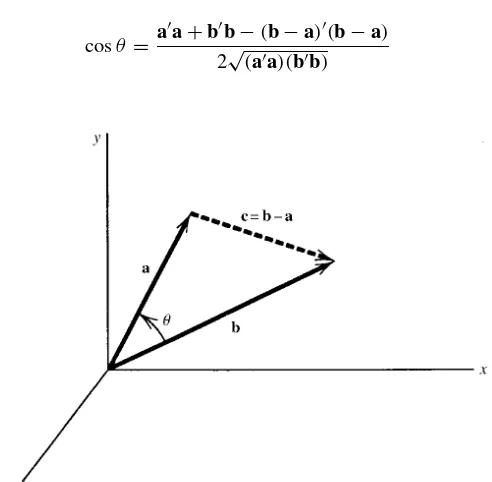
Geometrically, a vector with p elements identifies a point in a p-dimensional space. The elements in the vector are the coordinates of the point. In (2.35) in Sec-tion 2.3.3, we define the distance from the origin to the point. In SecSec-tion 3.12, we define the distance between two vectors. In some cases, we will be interested in a directed line segment or arrow from the origin to the point.
2.2.2 Equality of Vectors and Matrices
Two matrices are equal if they are the same size and the elements in corresponding positions are equal. Thus ifA=(ai j)andB=(bi j), thenA=Bifai j =bi jfor all two matrices are not the same size. Likewise,A= Dbecausea23 = d23. Thus two matrices of the same size are unequal if they differ in a single position.
2.2.3 Transpose and Symmetric Matrices
Thetransposeof a matrixA, denoted byA′, is obtained fromAby interchanging rows and columns. Thus the columns ofA′are the rows of A, and the rows of A′ are the columns ofA. The following examples illustrate the transpose of a matrix or vector:
The transpose operation does not change a scalar, since it has only one row and one column.
If the transpose operator is applied twice to any matrix, the result is the original matrix:
(A′)′=A. (2.6)
If the transpose of a matrix is the same as the original matrix, the matrix is said to besymmetric; that is,Ais symmetric ifA=A′. For example,
2.2.4 Special Matrices
Thediagonalof ap×psquare matrixAconsists of the elementsa11,a22, . . . ,app. For example, in the matrix
A=
the elements 5, 9, and 1 lie on the diagonal. If a matrix contains zeros in all off-diagonal positions, it is said to be adiagonal matrix. An example of a diagonal matrix is
This matrix can also be denoted as
D=diag(10,−3,0,7). (2.7) A diagonal matrix can be formed from any square matrix by replacing off-diagonal elements by 0’s. This is denoted by diag(A). Thus for the preceding matrix A, we have
A diagonal matrix with a 1 in each diagonal position is called anidentitymatrix and is denoted byI. For example, a 3×3 identity matrix is given by
I=
Anupper triangular matrixis a square matrix with zeros below the diagonal, such as
A vector of 1’s is denoted byj:
Finally, we denote a vector of zeros by0and a matrix of zeros byO. For example,
0=
2.3.1 Summation and Product Notation
For completeness, we review the standard mathematical notation for sums and prod-ucts. The sum of a sequence of numbersa1,a2, . . . ,anis indicated by
n i=1
ai =a1+a2+ · · · +an.
If thennumbers are all the same, thenni=1a=a+a+ · · · +a=na. The sum of all the numbers in an array with double subscripts, such as
a11 a12 a13
The product of a sequence of numbersa1,a2, . . . ,anis indicated by 2.3.2 Addition of Matrices and Vectors
If two matrices (or two vectors) are the same size, theirsum is found by adding corresponding elements; that is, ifAisn×pandBisn×p, thenC=A+Bis also
Similarly, thedifference between two matrices or two vectors of the same size is found by subtracting corresponding elements. ThusC=A−Bis found as(ci j)= (ai j −bi j). For example,
(3 9 −4)−(5 −4 2)=(−2 13 −6).
If two matrices are identical, their difference is a zero matrix; that is,A=Bimplies A−B=O. For example,
2.3.3 Multiplication of Matrices and Vectors
In order for the productABto be defined, the number of columns inAmust be the same as the number of rows inB, in which caseAandBare said to beconformable. Then the (i j)th element ofC=ABis
ci j = k
ai kbk j. (2.19)
Thusci j is the sum of products of theith row ofAand the jth column ofB. We therefore multiply each row ofAby each column ofB, and the size ofABconsists of the number of rows ofAand the number of columns ofB. Thus, ifAisn×mand
In some casesABis defined, butBAis not defined. In the preceding example,BA cannot be found becauseBis 3×2 andAis 4×3 and a row ofBcannot be multiplied by a column ofA. SometimesABandBAare both defined but are different in size. For example, ifAis 2×4 andBis 4×2, thenABis 2×2 andBAis 4×4. IfAand Bare square and the same size, thenABandBAare both defined. However,
AB=BA, (2.20)
except for a few special cases. For example, let
Then
Thus we must be careful to specify the order of multiplication. If we wish to multiply both sides of a matrix equation by a matrix, we must multiplyon the leftoron the rightand be consistent on both sides of the equation.
Multiplication is distributive over addition or subtraction:
A(B+C)=AB+AC, (2.21)
A(B−C)=AB−AC, (2.22)
(A+B)C=AC+BC, (2.23)
(A−B)C=AC−BC. (2.24)
Note that, in general, because of (2.20),
A(B+C)=BA+CA. (2.25)
Using the distributive law, we can expand products such as(A−B)(C−D)to obtain
(A−B)(C−D)=(A−B)C−(A−B)D [by (2.22)]
=AC−BC−AD+BD [by (2.24)]. (2.26) The transpose of a product is the product of the transposes in reverse order:
(AB)′=B′A′. (2.27)
c′A=(2 −5) The triple productc′Abwas obtained asc′(Ab). The same result would be obtained if we multiplied in the order(c′A)b: This is true in general for a triple product:
ABC=A(BC)=(AB)C. (2.28)
Thus multiplication of three matrices can be defined in terms of the product of two matrices, since (fortunately) it does not matter which two are multiplied first. Note that AandBmust be conformable for multiplication, and BandCmust be con-formable. For example, ifAisn×p,Bis p×q, andCisq×m, then both multi-plications are possible and the productABCisn×m.
We can sometimes factor a sum of triple products on both the right and left sides. For example,
ABC+ADC=A(B+D)C. (2.29)
As another illustration, letXben×pandAben×n. Then
Ifaandbare bothn×1, then
a′b=a1b1+a2b2+ · · · +anbn (2.31) is a sum of products and is a scalar. On the other hand,ab′is defined for any sizea andband is a matrix, either rectangular or square:
ab′= andaa′are sometimes referred to as thedot productandmatrix product, respectively. The square root of the sum of squares of the elements ofais thedistancefrom the origin to the pointaand is also referred to as thelengthofa:
j′A=
Sincea′bis a scalar, it is equal to its transpose:
a′b=(a′b)′=b′(a′)′=b′a. (2.39) This allows us to write(a′b)2in the form
(a′b)2
=(a′b)(a′b)=(a′b)(b′a)=a′(bb′)a. (2.40) From (2.18), (2.26), and (2.39) we obtain
(x−y)′(x−y)=x′x−2x′y+y′y. (2.41) Note that in analogous expressions with matrices, however, the two middle terms cannot be combined:
(A−B)′(A−B)=A′A−A′B−B′A+B′B,
(A−B)2=(A−B)(A−B)=A2−AB−BA+B2.
Ifaandx1,x2, . . . ,xnare allp×1 andAisp×p, we obtain the following factoring results as extensions of (2.21) and (2.29):
n
We can express matrix multiplication in terms of row vectors and column vectors. Ifa′
isa′
then the productABcan be written as
AB=
This can be expressed in terms of the rows ofA:
AB=
Note that the first column ofABin (2.46) is
and likewise the second column isAb2. ThusABcan be written in the form AB=A(b1,b2)=(Ab1,Ab2).
This result holds in general:
AB=A(b1,b2, . . . ,bp)=(Ab1,Ab2, . . . ,Abp). (2.48) To further illustrate matrix multiplication in terms of rows and columns, letA= a′
Similarly,
A′Ais p×pand is obtained as products of columns ofA[see (2.54)]. From (2.6) and (2.27), it is clear that bothAA′andA′Aare symmetric.
In the preceding illustration forABin terms of row and column vectors, the rows ofAwere denoted bya′i and the columns ofB, bybj. If both rows and columns of
With this notation for rows and columns ofA, we can express the elements of A′Aor ofAA′as products of the rows ofAor of the columns ofA. Thus if we write
then
d12a11 d1d2a12 d1d3a13 d2d1a21 d22a22 d2d3a23 d3d1a31 d3d2a32 d32a33
. (2.57)
In the special case where the diagonal matrix is the identity, we have
IA=AI=A. (2.58)
The product of a scalar and a matrix is obtained by multiplying each element of the matrix by the scalar:
cA=(cai j)=
Sincecai j =ai jc, the product of a scalar and a matrix is commutative:
cA=Ac. (2.62)
Multiplication of vectors or matrices by scalars permits the use of linear combi-nations, such as
IfAis a symmetric matrix andxandyare vectors, the product
y′Ay= i
aiiyi2+ i=j
ai jyiyj (2.63)
is called aquadratic form, whereas
x′Ay= i j
is called abilinear form. Either of these is, of course, a scalar and can be treated as such. Expressions such asx′Ay/√x′Ax are permissible (assumingAis positive definite; see Section 2.7).
2.4 PARTITIONED MATRICES
It is sometimes convenient to partition a matrix into submatrices. For example, a partitioning of a matrixAinto four submatrices could be indicated symbolically as follows:
For example, a 4×5 matrixAcan be partitioned as
A=
If two matricesAandBare conformable andAandBare partitioned so that the submatrices are appropriately conformable, then the productABcan be found by following the usual row-by-column pattern of multiplication on the submatrices as if they were single elements; for example,
AB=
Multiplication of a matrix and a vector can also be carried out in partitioned form.
where the partitioning of the columns ofA corresponds to the partitioning of the elements ofb. Note that the partitioning ofAinto two sets of columns is indicated by a comma,A=(A1,A2).
The partitioned multiplication in (2.66) can be extended to individual columns of Aand individual elements ofb:
Ab=(a1,a2, . . . ,ap) ThusAbis expressible as a linear combination of the columns ofA, the coefficients being elements ofb. For example, let
A=
Using a linear combination of columns ofAas in (2.67), we obtain
We note that ifAis partitioned as in (2.66),A=(A2,A2), the transpose is not equal to(A′
1,A′2), but rather
A′=(A1,A2)′=
A′ 1 A′
2
. (2.68)
2.5 RANK
Before defining the rank of a matrix, we first introduce the notion of linear inde-pendence and deinde-pendence. A set of vectorsa1, a2, . . . ,an is said to be linearly dependentif constantsc1,c2, . . . ,cn(not all zero) can be found such that
c1a1+c2a2+ · · · +cnan=0. (2.69) If no constantsc1,c2, . . . ,cncan be found satisfying (2.69), the set of vectors is said to belinearly independent.
If (2.69) holds, then at least one of the vectorsai can be expressed as a linear combination of the other vectors in the set. Thus linear dependence of a set of vec-tors implies redundancy in the set. Among linearly independent vecvec-tors there is no redundancy of this type.
Therankof any square or rectangular matrixAis defined as rank(A)=number of linearly independent rows ofA
=number of linearly independent columns ofA.
It can be shown that the number of linearly independent rows of a matrix is always equal to the number of linearly independent columns.
IfAisn×p, the maximum possible rank ofAis the smaller ofnandp, in which caseAis said to be offull rank(sometimes saidfull row rankorfull column rank). For example,
A=
1 −2 3
5 2 4
has rank 2 because the two rows are linearly independent (neither row is a multiple of the other). However, even thoughAis full rank, the columns are linearly dependent because rank 2 implies there are only two linearly independent columns. Thus, by (2.69), there exist constantsc1,c2, andc3such that
c1
1 5
+c2
−2
2
+c3
3 4
=
0 0
By (2.67), we can write (2.70) in the form Hence we have the interesting result that a product of a matrixAand a vectorcis equal to0, even thoughA=Oandc=0. This is a direct consequence of the linear dependence of the column vectors ofA.
Another consequence of the linear dependence of rows or columns of a matrix is the possibility of expressions such asAB=CB, whereA=C. For example, let
A=
All three matricesA,B, andCare full rank; but being rectangular, they have a rank deficiency in either rows or columns, which permits us to constructAB=CBwith A=C. Thus in a matrix equation, we cannot, in general, cancel matrices from both sides of the equation.
There are two exceptions to this rule. One exception involves a nonsingular matrix to be defined in Section 2.6. The other special case occurs when the expression holds for all possible values of the matrix common to both sides of the equation. For exam-ple,
IfAx=Bxfor all possible values ofx, thenA=B. (2.72) To see this, letx=(1,0, . . . ,0)′. Then the first column ofAequals the first column ofB. Now letx=(0,1,0, . . . ,0)′, and the second column ofAequals the second column ofB. Continuing in this fashion, we obtainA=B.
Suppose a rectangular matrixAisn×pof rankp, where p <n. We typically shorten this statement to “Aisn×pof rank p<n.”
2.6 INVERSE
If a matrixAis square and of full rank, thenAis said to benonsingular, andAhas a uniqueinverse, denoted byA−1, with the property that
For example, let
A=
3 4
2 6
.
Then
A−1=
.6 −.4
−.2 .3
,
AA−1=
3 4
2 6
.6 −.4
−.2 .3
=
1 0
0 1
.
IfAis square and of less than full rank, then an inverse does not exist, andAis said to besingular. Note that rectangular matrices do not have inverses as in (2.73), even if they are full rank.
IfAandBare the same size and nonsingular, then the inverse of their product is the product of their inverses in reverse order,
(AB)−1=B−1A−1. (2.74)
Note that (2.74) holds only for nonsingular matrices. Thus, for example, ifAisn×p of rank p < n, thenA′Ahas an inverse, but(A′A)−1is not equal to A−1(A′)−1 becauseAis rectangular and does not have an inverse.
If a matrix is nonsingular, it can be canceled from both sides of an equation, pro-vided it appears on the left (or right) on both sides. For example, ifBis nonsingular, then
AB=CB implies A=C, since we can multiply on the right byB−1to obtain
ABB−1=CBB−1, AI=CI,
A=C.
Otherwise, ifA,B, andCare rectangular or square and singular, it is easy to construct AB=CB, withA=C, as illustrated near the end of Section 2.5.
The inverse of the transpose of a nonsingular matrix is given by the transpose of the inverse:
(A′)−1=(A−1)′. (2.75)
If the symmetric nonsingular matrixAis partitioned in the form A=
A
11 a12 a′
12 a22
then the inverse is given by
A−1= 1 b
bA−1
11 +A −1
11a12a′12A −1 11 −A
−1 11a12 −a′
12A −1
11 1
, (2.76)
whereb=a22−a′12A−111a12. A nonsingular matrix of the formB+cc′, whereBis nonsingular, has as its inverse
(B+cc′)−1=B−1−B
−1cc′B−1
1+c′B−1c. (2.77)
2.7 POSITIVE DEFINITE MATRICES
The symmetric matrixAis said to bepositive definiteifx′Ax > 0 for all possible vectorsx(exceptx = 0). Similarly,Aispositive semidefiniteifx′Ax ≥ 0 for all x=0. [A quadratic formx′Axwas defined in (2.63).] The diagonal elementsaii of a positive definite matrix are positive. To see this, letx′=(0, . . . ,0,1,0, . . . ,0)with a 1 in theith position. Thenx′Ax=aii > 0. Similarly, for a positive semidefinite matrixA,aii ≥0 for alli.
One way to obtain a positive definite matrix is as follows:
IfA=B′B, whereBisn×pof rankp<n, thenB′Bis positive definite. (2.78) This is easily shown:
x′Ax=x′B′Bx=(Bx)′(Bx)=z′z,
wherez = Bx. Thusx′Ax = ni=1zi2, which is positive (Bx cannot be0unless x=0, becauseBis full rank). IfBis less than full rank, then by a similar argument, B′Bis positive semidefinite.
Note thatA=B′Bis analogous toa =b2in real numbers, where the square of any number (including negative numbers) is positive.
In another analogy to positive real numbers, a positive definite matrix can be factored into a “square root” in two ways. We give one method in (2.79) and the other in Section 2.11.8.
A positive definite matrixAcan be factored into
A=T′T, (2.79)
where T is a nonsingular upper triangular matrix. One way to obtain T is the Cholesky decomposition, which can be carried out in the following steps.
t11=√a11, t1j =
Then by the Cholesky method, we obtain
T=
Thedeterminantof ann×nmatrixAis defined as the sum of alln! possible products
ofnelements such that
1. each product contains one element from every row and every column, and 2. the factors in each product are written so that the column subscripts appear in
order of magnitude and each product is then preceded by a plus or minus sign according to whether the number of inversions in the row subscripts is even or odd.
Aninversionoccurs whenever a larger number precedes a smaller one. The symbol n!is defined as
The determinant ofAis a scalar denoted by|A|or by det(A). The preceding
def-inition is not useful in evaluating determinants, except in the case of 2×2 or 3×3 matrices. For larger matrices, other methods are available for manual computation, but determinants are typically evaluated by computer. For a 2×2 matrix, the deter-minant is found by
|A| =
a11 a12 a21 a22
=
a11a22−a21a12. (2.81)
For a 3×3 matrix, the determinant is given by
|A| =a11a22a33+a12a23a31+a13a32a21 −a31a22a13−a32a23a11−a33a12a21. (2.82)
This can be found by the following scheme. The three positive terms are obtained by
and the three negative terms, by
The determinant of a diagonal matrix is the product of the diagonal elements; that is, ifD=diag(d1,d2, . . . ,dn), then
|D| =
n i=1
di. (2.83)
As a special case of (2.83), suppose all diagonal elements are equal, say,
Then
|D| = |cI| =
n i=1
c=cn. (2.84)
The extension of (2.84) to any square matrixAis
|cA| =cn|A|. (2.85)
Since the determinant is a scalar, we can carry out operations such as |A|2, |A|1/2, 1
|A|,
provided that|A|>0 for|A|1/2and that|A| =0 for 1/|A|.
If the square matrixAis singular, its determinant is 0:
|A| =0 ifAis singular. (2.86)
IfAisnear singular, then there exists a linear combination of the columns that is
close to0, and|A|is also close to 0. IfAis nonsingular, its determinant is nonzero:
|A| =0 ifAis nonsingular. (2.87)
IfAis positive definite, its determinant is positive:
|A|>0 ifAis positive definite. (2.88)
If AandBare square and the same size, the determinant of the product is the
product of the determinants:
|AB| = |A||B|. (2.89)
For example, let
A=
1 2
−3 5
and B=
4 2 1 3
.
Then
AB=
6 8
−7 9
, |AB| =110,
|A| =11, |B| =10, |A||B| =110.
determinant:
|A′| = |A|, (2.90)
|A−1| = 1 |A| = |A|
−1. (2.91)
If a partitioned matrix has the form
A=
whereA11andA22are square but not necessarily the same size, then
|A| =
For a general partitioned matrix,
A=
whereA11 andA22are square and nonsingular (not necessarily the same size), the determinant is given by either of the following two expressions:
Note the analogy of (2.93) and (2.94) to the case of the determinant of a 2×2 matrix as given by (2.81):
IfBis nonsingular andcis a vector, then