Springer Algorithms And Data Structures The Basic Toolbox Aug 2008 ISBN 3540779779 pdf

(1)

(2)

(3)

(4)

Prof. Dr. Kurt Mehlhorn Prof. Dr. Peter Sanders Max-Planck-Institut für Informatik Universität Karlsruhe

Saarbrücken Germany

Germany sanders@ira.uka.de

mehlhorn@mpi-inf.mpg.de

ISBN 978-3-540-77977-3 e-ISBN 978-3-540-77978-0 DOI 10.1007/978-3-540-77978-0

Library of Congress Control Number: 2008926816

ACM Computing Classification (1998): F.2, E.1, E.2, G.2, B.2, D.1, I.2.8 c

2008 Springer-Verlag Berlin Heidelberg

This work is subject to copyright. All rights are reserved, whether the whole or part of the material is concerned, specifically the rights of translation, reprinting, reuse of illustrations, recitation, broadcasting, reproduction on microfilm or in any other way, and storage in data banks. Duplication of this publication or parts thereof is permitted only under the provisions of the German Copyright Law of September 9, 1965, in its current version, and permission for use must always be obtained from Springer. Violations are liable to prosecution under the German Copyright Law.

The use of general descriptive names, registered names, trademarks, etc. in this publication does not imply, even in the absence of a specific statement, that such names are exempt from the relevant protective laws and regulations and therefore free for general use.

Cover design:KünkelLopka GmbH, Heidelberg Printed on acid-free paper

(5)

(6)

Preface

Algorithms are at the heart of every nontrivial computer application. Therefore every computer scientist and every professional programmer should know about the basic algorithmic toolbox: structures that allow efficient organization and retrieval of data, frequently used algorithms, and generic techniques for modeling, understanding, and solving algorithmic problems.

This book is a concise introduction to this basic toolbox, intended for students and professionals familiar with programming and basic mathematical language. We have used the book in undergraduate courses on algorithmics. In our graduate-level courses, we make most of the book a prerequisite, and concentrate on the starred sections and the more advanced material. We believe that, even for undergraduates, a concise yet clear and simple presentation makes material more accessible, as long as it includes examples, pictures, informal explanations, exercises, and some linkage to the real world.

Most chapters have the same basic structure. We begin by discussing a problem as it occurs in a real-life situation. We illustrate the most important applications and then introduce simple solutionsas informally as possible and as formally as neces-saryto really understand the issues at hand. When we move to more advanced and optional issues, this approach gradually leads to a more mathematical treatment, in-cluding theorems and proofs. This way, the book should work for readers with a wide range of mathematical expertise. There are also advanced sections (marked with a *) where werecommendthat readers should skip them on first reading. Exercises pro-vide additional examples, alternative approaches and opportunities to think about the problems. It is highly recommended to take a look at the exercises even if there is no time to solve them during the first reading. In order to be able to concentrate on ideas rather than programming details, we use pictures, words, and high-level pseu-docode to explain our algorithms. A section “implementation notes” links these ab-stract ideas to clean, efficient implementations in real programming languages such as C++and Java. Each chapter ends with a section on further findings that provides a glimpse at the state of the art, generalizations, and advanced solutions.

(7)

way, including explicitly formulated invariants. We also discuss recent trends, such as algorithm engineering, memory hierarchies, algorithm libraries, and certifying algorithms.

We have chosen to organize most of the material by problem domain and not by solution technique. The final chapter on optimization techniques is an exception. We find that presentation by problem domain allows a more concise presentation. How-ever, it is also important that readers and students obtain a good grasp of the available techniques. Therefore, we have structured the final chapter by techniques, and an ex-tensive index provides cross-references between different applications of the same technique. Bold page numbers in the Index indicate the pages where concepts are defined.

Karlsruhe, Saarbrücken, Kurt Mehlhorn

(8)

Appetizer: Integer Arithmetics

An appetizer is supposed to stimulate the appetite at the beginning of a meal. This is exactly the purpose of this chapter. We want to stimulate your interest in algorithmic1 techniques by showing you a surprising result. The school method for multiplying in-tegers is not the best multiplication algorithm; there are much faster ways to multiply large integers, i.e., integers with thousands or even millions of digits, and we shall teach you one of them.

Arithmetic on long integers is needed in areas such as cryptography, geometric computing, and computer algebra and so an improved multiplication algorithm is not just an intellectual gem but also useful for applications. On the way, we shall learn basic analysis and basic algorithm engineering techniques in a simple setting. We shall also see the interplay of theory and experiment.

We assume that integers are represented as digit strings. In the baseBnumber system, whereBis an integer larger than one, there are digits 0, 1, toB−1 and a digit stringan−1an−2. . .a1a0represents the number∑0≤i<naiBi. The most important systems with a small value ofBare base 2, with digits 0 and 1, base 10, with digits 0 to 9, and base 16, with digits 0 to 15 (frequently written as 0 to 9, A, B, C, D, E, and F). Larger bases, such as 28, 216, 232, and 264, are also useful. For example,

“10101” in base 2 represents 1·24+0·23+1·22+0·21+1·20= 21, “924” in base 10 represents 9·102+2·101+4·100= 924.

(13)

multiplication of two digits with a two-digit result.2 For example, in base 10, we have

3 5 5 13

and 6·7=42.

We shall measure the efficiency of our algorithms by the number of primitive opera-tions executed.

We can artificially turn anyn-digit integer into anm-digit integer for anym≥nby adding additional leading zeros. Concretely, “425” and “000425” represent the same integer. We shall useaandbfor the two operands of an addition or multiplication and assume throughout this section thataandbaren-digit integers. The assumption that both operands have the same length simplifies the presentation without changing the key message of the chapter. We shall come back to this remark at the end of the chapter. We refer to the digits ofaasan−1toa0, withan−1being the most significant digit (also called leading digit) and a0 being the least significant digit, and write a= (an−1. . .a0). The leading digit may be zero. Similarly, we use bn−1 tob0 to denote the digits ofb, and writeb= (bn−1. . .b0).

1.1 Addition

We all know how to add two integers a= (an−1. . .a0)and b= (bn−1. . .b0). We simply write one under the other with the least significant digits aligned, and sum the integers digitwise, carrying a single digit from one position to the next. This digit is called acarry. The result will be ann+1-digit integers= (sn. . .s0). Graphically,

an−1. . .a1a0 first operand bn−1. . .b1b0 second operand

cn cn−1. . .c1 0 carries

sn sn−1. . . s1 s0 sum

wherecntoc0is the sequence of carries ands= (sn. . .s0)is the sum. We havec0=0, ci+1·B+si=ai+bi+cifor 0≤i<nandsn=cn. As a program, this is written as

c =0 :Digit // Variable for the carry digit

fori:=0ton−1do addai,bi, andcto formsiand a new carryc sn:=c

We need one primitive operation for each position, and hence a total ofn primi-tive operations.

Theorem 1.1.The addition of two n-digit integers requires exactly n primitive oper-ations. The result is an n+1-digit integer.

(14)

1.2 Multiplication: The School Method 3

1.2 Multiplication: The School Method

We all know how to multiply two integers. In this section, we shall review the “school method”. In a later section, we shall get to know a method which is significantly faster for large integers.

We shall proceed slowly. We first review how to multiply ann-digit integeraby a one-digit integerbj. We usebjfor the one-digit integer, since this is how we need it below. For any digitaiofa, we form the productai·bj. The result is a two-digit integer(cidi), i.e.,

ai·bj=ci·B+di.

We form two integers,c= (cn−1. . .c00)andd= (dn−1. . .d0), from thec’s andd’s, respectively. Since thec’s are the higher-order digits in the products, we add a zero digit at the end. We addcanddto obtain the productpj=a·bj. Graphically,

(an−1. . .ai. . .a0)·bj −→

cn−1cn−2. . .ci ci−1. . .c0 0 dn−1. . .di+1di . . .d1d0

sum ofcandd

Let us determine the number of primitive operations. For eachi, we need one prim-itive operation to form the productai·bj, for a total ofnprimitive operations. Then we add twon+1-digit numbers. This requiresn+1 primitive operations. So the total number of primitive operations is 2n+1.

Lemma 1.2.We can multiply an n-digit number by a one-digit number with2n+1 primitive operations. The result is an n+1-digit number.

When you multiply ann-digit number by a one-digit number, you will probably proceed slightly differently. You combine3the generation of the productsai·bjwith the summation ofcandd into a single phase, i.e., you create the digits ofcandd when they are needed in the final addition. We have chosen to generate them in a separate phase because this simplifies the description of the algorithm.

Exercise 1.1.Give a program for the multiplication ofaandbj that operates in a single phase.

We can now turn to the multiplication of twon-digit integers. The school method for integer multiplication works as follows: we first form partial productspjby mul-tiplyingaby thej-th digitbjofb, and then sum the suitably aligned productspj·Bj to obtain the product ofaandb. Graphically,

p0,n p0,n−1. . .p0,2p0,1 p0,0 p1,n p1,n−1 p1,n−2. . .p1,1p1,0 p2,n p2,n−1 p2,n−2 p2,n−3. . .p2,0

. . .

pn−1,n. . .pn−1,3 pn−1,2 pn−1,1 pn−1,0 sum of thenpartial products

(15)

The description in pseudocode is more compact. We initialize the productpto zero and then add to it the partial productsa·bj·Bjone by one:

p =0 :N

forj:=0ton−1do p:=p+a·bj·Bj

Let us analyze the number of primitive operations required by the school method. Each partial product pj requires 2n+1 primitive operations, and hence all partial products together require 2n2+n primitive operations. The product a·b is a 2n-digit number, and hence all summations p+a·bj·Bj are summations of 2n-digit integers. Each such addition requires at most 2nprimitive operations, and hence all additions together require at most 2n2primitive operations. Thus, we need no more than 4n2+nprimitive operations in total.

A simple observation allows us to improve this bound. The numbera·bj·Bjhas n+1+j digits, the last jof which are zero. We can therefore start the addition in the j+1-th position. Also, when we adda·bj·Bjtop, we havep=a·(bj−1· · ·b0), i.e.,phasn+jdigits. Thus, the addition ofpanda·bj·Bjamounts to the addition of twon+1-digit numbers and requires onlyn+1 primitive operations. Therefore, all additions together require onlyn2+nprimitive operations. We have thus shown the following result.

Theorem 1.3.The school method multiplies two n-digit integers with3n2+2n prim-itive operations.

We have now analyzed the numbers of primitive operations required by the school methods for integer addition and integer multiplication. The number Mnof primitive operations for the school method for integer multiplication is 3n2+2n. Observe that 3n2+2n=n2(3+2/n), and hence 3n2₊_2n_{is essentially the same as} 3n2for largen. We say thatMngrows quadratically. Observe also that

Mn/Mn/2=

3n2₊_2n 3(n/2)2₊_2(n/2)=

n2(3+2/n) (n/2)2₍₃₊_4/n)=4·

3n+2 3n+4 ≈4, i.e., quadratic growth has the consequence of essentially quadrupling the number of primitive operations when the size of the instance is doubled.

(16)

1.2 Multiplication: The School Method 5

n Tn(sec) Tn/Tn/2 8 0.00000469

16 0.0000154 3.28527 32 0.0000567 3.67967 64 0.000222 3.91413 128 0.000860 3.87532 256 0.00347 4.03819 512 0.0138 3.98466 1024 0.0547 3.95623

2048 0.220 4.01923

4096 0.880 4

8192 3.53 4.01136

16384 14.2 4.01416

32768 56.7 4.00212

65536 227 4.00635

131072 910 4.00449

100

10

1

0.1

0.01

0.001

0.0001

216 214 212 210 28 26 24

time [sec]

n school method

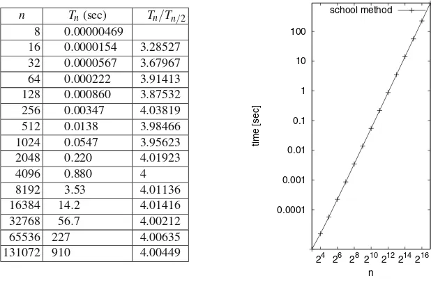
Fig. 1.1.The running time of the school method for the multiplication ofn-digit integers. The three columns of the table on theleftgiven, the running timeTnof the C++implementation given in Sect.1.7, and the ratioTn/Tn/2. The plot on therightshows logTnversus logn, and we see essentially a line. Observe that ifTn=αnβfor some constantsαandβ, thenTn/Tn/2=2β and logTn=βlogn+logα, i.e., logTndepends linearly on lognwith slopeβ. In our case, the slope is two. Please, use a ruler to check

complex transport mechanism for data between memory and the processing unit, but they will have a similar effect for alli, and hence the number of primitive operations is also representative of the running time of an actual implementation on an actual machine. The argument extends to multiplication, since multiplication of a number by a one-digit number is a process similar to addition and the second phase of the school method for multiplication amounts to a series of additions.

Let us confirm the above argument by an experiment. Figure1.1shows execution times of a C++_{implementation of the school method; the program can be found in} Sect.1.7. For each n, we performed a large number4of multiplications of n-digit random integers and then determined the average running timeTn;Tn is listed in the second column. We also show the ratioTn/Tn/2. Figure1.1 also shows a plot of the data points5_(logn,_logT

n). The data exhibits approximately quadratic growth, as we can deduce in various ways. The ratioTn/Tn/2 is always close to four, and the double logarithmic plot shows essentially a line of slope two. The experiments 4_{The internal clock that measures CPU time returns its timings in some units, say} millisec-onds, and hence the rounding required introduces an error of up to one-half of this unit. It is therefore important that the experiment timed takes much longer than this unit, in order to reduce the effect of rounding.

(17)

are quite encouraging:our theoretical analysis has predictive value. Our theoretical analysis showed quadratic growth of the number of primitive operations, we argued above that the running time should be related to the number of primitive operations, and the actual running time essentially grows quadratically.However, we also see systematic deviations. For smalln, the growth from one row to the next is less than by a factor of four, as linear and constant terms in the running time still play a substantial role. For largern, the ratio is very close to four. For very largen(too large to be timed conveniently), we would probably see a factor larger than four, since the access time to memory depends on the size of the data. We shall come back to this point in Sect. 2.2.

Exercise 1.2.Write programs for the addition and multiplication of long integers. Represent integers as sequences (arrays or lists or whatever your programming lan-guage offers) of decimal digits and use the built-in arithmetic to implement the prim-itive operations. Then write ADD, MULTIPLY1, and MULTIPLY functions that add integers, multiply an integer by a one-digit number, and multiply integers, respec-tively. Use your implementation to produce your own version of Fig.1.1. Experiment with using a larger base than base 10, say base 216.

Exercise 1.3.Describe and analyze the school method for division.

1.3 Result Checking

Our algorithms for addition and multiplication are quite simple, and hence it is fair to assume that we can implement them correctly in the programming language of our choice. However, writing software6is an error-prone activity, and hence we should always ask ourselves whether we can check the results of a computation. For multi-plication, the authors were taught the following technique in elementary school. The method is known asNeunerprobe in German, “casting out nines” in English, and preuve par neuf in French.

Add the digits ofa. If the sum is a number with more than one digit, sum its digits. Repeat until you arrive at a one-digit number, called the checksum ofa. We usesato denote this checksum. Here is an example:

4528→19→10→1.

Do the same forb and the resultcof the computation. This gives the checksums s_b andsc. All checksums are single-digit numbers. Compute sa·sb and form its checksums. Ifsdiffers fromsc,cis not equal toa·b. This test was described by al-Khwarizmi in his book on algebra.

(18)

1.4 A Recursive Version of the School Method 7

hencesc is not the product ofa andb. Indeed, the correct product isc=153153. Its checksum is 9, and hence the correct product passes the test. The test is not fool-proof, asc=135153 also passes the test. However, the test is quite useful and detects many mistakes.

What is the mathematics behind this test? We shall explain a more general method. Letqbe any positive integer; in the method described above,q=9. Letsa be the remainder, or residue, in the integer division ofabyq, i.e.,sa=a− ⌊a/q⌋ ·q. Then 0≤sa<q. In mathematical notation,sa=amodq.7Similarly,sb=bmodq andsc=cmodq. Finally,s= (sa·sb)modq. Ifc=a·b, then it must be the case thats=sc. Thuss=scprovesc=a·band uncovers a mistake in the multiplication. What do we know ifs=sc? We know thatq divides the difference ofcanda·b. If this difference is nonzero, the mistake will be detected by anyqwhich does not divide the difference.

Let us continue with our example and takeq=7. Thenamod 7=2,bmod 7=0 and hences= (2·0)mod 7=0. But 135153 mod 7=4, and we have uncovered that 135153=429·357.

Exercise 1.4.Explain why the method learned by the authors in school corresponds to the caseq=9. Hint: 10kmod 9=1 for allk≥0.

Exercise 1.5 (Elferprobe, casting out elevens).Powers of ten have very simple re-mainders modulo 11, namely 10kmod 11= (−1)k_{for all}_k_≥_{0, i.e., 1 mod 11}₌_1, 10 mod 11=−1, 100 mod 11= +1, 1 000 mod 11=−1, etc. Describe a simple test to check the correctness of a multiplication modulo 11.

1.4 A Recursive Version of the School Method

We shall now derive a recursive version of the school method. This will be our first encounter with thedivide-and-conquerparadigm, one of the fundamental paradigms in algorithm design.

Letaandbbe our twon-digit integers which we want to multiply. Letk=⌊n/2⌋. We splitainto two numbersa1anda0;a0consists of thekleast significant digits and a1consists of then−kmost significant digits.8We splitbanalogously. Then

a=a1·Bk+a0 and b=b1·Bk+b0,

and hence

a·b=a1·b1·B2k+ (a1·b0+a0·b1)·Bk+a0·b0. This formula suggests the following algorithm for computinga·b:

7_{The method taught in school uses residues in the range 1 to 9 instead of 0 to 8 according to} the definitionsa=a−(⌈a/q⌉ −1)·q.

8_{Observe that we have changed notation;}_a

(19)

(a) Splitaandbintoa1,a0,b1, andb0.

(b) Compute the four productsa1·b1,a1·b0,a0·b1, anda0·b0. (c) Add the suitably aligned products to obtaina·b.

Observe that the numbersa1,a0,b1, andb0are⌈n/2⌉-digit numbers and hence the multiplications in step (b) are simpler than the original multiplication if⌈n/2⌉<n, i.e.,n>1. The complete algorithm is now as follows. To multiply one-digit numbers, use the multiplication primitive. To multiplyn-digit numbers forn≥2, use the three-step approach above.

It is clear why this approach is calleddivide-and-conquer. We reduce the problem of multiplyinga andbto some number of simplerproblems of the same kind. A divide-and-conquer algorithm always consists of three parts: in the first part, we split the original problem into simpler problems of the same kind (our step (a)); in the second part we solve the simpler problems using the same method (our step (b)); and, in the third part, we obtain the solution to the original problem from the solutions to the subproblems (our step (c)).

. .

a0

a0 a0 a1

a1

a1b0 b0 b0

b1

b1 b1

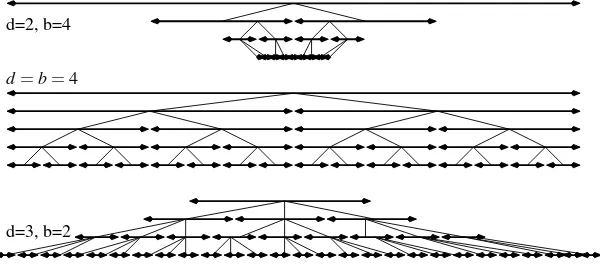
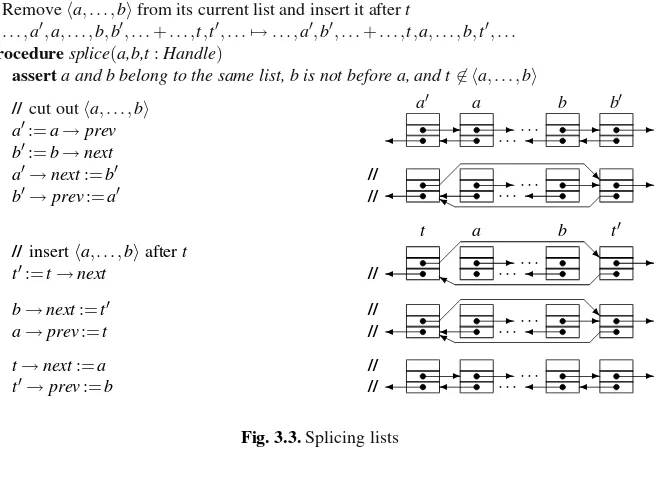
Fig. 1.2.Visualization of the school method and its recursive variant. The rhombus-shaped area indicates the partial products in the multiplication a·b. The four subareas correspond to the partial productsa1·b1,a1·b0,a0·b1, anda0·b0. In the recursive scheme, we first sum the partial prod-ucts in the four subareas and then, in a second step, add the four resulting sums

What is the connection of our recursive integer multiplication to the school method? It is really the same method. Figure 1.2shows that the products a1·b1, a1·b0,a0·b1, anda0·b0are also computed in the school method. Knowing that our recursive integer multiplication is just the school method in disguise tells us that the recursive algorithm uses a quadratic number of primitive operations. Let us also de-rive this from first principles. This will allow us to introduce recurrence relations, a powerful concept for the analysis of recursive algorithms.

Lemma 1.4.Let T(n)be the maximal number of primitive operations required by our recursive multiplication algorithm when applied to n-digit integers. Then

T(n)≤

1 if n=1,

4·T(⌈n/2⌉) +3·2·n if n≥2.

Proof. Multiplying two one-digit numbers requires one primitive multiplication. This justifies the casen=1. So, assumen≥2. Splittingaandbinto the four pieces a1,a0,b1, andb0requires no primitive operations.9Each piece has at most⌈n/2⌉

(20)

1.5 Karatsuba Multiplication 9

digits and hence the four recursive multiplications require at most 4·T(⌈n/2⌉) prim-itive operations. Finally, we need three additions to assemble the final result. Each addition involves two numbers of at most 2ndigits and hence requires at most 2n primitive operations. This justifies the inequality forn≥2. ⊓⊔

In Sect. 2.6, we shall learn that such recurrences are easy to solve and yield the already conjectured quadratic execution time of the recursive algorithm.

Lemma 1.5.Let T(n)be the maximal number of primitive operations required by our recursive multiplication algorithm when applied to n-digit integers. Then T(n)≤ 7n2if n is a power of two, and T(n)≤28n2for all n.

Proof. We refer the reader to Sect.1.8for a proof. ⊓⊔

1.5 Karatsuba Multiplication

In 1962, the Soviet mathematician Karatsuba [104] discovered a faster way of multi-plying large integers. The running time of his algorithm grows likenlog 3≈n1.58. The method is surprisingly simple. Karatsuba observed that a simple algebraic identity al-lows one multiplication to be eliminated in the divide-and-conquer implementation, i.e., one can multiplyn-bit numbers using onlythreemultiplications of integers half the size.

The details are as follows. Letaandbbe our twon-digit integers which we want to multiply. Letk=⌊n/2⌋. As above, we split ainto two numbers a1 anda0; a0 consists of thekleast significant digits anda1consists of then−kmost significant digits. We splitbin the same way. Then

a=a1·Bk+a0 and b=b1·Bk+b0

and hence (the magic is in the second equality)

a·b=a1·b1·B2k+ (a1·b0+a0·b1)·Bk+a0·b0

=a1·b1·B2k+ ((a1+a0)·(b1+b0)−(a1·b1+a0·b0))·Bk+a0·b0.

At first sight, we have only made things more complicated. A second look, how-ever, shows that the last formula can be evaluated with only three multiplications, namely,a1·b1,a1·b0, and(a1+a0)·(b1+b0). We also need six additions.10That is three more than in the recursive implementation of the school method. The key is that additions are cheap compared with multiplications, and hence saving a mul-tiplication more than outweighs three additional additions. We obtain the following algorithm for computinga·b:

(21)

(a) Splitaandbintoa1,a0,b1, andb0. (b) Compute the three products

p2=a1·b1, p0=a0·b0, p1= (a1+a0)·(b1+b0).

(c) Add the suitably aligned products to obtaina·b, i.e., computea·baccording to the formula

a·b=p2·B2k+ (p1−(p2+p0))·Bk+p0.

The numbersa1,a0,b1,b0,a1+a0, and b1+b0are⌈n/2⌉+1-digit numbers and hence the multiplications in step (b) are simpler than the original multiplication if ⌈n/2⌉+1<n, i.e.,n≥4. The complete algorithm is now as follows: to multiply three-digit numbers, use the school method, and to multiplyn-digit numbers forn≥ 4, use the three-step approach above.

10

1

0.1

0.01

0.001

0.0001

1e-05

214 212 210 28 26 24

time [sec]

n school method

Karatsuba4 Karatsuba32

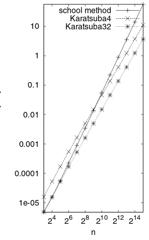
Fig. 1.3.The running times of implemen-tations of the Karatsuba and school meth-ods for integer multiplication. The run-ning times for two versions of Karatsuba’s method are shown: Karatsuba4 switches to the school method for integers with fewer than four digits, and Karatsuba32 switches to the school method for integers with fewer than 32 digits. The slopes of the lines for the Karatsuba variants are approx-imately 1.58. The running time of Karat-suba32 is approximately one-third the run-ning time of Karatsuba4.

Figure1.3shows the running times TK(n)andTS(n)of C++implementations of the Karatsuba method and the school method forn-digit integers. The scales on both axes are logarithmic. We see, essentially, straight lines of different slope. The running time of the school method grows like n2_{, and hence the slope is 2 in the} case of the school method. The slope is smaller in the case of the Karatsuba method and this suggests that its running time grows likenβ withβ <2. In fact, the ratio11 TK(n)/TK(n/2) is close to three, and this suggests thatβ is such that 2β =3 or

11_T

(22)

1.6 Algorithm Engineering 11 β =log 3≈1.58. Alternatively, you may determine the slope from Fig. 1.3. We shall prove below thatTK(n)grows likenlog 3. We say that theKaratsuba method has better asymptotic behavior. We also see that the inputs have to be quite big before the superior asymptotic behavior of the Karatsuba method actually results in a smaller running time. Observe that forn=28_{, the school method is still faster, that for}_n₌₂9_, the two methods have about the same running time, and that the Karatsuba method wins forn=210. The lessons to remember are:

• Better asymptotic behavior ultimately wins.

• An asymptotically slower algorithm can be faster on small inputs.

In the next section, we shall learn how to improve the behavior of the Karatsuba method for small inputs. The resulting algorithm will always be at least as good as the school method. It is time to derive the asymptotics of the Karatsuba method.

Lemma 1.6.Let TK(n)be the maximal number of primitive operations required by the Karatsuba algorithm when applied to n-digit integers. Then

TK(n)≤

3n2+2n if n≤3,

3·TK(⌈n/2⌉+1) +6·2·n if n≥4.

Proof. Multiplying two n-bit numbers using the school method requires no more than 3n2+2nprimitive operations, by Lemma1.3. This justifies the first line. So, assumen≥4. Splittingaandb into the four piecesa1,a0,b1, andb0requires no primitive operations.12 Each piece and the sumsa0+a1andb0+b1have at most ⌈n/2⌉+1 digits, and hence the three recursive multiplications require at most 3· TK(⌈n/2⌉+1)primitive operations. Finally, we need two additions to forma0+a1 andb0+b1, and four additions to assemble the final result. Each addition involves two numbers of at most 2ndigits and hence requires at most 2nprimitive operations.

This justifies the inequality forn≥4. ⊓⊔

In Sect. 2.6, we shall learn some general techniques for solving recurrences of this kind.

Theorem 1.7.Let TK(n)be the maximal number of primitive operations required by the Karatsuba algorithm when applied to n-digit integers. Then TK(n)≤99nlog 3+ 48·n+48·logn for all n.

Proof. We refer the reader to Sect.1.8for a proof. ⊓⊔

1.6 Algorithm Engineering

(23)

digits. However, a simple refinement improves the performance significantly. Since the school method is superior to the Karatsuba method for short integers, we should stop the recursion earlier and switch to the school method for numbers which have fewer than n0 digits for some yet to be determined n0. We call this approach the refined Karatsuba method. It is never worse than either the school method or the original Karatsuba algorithm.

0.4

0.3

0.2

0.1

1024 512 256 128 64 32 16 8 4

recursion threshold Karatsuba, n = 2048 Karatsuba, n = 4096

Fig. 1.4.The running time of the Karat-suba method as a function of the recursion thresholdn0. The times consumed for mul-tiplying 2048-digit and 4096-digit integers are shown. The minimum is atn0=32

What is a good choice forn0? We shall answer this question both experimentally and analytically. Let us discuss the experimental approach first. We simply time the refined Karatsuba algorithm for different values ofn0and then adopt the value giving the smallest running time. For our implementation, the best results were obtained for n0=32 (see Fig.1.4). The asymptotic behavior of the refined Karatsuba method is shown in Fig. 1.3. We see that the running time of the refined method still grows likenlog 3, that the refined method is about three times faster than the basic Karatsuba method and hence the refinement is highly effective, and that the refined method is never slower than the school method.

Exercise 1.6.Derive a recurrence for the worst-case numberTR(n)of primitive op-erations performed by the refined Karatsuba method.

We can also approach the question analytically. If we use the school method to multiplyn-digit numbers, we need 3n2₊_2n _{primitive operations. If we use one} Karatsuba step and then multiply the resulting numbers of length⌈n/2⌉+1 using the school method, we need about 3(3(n/2+1)2₊_2(n/2₊_{1)) +}_12n_primitive op-erations. The latter is smaller forn≥28 and hence a recursive step saves primitive operations as long as the number of digits is more than 28. You should not take this as an indication that an actual implementation should switch at integers of approx-imately 28 digits, as the argument concentrates solely on primitive operations. You should take it as an argument that it is wise to have a nontrivial recursion threshold n0and then determine the threshold experimentally.

(24)

1.7 The Programs 13

more thanα·nmprimitive operations for some constantα. (b) Assumen≥mand divideainto⌈n/m⌉numbers ofmdigits each. Multiply each of the fragments byb using Karatsuba’s method and combine the results. What is the running time of this approach?

1.7 The Programs

We give C++_{programs for the school and Karatsuba methods below. These programs} were used for the timing experiments described in this chapter. The programs were executed on a machine with a 2 GHz dual-core Intel T7200 processor with 4 Mbyte of cache memory and 2 Gbyte of main memory. The programs were compiled with GNU C++_{version 3.3.5 using optimization level}-O2_.

A digit is simply an unsigned int and an integer is a vector of digits; here, “vector” is the vector type of the standard template library. A declarationinteger a(n)declares an integer withndigits,a.size()returns the size ofa, anda[i]returns a reference to the i-th digit ofa. Digits are numbered starting at zero. The global variableBstores the base. The functionsfullAdderanddigitMultimplement the primitive operations on digits. We sometimes need to access digits beyond the size of an integer; the function getDigit(a,i)returnsa[i]ifiis a legal index foraand returns zero otherwise:

typedef unsigned int digit; typedef vector<digit> integer;

unsigned int B = 10; // Base, 2 <= B <= 2^16

void fullAdder(digit a, digit b, digit c, digit& s, digit& carry) { unsigned int sum = a + b + c; carry = sum/B; s = sum - carry*B; }

void digitMult(digit a, digit b, digit& s, digit& carry)

{ unsigned int prod = a*b; carry = prod/B; s = prod - carry*B; }

digit getDigit(const integer& a, int i) { return ( i < a.size()? a[i] : 0 ); }

We want to run our programs on random integers:randDigitis a simple random generator for digits, andrandIntegerfills its argument with random digits.

unsigned int X = 542351;

digit randDigit() { X = 443143*X + 6412431; return X % B ; } void randInteger(integer& a)

{ int n = a.size(); for (int i=0; i<n; i++) a[i] = randDigit();}

(25)

void mult(const integer& a, const digit& b, integer& atimesb) { int n = a.size(); assert(atimesb.size() == n+1);

digit carry = 0, c, d, cprev = 0;

for (int i = 0; i < n; i++) { digitMult(a[i],b,d,c);

fullAdder(d, cprev, carry, atimesb[i], carry); cprev = c; }

d = 0;

fullAdder(d, cprev, carry, atimesb[n], carry); assert(carry == 0);

}

void addAt(integer& p, const integer& atimesbj, int j) { // p has length n+m,

digit carry = 0; int L = p.size(); for (int i = j; i < L; i++)

fullAdder(p[i], getDigit(atimesbj,i-j), carry, p[i], carry); assert(carry == 0);

}

integer mult(const integer& a, const integer& b) { int n = a.size(); int m = b.size();

integer p(n + m,0); integer atimesbj(n+1);

for (int j = 0; j < m; j++)

{ mult(a, b[j], atimesbj); addAt(p, atimesbj, j); } return p;

}

For Karatsuba’s method, we also need algorithms for general addition and sub-traction. The subtraction method may assume that the first argument is no smaller than the second. It computes its result in the first argument:

integer add(const integer& a, const integer& b) { int n = max(a.size(),b.size());

integer s(n+1); digit carry = 0; for (int i = 0; i < n; i++)

fullAdder(getDigit(a,i), getDigit(b,i), carry, s[i], carry); s[n] = carry;

return s; }

void sub(integer& a, const integer& b) // requires a >= b { digit carry = 0;

for (int i = 0; i < a.size(); i++) if ( a[i] >= ( getDigit(b,i) + carry ))

{ a[i] = a[i] - getDigit(b,i) - carry; carry = 0; }

else { a[i] = a[i] + B - getDigit(b,i) - carry; carry = 1;} assert(carry == 0);

}

The functionsplitsplits an integer into two integers of half the size:

void split(const integer& a,integer& a1, integer& a0)

{ int n = a.size(); int k = n/2;

(26)

1.7 The Programs 15

The functionKaratsubaworks exactly as described in the text. If the inputs have fewer thann0digits, the school method is employed. Otherwise, the inputs are split into numbers of half the size and the productsp0,p1, andp2are formed. Thenp0and p2are written into the output vector and subtracted fromp1. Finally, the modifiedp1 is added to the result:

integer Karatsuba(const integer& a, const integer& b, int n0)

{ int n = a.size(); int m = b.size(); assert(n == m); assert(n0 >= 4); integer p(2*n);

if (n < n0) return mult(a,b);

int k = n/2; integer a0(k), a1(n - k), b0(k), b1(n - k);

split(a,a1,a0); split(b,b1,b0);

integer p2 = Karatsuba(a1,b1,n0),

p1 = Karatsuba(add(a1,a0),add(b1,b0),n0), p0 = Karatsuba(a0,b0,n0);

for (int i = 0; i < 2*k; i++) p[i] = p0[i];

for (int i = 2*k; i < n+m; i++) p[i] = p2[i - 2*k];

sub(p1,p0); sub(p1,p2); addAt(p,p1,k);

return p; }

The following program generated the data for Fig.1.3:

inline double cpuTime() { return double(clock())/CLOCKS_PER_SEC; }

int main(){

for (int n = 8; n <= 131072; n *= 2)

{ integer a(n), b(n); randInteger(a); randInteger(b);

double T = cpuTime(); int k = 0;

while (cpuTime() - T < 1) { mult(a,b); k++; }

cout << "\n" << n << " school = " << (cpuTime() - T)/k;

T = cpuTime(); k = 0;

while (cpuTime() - T < 1) { Karatsuba(a,b,4); k++; }

cout << " Karatsuba4 = " << (cpuTime() - T) /k; cout.flush();

T = cpuTime(); k = 0;

while (cpuTime() - T < 1) { Karatsuba(a,b,32); k++; }

cout << " Karatsuba32 = " << (cpuTime() - T) /k; cout.flush(); }

(27)

1.8 Proofs of Lemma

1.5

and Theorem

1.7

To make this chapter self-contained, we include proofs of Lemma 1.5 and Theo-rem 1.7. We start with an analysis of the recursive version of the school method. Recall thatT(n), the maximal number of primitive operations required by our recur-sive multiplication algorithm when applied ton-digit integers, satisfies

T(n)≤

1 ifn=1,

4·T(⌈n/2⌉) +3·2·n ifn≥2.

We use induction onnto show thatT(n)≤7n2−6nwhennis a power of two. For n=1, we haveT(1)≤1=7n2−6n. Forn>1, we have

T(n)≤4T(n/2) +6n≤4(7(n/2)2−6n/2) +6n=7n2−6n,

where the second inequality follows from the induction hypothesis. For generaln, we observe that multiplyingn-digit integers is certainly no more costly than multiplying 2⌈logn⌉-digit integers and henceT(n)≤T(2⌈logn⌉_{). Since 2}⌈logn⌉_≤_{2n, we conclude} thatT(n)≤28n2for alln.

Exercise 1.8.Prove a bound on the recurrenceT(1)≤1 andT(n)≤4T(n/2) +9n whennis a power of two.

How did we know that “7n2−6n” was the bound to be proved? There is no magic here. Forn=2k, repeated substitution yields

T(2k)≤4·T(2k−1) +6·2k≤42T(2k−2) +6·(41·2k−1+2k) ≤43T(2k−3) +6·(42·2k−2+41·2k−1+2k)≤. . . ≤4kT(1) +6

∑

0≤i≤k−1

4i2k−i≤4k+6·2k

∑

0≤i≤k−1

2i

≤4k+6·2k(2k₋_{1) =}_n2₊_6n(n₋_{1) =}_7n2₋_6n_.

We turn now to the proof of Theorem1.7. Recall thatTKsatisfies the recurrence

TK(n)≤

3n2+2n ifn≤3,

3·TK(⌈n/2⌉+1) +12n ifn≥4.

The recurrence for the school method has the nice property that ifnis a power of two, the arguments ofT on the right-hand side are again powers of two. This is not true forTK. However, ifn=2k+2 andk≥1, then⌈n/2⌉+1=2k−1+2, and hence we should now use numbers of the formn=2k+2,k≥0, as the basis of the inductive argument. We shall show that

(28)

1.9 Implementation Notes 17

TK(20+2) =TK(3)≤3·32+2·3=33=33·20+12·(21+2·0−2).

Fork≥1, we have

TK(2k+2)≤3TK(2k−1+2) +12·(2k+2)

≤3·33·3k−1+12·(2k+2(k−1)−2)+12·(2k+2) =33·3k+12·(2k+1₊_2k₋₂₎_.

Again, there is no magic in coming up with the right induction hypothesis. It is obtained by repeated substitution. Namely,

TK(2k+2)≤3TK(2k−1+2) +12·(2k+2)

≤3kTK(20+2) +12·(2k+2+2k−1+2+. . .+21+2) ≤33·3k+12·(2k+1₋₂₊_2k)_.

It remains to extend the bound to all n. Let k be the minimal integer such that n≤2k+2. Thenk≤1+logn. Also, multiplyingn-digit numbers is no more costly than multiplying(2k_{+2)-digit numbers, and hence}

TK(n)≤33·3k+12·(2k+1−2+2k)

≤99·3logn+48·(2logn₋₂₊₂₍₁_+log_n)) ≤99·nlog 3+48·n+48·logn,

where the equality 3logn=2(log 3)·(logn)=nlog 3has been used. Exercise 1.9.Solve the recurrence

TR(n)≤

3n2+2n ifn<32, 3·TR(⌈n/2⌉+1) +12n ifn≥4.

1.9 Implementation Notes

The programs given in Sect.1.7are not optimized. The base of the number system should be a power of two so that sums and carries can be extracted by bit operations. Also, the size of a digit should agree with the word size of the machine and a little more work should be invested in implementing primitive operations on digits.

1.9.1 C++

(29)

1.9.2 Java

java.mathimplements arbitrary-precision integers and floating-point numbers.

1.10 Historical Notes and Further Findings

Is the Karatsuba method the fastest known method for integer multiplication? No, much faster methods are known. Karatsuba’s method splits an integer into two parts and requires three multiplications of integers of half the length. The natural exten-sion is to split integers intokparts of lengthn/keach. If the recursive step requiresℓ multiplications of numbers of lengthn/k, the running time of the resulting algorithm grows likenlogkℓ_{. In this way, Toom [196] and Cook [43] reduced the running time} to13On1+εfor arbitrary positiveε. The asymptotically most efficient algorithms are the work of Schönhage and Strassen [171] and Schönhage [170]. The former multipliesn-bit integers with O(nlognlog logn)bit operations, and it can be imple-mented to run in this time bound on a Turing machine. The latter runs in linear time O(n)and requires the machine model discussed in Sect. 2.2. In this model, integers with lognbits can be multiplied in constant time.

(30)

2

Introduction

When you want to become a sculptor1 you have to learn some basic techniques: where to get the right stones, how to move them, how to handle the chisel, how to erect scaffolding, . . . . Knowing these techniques will not make you a famous artist, but even if you have a really exceptional talent, it will be very difficult to develop into a successful artist without knowing them. It is not necessary to master all of the basic techniques before sculpting the first piece. But you always have to be willing to go back to improve your basic techniques.

This introductory chapter plays a similar role in this book. We introduce basic concepts that make it simpler to discuss and analyze algorithms in the subsequent chapters. There is no need for you to read this chapter from beginning to end before you proceed to later chapters. On first reading, we recommend that you should read carefully to the end of Sect.2.3and skim through the remaining sections. We begin in Sect.2.1by introducing some notation and terminology that allow us to argue about the complexity of algorithms in a concise way. We then introduce a simple machine model in Sect.2.2that allows us to abstract from the highly variable complications introduced by real hardware. The model is concrete enough to have predictive value and abstract enough to allow elegant arguments. Section2.3then introduces a high-level pseudocode notation for algorithms that is much more convenient for express-ing algorithms than the machine code of our abstract machine. Pseudocode is also more convenient than actual programming languages, since we can use high-level concepts borrowed from mathematics without having to worry about exactly how they can be compiled to run on actual hardware. We frequently annotate programs to make algorithms more readable and easier to prove correct. This is the subject of Sect.2.4. Section2.5gives the first comprehensive example: binary search in a sorted array. In Sect.2.6, we introduce mathematical techniques for analyzing the complexity of programs, in particular, for analyzing nested loops and recursive

(31)

cedure calls. Additional analysis techniques are needed for average-case analysis; these are covered in Sect.2.7. Randomized algorithms, discussed in Sect.2.8, use coin tosses in their execution. Section2.9is devoted to graphs, a concept that will play an important role throughout the book. In Sect.2.10, we discuss the question of when an algorithm should be called efficient, and introduce the complexity classes PandNP. Finally, as in every chapter of this book, there are sections containing im-plementation notes (Sect.2.11) and historical notes and further findings (Sect.2.12).

2.1 Asymptotic Notation

The main purpose of algorithm analysis is to give performance guarantees, for ex-ample bounds on running time, that are at the same time accurate, concise, general, and easy to understand. It is difficult to meet all these criteria simultaneously. For example, the most accurate way to characterize the running timeT of an algorithm is to viewT as a mapping from the setIof all inputs to the set of nonnegative numbers R+. For any problem instancei,T(i)is the running time oni. This level of detail is so overwhelming that we could not possibly derive a theory about it. A useful theory needs a more global view of the performance of an algorithm.

We group the set of all inputs into classes of “similar” inputs and summarize the performance on all instances in the same class into a single number. The most useful grouping is bysize. Usually, there is a natural way to assign a size to each problem instance. The size of an integer is the number of digits in its representation, and the size of a set is the number of elements in the set. The size of an instance is always a natural number. Sometimes we use more than one parameter to measure the size of an instance; for example, it is customary to measure the size of a graph by its number of nodes and its number of edges. We ignore this complication for now. We use size(i)to denote the size of instancei, andInto denote the instances of sizen forn_∈N. For the inputs of sizen, we are interested in the maximum, minimum, and average execution times:2

worst case: T(n) =max{T(i):i_∈In} best case: T(n) =min{T(i):i_∈In}

average case: T(n) = 1 |In|_i

∑

_∈_In

T(i).

We are interested most in the worst-case execution time, since it gives us the strongest performance guarantee. A comparison of the best case and the worst case tells us how much the execution time varies for different inputs in the same class. If the discrepancy is big, the average case may give more insight into the true perfor-mance of the algorithm. Section2.7gives an example.

We shall perform one more step of data reduction: we shall concentrate ongrowth rateorasymptotic analysis. Functions f(n)andg(n)have thesame growth rateif

2_{We shall make sure that}_{_T_(i)_:_i_∈_I

(32)

2.1 Asymptotic Notation 21

there are positive constantscandd such thatc_≤ f(n)/g(n)≤d for all sufficiently largen, and f(n) grows fasterthan g(n)if, for all positive constants c, we have f(n)≥c_·g(n)for all sufficiently largen. For example, the functionsn2,n2+7n, 5n2₋_{7n, and}_n2_/₁₀₊₁₀6_n _{all have the same growth rate. Also, they grow faster} thann3/2_{, which in turn grows faster than}_n_log_{n. The growth rate talks about the} behavior for largen. The word “asymptotic” in “asymptotic analysis” also stresses the fact that we are interested in the behavior for largen.

Why are we interested only in growth rates and the behavior for largen? We are interested in the behavior for largenbecause the whole purpose of designing efficient algorithms is to be able to solve large instances. For largen, an algorithm whose running time has a smaller growth rate than the running time of another algorithm will be superior. Also, our machine model is an abstraction of real machines and hence can predict actual running times only up to a constant factor, and this suggests that we should not distinguish between algorithms whose running times have the same growth rate. A pleasing side effect of concentrating on growth rate is that we can characterize the running times of algorithms by simple functions. However, in the sections on implementation, we shall frequently take a closer look and go beyond asymptotic analysis. Also, when using one of the algorithms described in this book, you should always ask yourself whether the asymptotic view is justified.

The following definitions allow us to argue precisely aboutasymptotic behavior. Letf(n)andg(n)denote functions that map nonnegative integers to nonnegative real numbers:

O(f(n)) ={g(n):∃c>0 :∃n0∈N+:∀n≥n0:g(n)≤c·f(n)}, Ω(f(n)) ={g(n):_∃c>0 :_∃n0∈N+:∀n≥n0:g(n)≥c·f(n)}, Θ(f(n)) =O(f(n))∩Ω(f(n)),

o(f(n)) ={g(n):∀c>0 :∃n0∈N+:∀n≥n0:g(n)≤c·f(n)}, ω(f(n)) ={g(n):∀c>0 :∃n0∈N+:∀n≥n0:g(n)≥c·f(n)}.

The left-hand sides should be read as “big O of f”, “big omega of f”, “theta of f”, “little o of f”, and “little omega of f”, respectively.

Let us see some examples. O

n2is the set of all functions that grow at most quadratically, o

n2

is the set of functions that grow less than quadratically, and o(1) is the set of functions that go to zero asn goes to infinity. Here “1” stands for the functionn_→1, which is one everywhere, and hence f _∈o(1) if f(n)≤

c_·1 for any positivecand sufficiently largen, i.e., f(n)goes to zero asn goes to infinity. Generally, O(f(n))is the set of all functions that “grow no faster than” f(n). Similarly,Ω(f(n))is the set of all functions that “grow at least as fast as” f(n). For example, the Karatsuba algorithm for integer multiplication has a worst-case running time in On1.58, whereas the school algorithm has a worst-case running time in Ω

n2

(33)

The growth rate of most algorithms discussed in this book is either a polynomial or a logarithmic function, or the product of a polynomial and a logarithmic func-tion. We use polynomials to introduce our readers to some basic manipulations of asymptotic notation.

Lemma 2.1.Let p(n) =∑ki=0ainidenote any polynomial and assume ak>0. Then p(n)∈Θ

nk.

Proof. It suffices to show thatp(n)∈Onkandp(n)∈Ω

nk. First observe that for n>0,

p(n)≤

k

∑

i=0

|ai|ni≤nk k

∑

i=0

|ai|,

and hencep(n)≤(∑ki=0|ai|)nkfor all positiven. Thus p(n)∈O

nk. LetA=∑k_i=0−1|ai|. For positivenwe have

p(n)≥aknk−Ank−1= a_k

2n

k₊_nk−1ak 2n−A

and hence p(n)≥(ak/2)nkforn>2A/ak. We choosec=ak/2 andn0=2A/akin the definition ofΩ

nk

, and obtainp(n)∈Ω

nk

. ⊓⊔

Exercise 2.1.Right or wrong? (a)n2+106n_∈O

n2

, (b)nlogn_∈O(n), (c)nlogn∈

Ω(n), (d) logn∈o(n).

Asymptotic notation is used a lot in algorithm analysis, and it is convenient to stretch mathematical notation a little in order to allow sets of functions (such as O

n2

) to be treated similarly to ordinary functions. In particular, we shall always writeh=O(f)instead ofh_∈O(f), and O(h) =O(f)instead of O(h)⊆O(f). For example,

3n2+7n=O

n2 =O

n3

.

Be warned that sequences of equalities involving O-notation should only be read from left to right.

Ifh is a function,F andGare sets of functions, and◦ is an operator such as

+,·, or/, thenF_◦Gis a shorthand for{f_◦g:f _∈F,g_∈G_}, andh_◦F stands for

{h_{} ◦}F. So f(n) +o(f(n))denotes the set of all functions f(n) +g(n)whereg(n)

grows strictly more slowly than f(n), i.e., the ratio(f(n) +g(n))/f(n)goes to one asngoes to infinity. Equivalently, we can write(1+o(1))f(n). We use this notation whenever we care about the constant in the leading term but want to ignore lower-order terms.

Lemma 2.2.The following rules hold forO-notation:

c f(n) =Θ(f(n))for any positive constant,

f(n) +g(n) =Ω(f(n)),

f(n) +g(n) =O(f(n))if g(n) =O(f(n)),

(34)

2.2 The Machine Model 23

Exercise 2.2.Prove Lemma2.2.

Exercise 2.3.Sharpen Lemma2.1and show thatp(n) =aknk+onk.

Exercise 2.4.Prove thatnk=o(cn)for any integerkand anyc>1. How doesnlog logn compare withnkandcn?

2.2 The Machine Model

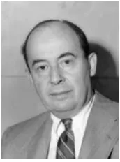
Fig. 2.1. John von Neumann born Dec. 28, 1903 in Budapest, died Feb. 8, 1957 in Washing-ton, DC

In 1945, John von Neumann (Fig.2.1) introduced a computer architecture [201] which was simple, yet powerful. The limited hardware technology of the time forced him to come up with an elegant de-sign that concentrated on the essentials; otherwise, realization would have been impossible. Hardware technology has developed tremendously since 1945. However, the programming model resulting from von Neumann’s design is so elegant and powerful that it is still the basis for most of modern programming. Usu-ally, programs written with von Neumann’s model in mind also work well on the vastly more complex hardware of today’s machines.

The variant of von Neumann’s model used in al-gorithmic analysis is called theRAM(random access machine) model. It was introduced by Sheperdson and Sturgis [179]. It is asequentialmachine with uni-form memory, i.e., there is a single processing unit, and all memory accesses take the same amount of

time. The memory or store, consists of infinitely many cells S[0], S[1], S[2], . . . ; at any point in time, only a finite number of them will be in use.

(35)

Our model supports a limited form of parallelism. We can perform simple operations on a logarithmic number of bits in constant time.

In addition to the main memory, there are a small number ofregisters R1, . . . ,Rk. Our RAM can execute the followingmachine instructions:

• Ri:=S[Rj]loadsthe contents of the memory cell indexed by the contents ofRj into registerRi.

• S[Rj]:=RistoresregisterRiinto the memory cell indexed by the contents ofRj.

• Ri:=Rj⊙Rℓis a binary register operation where “⊙” is a placeholder for a va-riety of operations. Thearithmeticoperations are the usual+,−, and∗but also the bitwise operations|(OR),&(AND),>>(shift right),<<(shift left), and⊕

(exclusive OR, XOR). The operationsdivandmodstand for integer division and the remainder, respectively. The comparisonoperations ≤,<,>, and≥yield true( = 1) orfalse( = 0). Thelogicaloperations∧and∨manipulate thetruth values0 and 1. We may also assume that there are operations which interpret the bits stored in a register as a floating-point number, i.e., a finite-precision approx-imation of a real number.

• Ri:=⊙Rj is a unary operation using the operators−,¬ (logical NOT), or ~ (bitwise NOT).

• Ri:=Cassigns aconstantvalue toRi.

• JZ _j_,_R_i_{continues execution at memory address} _j_{if register}_R_i_{is zero.} • J _j_{continues execution at memory address} _j.

Each instruction takes one time step to execute. The total execution time of a program is the number of instructions executed. A program is a list of instructions numbered starting at one. The addresses in jump-instructions refer to this numbering. The input for a computation is stored in memory cellsS[1]toS[R1].

It is important to remember that the RAM model is an abstraction. One should not confuse it with physically existing machines. In particular, real machines have a finite memory and a fixed number of bits per register (e.g., 32 or 64). In contrast, the word size and memory of a RAM scale with input size. This can be viewed as an abstraction of the historical development. Microprocessors have had words of 4, 8, 16, and 32 bits in succession, and now often have 64-bit words. Words of 64 bits can index a memory of size 264_{. Thus, at current prices, memory size is limited by} cost and not by physical limitations. Observe that this statement was also true when 32-bit words were introduced.

(36)

2.2 The Machine Model 25

We could attempt to introduce a very accurate cost model, but this would miss the point. We would end up with a complex model that would be difficult to handle. Even a successful complexity analysis would lead to a monstrous formula depending on many parameters that change with every new processor generation. Although such a formula would contain detailed information, the very complexity of the formula would make it useless. We therefore go to the other extreme and eliminate all model parameters by assuming that each instruction takes exactly one unit of time. The result is that constant factors in our model are quite meaningless – one more reason to stick to asymptotic analysis most of the time. We compensate for this drawback by providing implementation notes, in which we discuss implementation choices and trade-offs.

2.2.1 External Memory

The biggest difference between a RAM and a real machine is in the memory: a uniform memory in a RAM and a complex memory hierarchy in a real machine. In Sects. 5.7, 6.3, and 7.6, we shall discuss algorithms that have been specifically designed for huge data sets which have to be stored on slow memory, such as disks. We shall use theexternal-memory modelto study these algorithms.

The external-memory model is like the RAM model except that the fast memory Sis limited in size toM words. Additionally, there is an external memory with un-limited size. There are specialI/O operations, which transferBconsecutive words between slow and fast memory. For example, the external memory could be a hard disk,M would then be the size of the main memory, andBwould be a block size that is a good compromise between low latency and high bandwidth. With current technology,M=2 Gbyte andB=2 Mbyte are realistic values. One I/O step would then take around 10 ms which is 2·107_{clock cycles of a 2 GHz machine. With} an-other setting of the parametersM andB, we could model the smaller access time difference between a hardware cache and main memory.

2.2.2 Parallel Processing

(37)

of parallelism. We shall therefore restrict ourselves to occasional informal arguments as to why a certain sequential algorithm may be more or less easy to adapt to paral-lel processing. For example, the algorithms for high-precision arithmetic in Chap. 1 could make use of SIMD instructions.

2.3 Pseudocode

Our RAM model is an abstraction and simplification of the machine programs exe-cuted on microprocessors. The purpose of the model is to provide a precise definition of running time. However, the model is much too low-level for formulating complex algorithms. Our programs would become too long and too hard to read. Instead, we formulate our algorithms inpseudocode, which is an abstraction and simplification of imperative programming languages such as C, C++, Java, C#, and Pascal, combined with liberal use of mathematical notation. We now describe the conventions used in this book, and derive a timing model for pseudocode programs. The timing model is quite simple:basic pseudocode instructions take constant time, and procedure and function calls take constant time plus the time to execute their body. We justify the timing model by outlining how pseudocode can be translated into equivalent RAM code. We do this only to the extent necessary to understand the timing model. There is no need to worry about compiler optimization techniques, since constant factors are outside our theory. The reader may decide to skip the paragraphs describing the translation and adopt the timing model as an axiom. The syntax of our pseudocode is akin to that of Pascal [99], because we find this notation typographically nicer for a book than the more widely known syntax of C and its descendants C++and Java.

2.3.1 Variables and Elementary Data Types

Avariable declaration“v=x :T” introduces a variablevof typeT, and initializes it with the valuex. For example, “answer= 42 :N” introduces a variableanswer assuming integer values and initializes it to the value 42. When the type of a