Evaluation of the uncertainty of groundw

(1)

Evaluation of the uncertainty of groundwater model

predictions associated with conceptual errors: A per-datum

approach to model calibration

Petros Gaganis

a,*

, Leslie Smith

b

a_{Department of the Environment, University of the Aegean, University Hill, Xenia Building, 81100 Mytilene, Greece} b_{Department of Earth and Ocean Sciences, University of British Columbia, V6T 1Z4 Vancouver, Canada}

Received 21 January 2005; accepted 20 June 2005 Available online 3 August 2005

Abstract

The effect of systematic model error on the model predictions varies in space and time, and differs for the flow and solute trans-port components of a groundwater model. The classical single-objective formulation of the inverse problem by its nature cannot capture these characteristics of model error. We introduce an inverse approach that allows the spatial and temporal variability of model error to be evaluated in the parameter space. A set of solutions for model parameters are obtained by this new method that almost exactly satisfies the model equation at each observation point (per-datum calibration). This set of parameter estimates are then used to define a posterior parameter space that may be translated into a probabilistic description of model output to rep-resent the level of confidence in model performance. It is shown that this approach can provide useful information regarding the strengths and limitations of a model as well as the performance of classical calibration procedures.

Keywords: Model error; Conceptual error; Predictive uncertainty; Model calibration; Model selection

1. Introduction

There are two types of error associated with mathe-matical modeling of hydrologic systems: (i) parameter errorthat is mainly produced from uncertainties related to defining the effective values of the hydraulic or trans-port parameters of a groundwater model, and (ii)model error(or conceptual error) that results from an incorrect model structure. The parameters of a groundwater model, such as hydraulic conductivity, are always uncertain because of measurement error, heterogeneity, and scal-ing issues (e.g.,[2]). The quantification and propagation of parameter uncertainty has been studied extensively in

the past three decades leading to the development of various stochastic methods for assessing the impact of input parameter uncertainty on model predictions (see [12,13,17,40]). There are at least three important sources of model error. First, mathematical and modeling limi-tations result in all models being simplifications and approximations of reality [34]. This source of model error is related to such issues as the use of one-dimen-sional or two-dimenone-dimen-sional models to describe three-dimensional processes, parameterization scheme, description of heterogeneity, zonation of recharge areas or mapping of source zones at contaminant sites, the assumption of isothermal conditions or steady-state flow, the use of the Fickian model to quantify the disper-sive flux, and the use of a finite domain. Second, the existence of knowledge gaps regarding the natural pro-cesses involved will also lead to uncertainty in model

*

Corresponding author. Tel.: +30 2251036293.

E-mail address:gaganis@aegean.gr(P. Gaganis).

(2)

prediction. An example of this source of model error is the representation of multiple processes as a single pro-cess when there is little information on their mathemat-ical description. The mathematmathemat-ical definition of such processes is often empirical and speculative. The release function of contaminants into a flow system can be also cited as an example. The source concentration and its temporal and spatial distribution can be the result of complex serial or parallel processes. Such processes may involve mechanical and chemical weathering, bio-chemical and biological influences on the form of each component, infiltration and dissolution rates, and flow and transport through the unsaturated zone. Detailed modeling of all these processes is practically impossible. Third, our inability to predict how physical or chemical characteristics of the hydrogeological system might change in the future will give rise to additional uncer-tainty. In the common practice of extrapolating from the past to the future, there is not only uncertainty from the imperfect description of the past, but also uncer-tainty about how much the future will be like the past [27]. Model error arising from sources one and two can be reduced with further research and more detailed modeling. However, the third source of model error should be distinguished from the other two as being irre-ducible even in principle. This source of error defines the limits of prediction reliability when modeling physical systems.

The development of a simulation model to aid in the solution of a groundwater problem can be broadly viewed as a procedure that includes four sequential steps: (1) model construction, (2) model calibration, (3) model selection from among alternative calibrated models, which in a sense is equivalent to model valida-tion, and (4) model prediction of system behavior under changed conditions or in the future. Step 1 begins with the formulation of an appropriate conceptual model, which is then translated into a mathematical model. In step 2 and step 3, the appropriate conceptual model and parameter values are selected by minimizing the model misfit to field data through an iterative (inverse) exercise. There are several criteria suggested during the last three decades for selecting among alternative con-ceptual models (e.g., [11,6,24,30,32]) or combinations of several model structures and parameters sets [3,29,39]. More detail on the main model selection meth-odologies as well as their strengths and limitations can be found in [16]. For a review and comparison of the most important approaches to model calibration the reader is referred to [5,26,41]. Typically, the goodness of fit between model output and field data is used as a measure for judging not only the performance of model calibration and model selection but also the effectiveness of the selected model as a predictive tool (step 4). How-ever, the primary goal of a groundwater modeling exer-cise is to obtain reliable model predictions, ideally in the

form of a probability distribution for the dependent variables such as hydraulic head and/or solute concen-tration to be used, for example, in a decision process. Hydrogeological decision models provide a framework to take explicit account of the uncertainty in model pre-dictions during the evaluation of different management alternatives (e.g.,[15,33]). Typically, the more informa-tive the probability distribution for the dependent vari-able (i.e. the model prediction), the more likely it is that a clear and unequivocal determination of the pre-ferred management alternative will be achieved. Model calibration and model selection (step 2 and step 3) rep-resent the means to this goal. Although there have been a number of successes in applying mathematical models in such hydrologic problems, failure or inconsistency of such applications is not uncommon [4]. Application of model selection and model calibration methodologies may not necessarily justify high confidence in the predic-tive capability of a groundwater model. This point is illustrated with several case histories in [4,23]. It is fur-ther argued in [34]that, when a complex hydrogeologic system is described by a simplified numerical model, it is more likely that errors in the model structure represent a main cause of failure of a model application. In such applications, it is critical that the use of a simulation model in predictive modeling (step 4), be accompanied by a realistic evaluation of prediction uncertainty associ-ated not only with parameter error (due to uncertainty in parameter values) but also with errors in the structure of the model itself[16,21].

Model error and parameter uncertainty are interre-lated. The quantiﬁcation of model error is a prerequisite for a meaningful analysis of parameter uncertainty. Alternatively, parameter uncertainty, which is large in most hydrogeologic problems, obscures the impact of model error on model predictions[16]. It is our view that an approach that could lead to distinguishing model error from parameter error should address the reduction of parameter uncertainty and be based on realistic assumptions regarding the statistical characteristics of model error. There are two ways to reduce parameter uncertainty in a modeling exercise: (i) by model calibra-tion, which brings in all the information on the param-eters that is embedded in a set of measurements of the dependent variables, and (ii) by reducing the size of the prior parameter spaceH_{(i.e. region in the parameter}

space that contains all possible combinations of feasible parameter values) with more measurements on the real system. The evaluation of model error by means of updating the prior parameter spaceH_{through collection}

(3)

inverse procedures, to extract useful information on er-rors in model structure from the data and to project their effect onto model predictions. The potential advan-tage of such a methodology is that it would provide the means for assessing the prediction uncertainty associ-ated not only with parameter uncertainty, but also with errors in the structure of a model and it would offer a more informative picture of the real hydrologic situation for decision making. An application of both the Bayes-ian framework and this model calibration approach to a real world pollution problem and decision analysis that explores the utility, and the conceptual and philosophi-cal differences between the two approaches will be pre-sented in a forthcoming publication.

2. A synthetic example

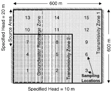
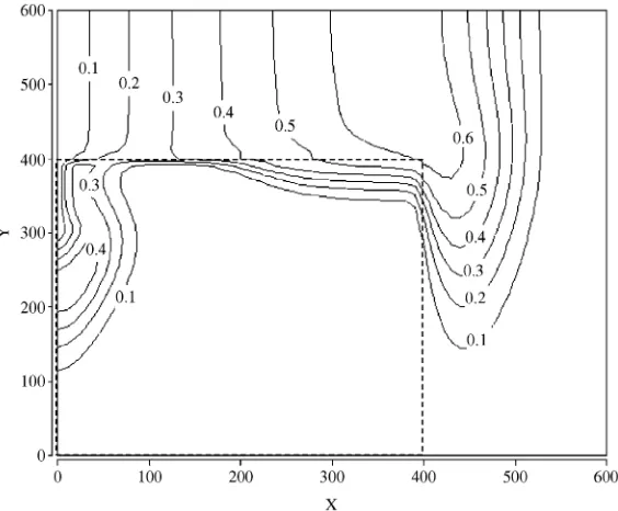
To illustrate our approach a simple two-dimensional synthetic flow system is constructed (model 1). This flow problem was also used in [16]. The flow system is 600 m·_{600 m and contains two homogeneous and} isotropic transmissivity zones, one zone of enhanced recharge and two specified head boundaries (Fig. 1). The rest of the model boundaries are no flow bound-aries. The flow system is assumed to be at steady state. For the contaminant transport problem, solute is intro-duced at the source area along the upstream constant head boundary. Hydraulic heads and solute concentra-tions are measured at 15 sampling locaconcentra-tions equally dis-tributed throughout the flow domain. Observed (free of measurement error) values of hydraulic heads and solute concentrations are simulated by running a forward deterministic simulation using the true parameter values shown inTable 1, and calculating them at the 15 sam-pling locations. The true contaminant release function is assumed to be linear between a normalized concentra-tion value equal to 1 at time zero and 0 at 500 days. The true concentration distribution for the synthetic example

at time 500 days is shown inFig. 2. Adding Gaussian er-rors to the simulated true observations with a standard deviation of 10 cm for the hydraulic head and 5.0% of the concentration values generated the observed data values, subject to measurement error.

Two other models are constructed by introducing model error to the true model described above. Model 2 assumes a uniform contaminant source release func-tion. A constant contaminant concentration equal to 1 is introduced into the system for 250 days. The source duration is designed to introduce the same solute mass into the system as that of the true model. Only the solu-tion of the transport problem of model 2 is influenced by the model error, the flow problem is not. In model 3, the recharge area is expanded in the horizontal direction from 200 m to 300 m. This increase in recharge will affect both the flow and the solute transport parts of the problem. The true linear source function is used in model 3. For all models, only the two transmissivities are considered uncertain and are estimated.

Prior information on the effective values of the two transmissivity zones is incorporated into our analysis by defining a range of feasible parameter values (prior parameter space) within the parameter space of the model (Table 2). For the given example problem, our analysis is not sensitive to the adoption of a greater prior parameter space. Therefore, a relatively small parameter range is assigned to the uncertain parameters to reduce the computational cost. The prior parameter distribu-tions are assumed uniform. It is realistic that, even when prior information is limited, we can usually specify upper and lower bounds to constrain the prior parame-ter space. Although there may be more appropriate ways to include prior information in inverse procedures (e.g., [6,7,9,10]), this way (specified bounds) is adopted here primarily for demonstration reasons.

3. Quantification of model error via inversion

The forward problem that describes the relation be-tween the values of a dependent variable observed in

Fig. 1. True geometry and boundary conditions of the synthetic ﬂow model.

Table 1

True parameter values in deterministic simulation

Parameter Value

Recharge (m/day) 0.0004

Porosity

Transmissivity zone 1 0.2

Transmissivity zone 2 0.2

Transmissivity (m2_/day)

Transmissivity zone 1 20

Transmissivity zone 2 2

Dispersivity (both zones) (m)

Longitudinal 10

(4)

the ﬁeld and model predictions may be represented with an equation in the following form:

d¼fðh_{Þ þ}_Er_ðh_Þ _ð₁_Þ

wheredandh_{are the vectors of observations and model}

parameters respectively,fis the forward equation repre-senting the mathematical model and the vectorEr(h_{) is}

a residual which describes the deviation between mea-sured and predicted values of the dependent variables. Vector h _{includes all uncertain model parameters that}

describe properties of the physical system or their asso-ciated spatial variability. Each component of Er(h₎

ac-counts for measurement error eoj as well as for model

imperfections [erj(h) =eoj+emj], whereemjis the model

error and j= 1,. . .,mis the number of available obser-vations of the dependent variable. In groundwater hydrology the forward equation is typically the ground-water ﬂow or/and advection–dispersion equations, subject to initial and boundary conditions. Inverse pro-cedures deﬁne an inverse estimator fthat connects the observationsdto ‘‘good’’ estimates^h_{of the parameters}

of interest:

^

h_¼_f_½_f_ðh_{Þ þ}_Er_ðh_Þ _ð₂_Þ

The approach that is traditionally used to solve this problem is the classical single-objective formulation of the inverse problem. In the single-objective formulation of the inverse problem, a solution (the parameter vector

^

h_{) is typically obtained by (i) making some assumptions}

regarding the statistical distribution oferj(h), (ii)

apply-ing maximum likelihood or Bayesian theory to construct an objective function that computes some weighted sum of the residual quantities erj(h), and (iii) optimizing this

function (minimizing the measure of residual sum) with respect toh_{in such a way that the distribution of model}

output residual approximates the assumed error statisti-cal distributions. A second objective, that of physistatisti-cal plausibility, may also be included to the objective func-tion by adding to the terms that penalize deviafunc-tions of predictions from observations a second term that penal-izes deviations of estimated parameter values from prior parameter estimates (e.g.,[6,7,9,10,22,28]). A review and comparison of the most important inverse methods the reader can be found in[5,26,41]. A detailed set of guide-lines for the eﬀective calibration of groundwater models is presented in[20]. For joint parameter estimation using hydraulic heads, solute concentrations and prior infor-mation on the parameters, a general form of the sin-gle-objective optimization problem is:

minðwith respect to h_{Þ ½ð}_dh_fh_ðh_ÞÞT_V1

h ðdhfhðhÞÞ

þ ðdcfcðhÞÞTVc1ðdcfcðhÞÞ

þ ðh_ph_ÞT_V1

p ðhphÞ ð3Þ

where the subscripts h and c denote those terms relating to hydraulic head data and solute concentration data respectively, and the subscript ÔpÕ denotes the terms

Fig. 2. True concentration distribution at 500 days.

Table 2

Prior distributions assigned to uncertain parameters

Parameter Distribution Lower

bound

Mean Upper

bound

Transmissivity (m2_/day)

Zone 1 Uniform 10 20 30

(5)

relating to prior information. MatricesVhandVcdeﬁne the covariances among the hydraulic head and concen-tration data respectively, and the matrixVp represents the accuracy of prior information and weights the third term against the ﬁrst two. Once the ‘‘best’’ parameter estimates ^h _{are computed using an objective function}

like(3), they may be used in the forward equationf(h₎

to calculate the model prediction of the dependent vari-able(s). Prediction uncertainty may be also quantiﬁed using either linear or non-linear approximations, or Monte Carlo methods[5]. The magnitude of prediction uncertainty is related to the parameter estimation error which is, in turn, related to parameter sensitivity and to the standard error of the inverse procedure (value of the objective function(3))[20,26]. The ‘‘size’’ of these errors is often measured in terms of their variances or covariance matrices.

In the case that model error is small or somehow ab-sorbed into the error residual (model error behaves sta-tistically in the same manner as the assumed error statistical distribution), the above procedure, which is based on the single-objective calibration, may be effec-tively applied in assigning the correct prediction inter-vals and probabilities to future response of a hydrogeologic system (e.g.,[8]). However, there are four serious limitations associated with this formulation of the inverse problem that are enhanced in the presence of substantial model error or/and measurement error that does not follow the assumed statistical distribution: (1) Model error may not be random, and therefore may not have any probabilistic properties [18]. For example, when error is introduced by overestimating the strength of the contaminant source in a solute trans-port model, the estimated solute concentrations by this model will be systematically higher than the observa-tions, and the risk of contamination will be consistently overestimated. Model error also varies with location and time and may be different for the flow and the solute transport components of the model [16]. For example, model error introduced by incorrectly specified bound-ary conditions will be greater at locations closer to this boundary and may not influence the flow solution but only the modelÕs transport component. These character-istics of model error cannot be captured by an objective function like Eq.(3), which is based on assumptions for error statistical distributions. The effect of model error in (3) appears in both the residual quantity and the parameters estimates, which are forced to compensate for errors in model structure that are not taken into ac-count[1].

(2) The inclusion of prior information in (3) even though it decreases the ill-posedness of the inverse prob-lem, may not solve the problem of non-uniqueness of the parameter estimates [7]. Multiple minima in the objective function may also arise from errors in model structure. This point is demonstrated inFig. 3 for the

case where the number of unknowns and the number of observations are equal. Concentration data at only two sampling locations (locations 7 and 13 at 500 days) are used in parameter estimation. These concentration data are corrupted with measurement error. For this example, no hydraulic head data are incorporated in the inversion. The response surfaces (plots of the objec-tive function into the parameter space) of the true model and model 2 are shown in Fig. 3a and b, respectively. In these ﬁgures, the parameter values in both axes are scaled to their respective true values to better represent the relative uncertainties in the parameter estimates. Because of the scaling, the true parameter set coincides

a

True Model

0.5 0.6 0.7 0.8 0.9 1.0 1.1 1.2 1.3 1.4 1.5

b

T2

Model 2

T1

0.5 0.6 0.7 0.8 0.9 1.0 1.1 1.2 1.3 1.4 1.5

T₁

0.5 0.6 0.7 0.8 0.9 1.0 1.1 1.2 1.3 1.4 1.5

T 2

0.5 0.6 0.7 0.8 0.9 1.0 1.1 1.2 1.3 1.4 1.5

(6)

with the point in the normalized parameter space

T1=T2= 1. In model 2, the diﬀerent magnitudes of model error at sampling locations 7 and 13 result in the development of two local minima in the solution of the objective function. The true model structure, on the other hand, produces a unique minimum. When hydraulic head and concentration data at all 15 sam-pling locations are used, the algebraically overdeter-mined inverse problem yields the same unique solution for the true model and a unique but diﬀerent solution for model 2.

(3) Diﬀerent inverse approaches may result in diﬀer-ent parameter estimates due to linearizations and vari-ous assumptions regarding statistical distributions (see [41]). The model error resulting from these approxima-tions is impossible to quantify in a practical sense.

(4) It is typically difficult, if not impossible, to find a unique statistically correct optimal choice for model parameters. Each data set can be fitted in different ways. For example, a parameter set can match the early time data better than another parameter set that provides better predictions at late times. The criteria used for selecting the weights assigned to each data set in (3) may also result in significantly different parameter esti-mates[37]. Furthermore, the ‘‘optimum’’ parameter set may also be different when a different performance crite-rion is adopted[18].

The systematic nature of model error and the above limitations of the classical single-objective formulation of the inverse problem lead us to the same conclusion as in [18] that ‘‘. . .the model calibration problem is inherently multi-objective and that any attempt to con-vert it into a single-objective problem must necessarily involve some degree of subjectivity’’. The reliability of model predictions strongly depends on the magnitude of model error. Because model error varies in space and time and does not have any inherent probabilistic properties, the reliability of a model will also exhibit the same behavior. Therefore, it is our premise that model reliability should be evaluated in terms of each model prediction of a dependent variable at each speciﬁc location and time, which is equivalent to evaluating the eﬀect of model error at each data point. Such an evalu-ation of model error requires a per-datum (at each data point) solution to the inverse problem, therefore, the adoption of a multi-objective formulation of the inverse problem such as that stated in[18]:

minðwith respect to h_{Þ j}_Er_ðh_Þj

¼ fjer1ðh_Þj;. . .;jermðhÞjg ð4Þ

where jerj(h)j is the absolute value of erj. The problem

described in(4)may have a unique solution only when model and measurement errors do not exist. In the pres-ence of those errors, the solution will consist of a set of probable (weighted according to the quality of the data)

solutions in the prior parameter space H _that

corre-spond to the different magnitude of measurement and model errors at the given location, time and measured dependent variable. A discussion on the solution of (4) is presented in the next section. Note that our rationale for multi-objective set of probable solutions is different than the rationale for the ‘‘pareto optimal’’ solutions of[18]. They based their argument on the multiple ways in which the best fit of model predictions to observations can be defined. Our argument, however, is based on the exploitation of the spatial and temporal characteristics of model and measurement errors.

4. Solution of the multi-objective inverse problem

As mentioned earlier, the evaluation of the eﬀect of model error in terms of each data point requires a per-datum (at each measurement of the dependent variable) solution to the inverse problem. Then, the goal of model calibration as stated in(4)may become that of ﬁnding a set of values for the model parametersh_{that contain the} msolutions to the inverse problem associated with each measurement di (i= 1, 2,. . .,m) of the dependent

vari-able. Furthermore, each per-datum solution may be cal-culated such that the model simulated dependent variable exactly match one of themexperimental mea-surements at a speciﬁc location and time. In terms of model error quantiﬁcation, such a formulation of the in-verse problem (driving the residual quantity to zero), of-fers the advantage of including all information regarding

eoandemwithin the parameter estimates. The estimated model parameters are now functions of model and mea-surement errors and the inverse estimator f in(2) that connects each of the observationsdto ‘‘good’’ estimates

^

h_{of the parameters of interest becomes:}

^

h_j_ð_eo_j_;_em_j_{Þ ¼}_f_½_f_ðh_Þ

jþErðhÞj; ErðhÞj¼0

for j¼1;. . .;m ð5Þ

However, the per-datum formulation (5) to the inverse problem is always algebraically underdetermined, there-fore, it does not have a unique solution. It will result in

m response surfaces (deﬁned as plots of the objective function into the parameter space) that each one of them contains multiple minima and, in turn, each of these minima corresponds to an exact solution ^h_j _of ₍₅₎ _at

the respective data point. In order to proceed we must set some criteria and deﬁne the properties of the set of equally probable (or weighted according to the quality of the data) solutions of (5):

1. We deﬁne the posterior parameter space H_p _{as the}

sub-region of the prior parameter space H_that

con-tains at least one solution ^h_j _of ₍₅₎ _{associated with}

(7)

2. In order for model predictions to be informative, pre-diction uncertainty, or equivalently, the posterior parameter spaceH_p_{should be as small as it is allowed}

to be by the presence of model and measurement errors. In this case,H_p_{will represent the limits of}

pre-diction uncertainty reduction that can be achieved by model calibration given the presence of those errors.

The minimization of the posterior parameter space of acceptable valuesH_p_{is adopted here as the criterion for}

obtaining a set ofmunique per-datum solutions to the inverse problem (5). This type of criterion (e.g., mini-mum volume of the parameter conﬁdence region) is often used to assign appropriate weights to data sets in the single-objective calibration[35] and to discriminate among competing models in experimental design[19].

The above statements allow the inverse problem (5) to be solved at each data pointd(v,l,t), where vspeciﬁes

the dependent variable (e.g., hydraulic head or solute concentration), l speciﬁes the location and t, the time of each available measurement. If we include prior infor-mation on the parameters (although it is not required), for example in a form of speciﬁed bounds of acceptable values, a unique set of maximum likelihood per-datum (for each data point) parameter vector ^h

ðv;l;tÞ¼^h

the performance criterion that measures the deviation of model response from the observed dependent variable, and ph(h_{) is the (uniform) prior probability density of} h_{, which is equal to 1 when}^h_ðv;l;tÞ_{lies within the bounds}

and 0 when it lies outside. The probability (second) term on the right-hand side of (6a) enforces the constraints imposed by prior information on the parameters by assigning an inﬁnite penalty on estimates lying outside the feasible range H_{. It follows that Eq.} _(6a) _{may not}

have a solution within H_{. This property of} _(6a) _oﬀers

a ﬁrst test regarding the magnitude of model error. Given the correctness of H _{and a small measurement}

error, when a solution^h_ðv;l;tÞ_{does not exist within} H_{, it}

indicates that the model fails to meet the requirement of physical plausibility, or equivalently, that the degree of model error at that specific location and time is unac-ceptable and restructuring the model must be consid-ered. Another important aspect of Eq.(6a) is that it is independent of any weighting criterion. No weights have to be assigned. Furthermore, the same results will be ob-tained for any performance criterionG(i.e. the square difference or the absolute difference or the difference of the logarithms of the predicted and measured values). It must be mentioned here that throughout our analysis

the prior parameter space, that represents the feasible range of parameter values, is assumed to be correctly de-ﬁned. For a discussion on the use of prior information and the factors that may inﬂuence its correctness, the reader is referred to [2,36]. Criterion (6b) solves the problem of non-uniqueness of Eq. (6a) by providing the means for selecting a unique^h

ðv;l;tÞfrom all possible

solutions ^h_ðv;l;tÞ _{at each data point. It selects a set of} m=v·_l·_t_{parameter vectors (a unique}^h

ðv;l;tÞfor each

measurement of the dependent variable) which are con-tained in the smallest volume, therefore, have the small-est spread in the parameter space. There are several mathematical expressions that may be used to approxi-mate the size of the posterior parameter spaceH_p_{. Most}

of them measure the spread around some average quan-tity. Such an expression, which can be used as a minimi-zation quantity in(6b), is the average square distance from the ‘‘center of gravity’’, the so-called radius of gyration[14]:

whereRgis the radius of gyration, andmis the number of data on the dependent variables. However, the choice of the average quantity in these measures of spreading is found to have only a minor impact on the selection of the per-datum parameter vectors ^h

ðv;l;tÞ.

In this study, in order to provide a more informative comparison of the proposed per-datum calibration to classical single-objective inversion, the criterion (6b) is approximated with the following minimization problem:

minðwith respect to^h_ðv;l;tÞ_Þ_G_j^h_ðv;l;tÞ^h_j _ð₈_Þ

Criterion (8) minimizes H_p _{and selects a unique} ^h ðv;l;tÞ

from all possible solutions ^h_ðv;l;tÞ _{at each data point by}

minimizing the spreading of ^h_ðv;l;tÞ _{around a parameter}

vector ^h _{estimated with classical calibration using an}

(8)

the estimated parameter vectors using (6a) and (8) is equal to the number of measurements available. For example, 10 measurements of solute concentration at two diﬀerent times will result in 20 sets of parameter estimates. These parameter vectors are contained in the smallest possible region H_p _{allowed by the}

magni-tude of both measurement and model errors that repre-sents the limits of prediction uncertainty reduction imposed by the presence of those errors to model cali-bration. It follows that the uncertainty in model predic-tions associated with H_p _{also represents the minimum}

expected range of values of model output, given the exis-tence of model error in addition to measurement error.

5. Demonstration and discussion

The synthetic problem presented in Section2(Fig. 1) is used to demonstrate the concepts presented in the pre-vious section. The objective function(3)is used for solv-ing the joint parameter estimation problem for models 2 and 3 to obtain the most likely parameter values ^h_{. To}

establish approximately equal weights for the hydraulic head and concentration data sets, the logarithm of the concentration values is used instead of the actual values, which vary by orders of magnitude. Concentration mea-surements at both 250 and 500 days are used in the joint inversion. Models 2 and 3 are then ‘‘calibrated’’ at each of the 15 data points using the criteria(6a) and (8) to estimate the ‘‘best’’ values^h

ðv;l;tÞfor the two

transmissiv-ity zones. The solution to the per-datum inverse problem is approximated using a Monte Carlo technique. The prior parameter space is sampled using a Latin Hyper-cube Sampling method[25]. Then, Monte Carlo forward simulations are used to calculate the values of the

depen-dent variables that correspond to these parameter sets. To closer approximate the continuous solution space for hydraulic heads and solute concentrations, a total of 10,000 deterministic simulations were used for each model. The selection of the unique per-datum ^h

ðv;l;tÞ

(criteria (6a) and (8)), and the analysis was performed using a Fortran code developed for this reason. A Monte Carlo method was selected here for solving the inverse problem because (i) it is easy to understand, (ii) it does not require assumptions regarding statistical distributions, and (iii) it directly yields a probability dis-tribution [5]. Drawback of the method is that (i) it can be computationally intensive and might not be possible to apply it to complex problems, and(2)it is difficult to assess the required number of simulations, which de-pend on the nature of the problem and the size of the prior parameter space. However, this problem may be also solved using the developed fortran code in conjunc-tion with a standard optimizaconjunc-tion model, such as UCODE [31] by randomly selecting different starting parameter values, or using an existing multi-objective optimization algorithm, such as MOCOM-UA[38]after some modification.

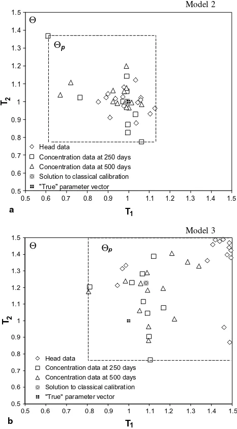
The estimated parameter values^h

ðv;l;tÞand^hfor

mod-els 2 and 3 are shown inFig. 5a and b, respectively. We refer to ^h _{as the ‘‘solution to classical calibration’’ in}

Fig. 5. The dashed rectangle in each of these ﬁgures, which contains all per-datum parameter estimates, de-ﬁnes the posterior space of acceptable parameter values

H_p_{. A model calibrated using the joint data set (criterion}

(3)) provides a closer match to ﬁeld measurements in some regions of the model domain than others. The residual Rat each speciﬁc location and transport time can be measured in the parameter space by measuring the deviation of each ^h

ðv;l;tÞ from^h(Fig. 5a and b). The

location of ^h

ðv;l;tÞ within the parameter space relative to ^

h _{accounts for the information regarding model and}

measurement errors contained in the residual of(3). In the case of small model error and Gaussian measure-ment error, ^h_{will be close to the true parameter vector}

(e.g., Fig. 5a). In such cases, applying the single-objec-tive calibration may be eﬀecsingle-objec-tive and the conﬁdence intervals obtained by an analysis of the residual of (3) (e.g.,[30]) may be correct. However, the true parameter vector and^h _{may not coincide because of a substantial}

non-Gaussian model error (e.g.,Fig. 5b). Then, the devi-ation of each^h

ðv;l;tÞfrom^h(vectorR) is not equal to the

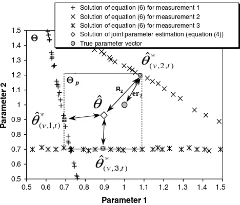
sum of measurement and model error (vectorEr), which is the distance of the per-datum parameter estimates from the true parameter values (Fig. 4), and assigning conﬁdence intervals on model predictions based on the residual of (3) may be unrepresentative of the real situation.

With the residual driven to zero, the per-datum parameter estimates are forced to fully compensate for the error in model structure and measurement error at

0.5

Solution of equation (6) for measurement 1 Solution of equation (6) for measurement 2 Solution of equation (6) for measurement 3 Solution of joint parameter estimation (equation (4)) True parameter vector

θ

ˆ

(9)

each data point (Eqs. (6)). In the presence of model error, the estimated values of the most sensitive para-meters are forced to adjust to the greatest degree during the calibration. The relation between the location inH

of these parameters, expressed as their deviation from the true parameter value in the normalized parameter space, and model error is shown inFig. 6. The influence of model error is measured as the percent difference be-tween the predicted concentration values (using the true parameter values in models 2 and 3), and the error-free observations at each sampling location, derived from the true model. Only those measurement locations that are reached by the plume at 250 days or 500 days are in-cluded in the plot. The effect of model error on ^h

ðv;l;tÞ

is apparent in the observed positive correlation between model error and the distance of each^h

ðv;l;tÞfrom the true

parameter values. In the region where the eﬀect of model error is smaller than 15% (equal to 3 standard deviations of measurement error), which represents the locations where the predicted concentrations are not sensitive to the errors in model structure, the eﬀect of measurement error becomes dominant. These areas of small sensitivity to model error are located near the boundaries of the contaminant plume for model 2 (at 500 days), while for model 3 (at 250 days) the single, low sensitivity site is located close to the center of the plume.

Since the spreading of ^h

ðv;l;tÞ within the parameter

space is dictated by the magnitude of model and mea-surement errors, the size of the posterior parameter spaceH_p_{that contains all per-datum parameter vectors}

will represent the uncertainty due to these errors. In practice, the errors in model structure rather than mea-surement errors are considered more important since they are the main cause of possible failure of a model application[34]. We suggest that the size ofH_p_is

inver-sely proportional to the correctness of the model struc-ture and represents the level of uncertainty in the parameters imposed primarily by the magnitude of model error. For example, the larger H_p _{for model 3}

indicates that model 3 is subject to greater model error that model 2. A comparison of the magnitude of the cal-culated true model error for models 2 and 3 with the size ofH_p_{associated with these models (Fig. 5) demonstrates}

this statement. This relation between the size ofH_p_and

model error may provide a useful tool for evaluating alternative conceptual models (model discrimination). The size of the posterior parameter space H_p _{may also}

oﬀer a reasonable basis for selecting a ‘‘best’’ solution of the minimization problem of classical calibration in

0

Influence of model error

r

Fig. 6. Relation between model error and location of^h

ðv;l;tÞfor model 2 using concentration data at 500 days and model 3 using concentration data at 250 days. Model error is measured as the per cent diﬀerence between model predictions with the true parameter values at each sampling location, and the true concentrations at the same locations and time.

Concentration data at 250 days Concentration data at 500 days Solution to classical calibration "True" parameter vector

p

Concentration data at 250 days Concentration data at 500 days Solution to classical calibration "True" parameter vector

(10)

the case that(3)does not have a unique minimum. Each of these possible solutions can be used in criterion(8)to select the unique per-datum parameter estimates. The resulting volume of the posterior parameter spaces can then be compared to determine the preferred solution of(3).

The rectangular H_p _{shown in} _{Fig. 5} _{is a crude}

approximation of the posterior parameter space. A more informative probabilistic description of H_p _{can be}

ob-tained by a statistical analysis of the locations of ^h ðv;l;tÞ

in H_{. The statistical distributions of the per-datum}

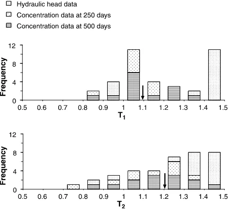
parameter estimates for model 3 are shown in Fig. 7. Since the proposed methodology does not require any assumptions to be made regarding the probabilistic properties of the error, these distributions may be used in testing the validity of the normality assumption and the performance of the joint parameter estimation. The parameter estimates from classical calibration (shown as arrows in Fig. 7) are the (weighted) average of all ^h

ðv;l;tÞ. This ﬁgure demonstrates the inﬂuence of

the weights assigned to diﬀerent data in classical calibra-tion. Assigning higher weights to the hydraulic head data will result in greater values of parameter estimates. The parameter estimates will be smaller if concentration data are weighted more than the hydraulic head data. As suggested earlier in Section3(seeFig. 3),Fig. 7also sug-gests that the problem of non-uniqueness of the single-objective inverse procedures may be a result of error in the model structure. As can be seen in this ﬁgure (see distribution ofT1), certain weights assigned to mea-surements of the dependent variables may result in two local minima in the objective function of the classical

calibration. The location of these local minima in the parameter space will coincide with the two peaks in the distribution of the per-datum parameter estimates forT1. When the model structure is correct (for example the ﬂow solution of model 2), the posterior parameter space is normally distributed around the true parameter values since it is subject only to measurement error (Fig. 8).

The posterior parameter spaceH_p_{may be used in}

sto-chastic modeling to assess the prediction uncertainty associated with model and measurement errors. How-ever, usingH_p_{to evaluate the uncertainty in model}

pre-dictions may result in assigning a level of uncertainty imposed by the maximum model error within the model domain on all sampling locations. Because model error is spatially distributed, location-speciﬁc uncertainty lev-els on the parameters would be more appropriate. We adopt the latter approach. A posterior feasible parame-ter space is estimated for each sampling location based on the range of the per-datum estimates^h

ðv;l;tÞassociated

with this location. For example, the posterior parameter space associated with sampling location 15 is estimated as the region in the parameter space that contains the three per-datum estimates that correspond to the mea-surements of steady-state hydraulic head and concentra-tion at times of 250 and 500 days at this locaconcentra-tion. From these three values, upper and lower bounds are identified for T1 and T2. The location-specific parameter uncer-tainty is then propagated through the model using these values to identify upper and lower bounds on the (loca-tion-specific) model predictions for models 2 and 3. These bounds are shown inFigs. 9 and 10, respectively.

Fig. 7. Statistical distributions of the per-datum estimates of trans-missivity 1 and 2 for model 3. The arrows show the location of the solution of the classical calibration (Eq.(3)).

0.5

0.5 0.6 0.7 0.8 0.9 1 1.1 1.2 1.3 1.4 1.5 0.6

0.7 0.8 0.9 1 1.1 1.2 1.3 1.4 1.5

T1 T2

Steady-state head data True parameter vector

Model 2

(11)

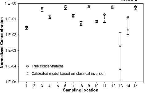
Note that, in this simple example, a uniform probability distribution is assigned to the location-speciﬁc parame-ter uncertainty because of the small number of per-datum parameter estimates associated with each location. The availability of a greater number of location-speciﬁc data will allow a more informative probabilistic descrip-tion of parameter and predicdescrip-tion uncertainty at a given location. Figs. 9 and 10 do not include the sampling locations 2 and 5 because no concentration data were available at these locations as they were not reached by the contaminant within the time frame of 500 days used for model calibration. Although the parameter vec-tor^h _{is used for the estimation of}^h_ðv;l;tÞ_{, it is not taken}

into account in evaluating the posterior parameter space associated with each location. As a result, the predic-tions of the models calibrated using the joint data set (Eq. (3)) are not necessarily included within the esti-mated range of concentration values at 750 days (e.g.,

Fig. 10—locations 1, 8 and 14). These are the locations that contribute the most in the residual of the minimiza-tion problem(3).

Model predictions presented here as a range of equally probable values (Figs. 9 and 10) are based on information on model error for the calibration time frame. In other words, our predictions of probable fu-ture responses of the true system are based on an anal-ysis of model error using past data. However, the ability of the model structure to describe the physical system may deteriorate with time. This behavior may re-sult in prediction bounds that do not bracket the true values (Fig. 9—locations 11 and 14). In sampling loca-tions 11 and 14, the effect of errors in model structure for model 2 on concentrations predicted at 750 days is greater than their effect during the calibration period that was evaluated. Updating the analysis as new data become available may (even partially) resolve this prob-lem. Uninformative (highly uncertain to unacceptable levels) predictions indicate the need for model structure refinement. Refining the model structure will result in a smaller posterior parameter space and lead to a reduc-tion of the predicreduc-tion uncertainty.

6. Summary and conclusions

Errors in model structure (model error) cannot be avoided because they arise from our limited capability to exactly describe the complexity of a physical system. These errors have a significant impact on uncertainty analyses, parameter estimation and model predictions and therefore, they cannot be ignored. A model calibra-tion procedure, complementary to classical inverse methods, that takes model error into account has been presented in this paper. This procedure is based on the concept of a per-datum calibration for capturing the spatial and temporal behavior of model error. A set of per-datum parameter estimates rather than a point esti-mate is obtained by this new method. These parameter estimates define a posterior parameter space that may be translated into a probabilistic description of model predictions. The resulting prediction uncertainty mea-sures the level of confidence in model performance eval-uated in terms of each model prediction. It may represent a more accurate reflection on model predic-tions of the available information, which is required for decision making.

Through a simple example we have shown that per-datum calibration may also provide the means for: (1) evaluating the performance of classical calibration in terms of the predictive capability of the model, (2) test-ing the validity of assumptions regardtest-ing error statistical distributions underlying the estimation of parameters and their conﬁdence intervals in classical single-objec-tive calibration, (3) selecting the best solution of the Model 2

1.E-05 1.E-04 1.E-03 1.E-02 1.E-01 1.E+00

1 2 3 4 5 6 7 8 9 10 11 12 13 14 15 Sampling location

n

oi

t

ar

t

n

e

c

n

o

C

d

e

zil

a

mr

o

N True concentrations

Calibrated model based on classical inversion

Fig. 9. Concentration estimates for model 2 at time 750 days. The error bars show the range of prediction uncertainty associated with accounting for model and measurement errors. Sampling locations are shown inFig. 1.

Model 3

1.E-03 1.E-02 1.E-01 1.E+00

1 2 3 4 5 6 7 8 9 10 11 12 13 14 15 Sampling location

Normaliz

ed Concentration

True concentrations

Calibrated model based on classical inversion

(12)

minimization problem of classical calibration in the case that it does not have a unique solution, and (4) evaluat-ing alternative conceptual models in terms of the cor-rectness of the model structure.

Acknowledgments

Discussions with Roger Beckie were helpful for for-mulating our ideas. This work was supported by a schol-arship to P. Gaganis provided by the State Scholschol-arship Foundation of Greece and a grant from the Natural Sci-ences and Engineering Research Council of Canada.

References

[1] Beck MB. Water quality modeling: a review of the analysis of uncertainty. Water Resour Res 1987;23:1393–442.

[2] Beckie R. Measurement scale, network sampling scale, and

ground water model parameters. Water Resour Res

1996;32(1):65–76.

[3] Beven KJ, Binley AM. The future of distributed models: model calibration and uncertainty prediction. Hydrol Process 1992;6:279–98.

[4] Bredehoeft J. The conceptualization model problem—surprise. Hydrogeol J 2005;13:37–46.

[5] Carrera J, Alcolea A, Medina A, Hidalgo J, Slooten LJ. Inverse problem in hydrogeology. Hydrogeol J 2005;13:206–22. [6] Carrera J, Neuman SP. Estimation of aquifer parameters under

transient and steady state conditions: 1. Maximum likelihood method incorporating prior information. Water Resour Res 1986;22:199–210.

[7] Carrera J, Neuman SP. Estimation of aquifer parameters under transient and steady state conditions: 2. Uniqueness, stability, and solution algorithms. Water Resour Res 1986;22:211–27. [8] Christensen S, Cooley RL. Evaluation of prediction intervals for

expressing uncertainties in groundwater ﬂow model predictions. Water Resour Res 1999;35:2627–39.

[9] Cooley RL. Incorporation of prior information on parameters into nonlinear regression groundwater models. 1. Theory. Water Resour Res 1982;18:965–76.

[10] Cooley RL. Incorporation of prior information on parameters into nonlinear regression groundwater models. 2. Applications. Water Resour Res 1983;19:662–76.

[11] Cooley RL, Konikow LF, Naﬀ RL. Nonlinear-regression ground-water ﬂow modeling of a deep regional aquifer system. Water Resour Res 1986;22:1759–78.

[12] Dagan G. Flow and transport in porous formations. New York: Springer-Verlag; 1989.

[13] Dagan G, Neuman SP, editorsSubsurface ﬂow and transport: a stochastic approach. United Kingdom: Cambridge University Press; 1997.

[14] Feder J. Fractals. New York: Plenum Press; 1988.

[15] Freeze RA, Massmann J, Smith L, Sperling T, James B. Hydrological decision analysis: 1. A framework. Ground Water 1990;28:738–66.

[16] Gaganis P, Smith L. A Bayesian approach to the quantiﬁcation of the eﬀect of model error on the predictions of groundwater models. Water Resour Res 2001;37:2309–22.

[17] Gelhar LW. Stochastic subsurface hydrogeology. Englewood Cliﬀs, NJ: Prentice-Hall; 1993.

[18] Gupta HV, Sorooshian S, Yapo PO. Toward improved calibra-tion of hydrologic models: multiple and noncommensurable measures of information. Water Resour Res 1998;34:751–63. [19] Hill CM. A review of experimental design procedures for

regression and model discrimination. Technometrics 1978;20: 15–21.

[20] Hill CM. Methods and guidelines for eﬀective model calibration. US Geological Survey Water-Resources Investigations Report 98-4005, 1998.

[21] James AL, Oldenburg CM. Linear and Monte Carlo uncertainty analysis for subsurface contaminant transport simulation. Water Resour Res 1997;33:2495–508.

[22] Kitanidis PK, Vomvoris EG. A geostatistical approach to the inverse problem in groundwater modeling (steady state) and one-dimensional simulations. Water Resour Res 1983;19:677–90. [23] Konikow LF, Bredehoeft JD. Ground-water models cannot be

validated. Adv Water Resour 1992;15:75–83.

[24] Luis SJ, McLaughlin D. A stochastic approach to model validation. Adv Water Resour 1992;15:15–32.

[25] Mckay MD, Beckman RJ, Conover WJ. A comparison of three methods for selecting values of input variables in the analysis of output from a computer code. Technometrics 1979;2:239–45. [26] McLaughlin D, Townley LR. A reassessment of the groundwater

inverse problem. Water Resour Res 1996;32:1131–61.

[27] Morgan MG, Henrion M, Small M. Uncertainty: a guide to dealing with uncertainty in quantitative risk and policy analy-sis. United Kingdom: Cambridge University Press; 1990. [28] Neuman SP. Calibration of distributed groundwater ﬂow models

viewed as a multiple-objective decision process under uncertainty. Water Resour Res 1973;9:1006–21.

[29] Neuman SP. Maximum likelihood Bayesian averaging of uncer-tain model predictions. Stoch Env Res Risk A 2003;17:291–305. [30] Poeter EP, Hill MC. Inverse models: a necessary next step in

ground-water modeling. Ground Water 1997;35:250–60. [31] Poeter EP, Hill MC. Documentation of UCODE, a computer

code for universal inverse modelling. USGS Water-resources investigation report 98-4080, 1998.

[32] Schwarz G. Estimating the dimension of a model. Ann Statist 1978;6:461–5.

[33] Smith L, Gaganis P. Strontium-90 migration to water wells at the chernobyl nuclear power plant: re-evaluation of a decision model. Environ Eng Geosci 1998;IV:161–74.

[34] Sun N-Z, Yang S-L, Yeh WW-G. A proposed stepwise regression method for model structure identiﬁcation. Water Resour Res 1998;34:2561–72.

[35] Sun N, Yeh WW-G. Identiﬁcation of parameter structure in groundwater inverse problems. Water Resour Res 1985;21: 869–83.

[36] Weiss W, Smith L. Eﬃcient and responsible use of prior information in inverse methods. Ground Water 1998;36:151–63. [37] Weiss W, Smith L. Parameter space methods in joint parameter

estimation for groundwater models. Water Resour Res

1998;24:647–61.

[38] Yapo PO, Gupta HV, Sorooshian S. Multi-objective global optimization for hydrologic models. J Hydrol 1998;204:83–97. [39] Ye M, Neuman SP, Meyer PD. Maximum likelihood Bayesian

averaging of spatial variability models in unsaturated fractured tuﬀ. Water Resour Res 2004;40:W05113.

[40] Zhang D. Stochastic methods for ﬂow in porous media. San Diego: Academic Press; 2001.