Numerical Analysis Using MATLAB and Excel Steven T. Karris

Orchard Publications www.orchardpublications.com

Numerical

Analysis

Using MATLAB® and Excel®

ISBN-13: 978-11-9934404-004-11

Orchard Publications Visit us on the Internet www.orchardpublications.com or email us: info@orchardpublications.com

Steven T. Karris is the president and founder of Orchard Publications, has undergraduate and graduate degrees in electrical engineering, and is a registered professional engineer in

California and Florida. He has more than 35 years of professional engineering experience and more than 30 years of teaching experience as an adjunct professor, most recently at UC Berkeley, California.

This text includes the following chapters and appendices:

• Introduction to MATLAB • Root Approximations • Sinusoids and Complex Numbers • Matrices and Determinants • Review of Differential Equations • Fourier, Taylor, and Maclaurin Series • Finite Differences and Interpolation • Linear and Parabolic Regression • Solution of Differential Equations by Numerical Methods • Integration by Numerical Methods • Difference Equations • Partial Fraction Expansion • The Gamma and Beta Functions • Orthogonal Functions and Matrix Factorizations • Bessel, Legendre, and Chebyshev Polynomials • Optimization Methods • Difference Equations in Discrete-Time Systems • Introduction to Simulink • Ill-Conditioned Matrices

Each chapter contains numerous practical applications supplemented with detailed instructions for using MATLAB and/or Excel to obtain quick solutions.

Students and working professionals will find NNuummeerriiccaall AAnnaallyyssiiss UUssiinngg MMAATTLLAABB®® a

anndd EExxcceell®®,, TThhiirrdd EEddiittiioonn, to be a concise and easy-to-learn text. It provides com-plete, clear, and detailed explanations of the principal numerical analysis methods and well known functions used in science and engineering. These are illustrated with many real-world examples.

Numerical Analysis

Using MATLAB® and Excel®

Third Edition

Numerical Analysis

Using MATLAB

®

and Excel

®

Third Edition

Steven T. Karris

Numerical Analysis Using MATLAB® and Excel®, Third Edition

Copyright ” 2007 Orchard Publications. All rights reserved. Printed in the United States of America. No part of this publication may be reproduced or distributed in any form or by any means, or stored in a data base or retrieval system, without the prior written permission of the publisher.

Direct all inquiries to Orchard Publications, info@orchardpublications.com

Product and corporate names are trademarks or registered trademarks of the Microsoft™ Corporation and The MathWorks™, Inc. They are used only for identification and explanation, without intent to infringe.

Library of Congress Cataloging-in-Publication Data

Library of Congress Control Number: 2007922100

Copyright TX 5-589-152

ISBN-13: 978-1-934404-04-1

ISBN-10: 1-934404-04-7

Disclaimer

Preface

Numerical analysis is the branch of mathematics that is used to find approximations to difficult problems such as finding the roots of non−linear equations, integration involving complex expressions and solving differential equations for which analytical solutions do not exist. It is applied to a wide variety of disciplines such as business, all fields of engineering, computer science, education, geology, meteorology, and others.

Years ago, high−speed computers did not exist, and if they did, the largest corporations could only afford them; consequently, the manual computation required lots of time and hard work. But now that computers have become indispensable for research work in science, engineering and other fields, numerical analysis has become a much easier and more pleasant task.

This book is written primarily for students/readers who have a good background of high−school algebra, geometry, trigonometry, and the fundamentals of differential and integral calculus.* A prior knowledge of differential equations is desirable but not necessary; this topic is reviewed in Chapter 5.

One can use Fortran, Pascal, C, or Visual Basic or even a spreadsheet to solve a difficult problem. It is the opinion of this author that the best applications programs for solving engineering problems are 1) MATLAB which is capable of performing advanced mathematical and engineering computations, and 2) the Microsoft Excel spreadsheet since the versatility offered by spreadsheets have revolutionized the personal computer industry. We will assume that the reader has no prior knowledge of MATLAB and limited familiarity with Excel.

We intend to teach the student/reader how to use MATLAB via practical examples and for detailed explanations he/she will be referred to an Excel reference book or the MATLAB User’s Guide. The MATLAB commands, functions, and statements used in this text can be executed with either MATLAB Student Version 12 or later. Our discussions are based on a PC with Windows XP platforms but if you have another platform such as Macintosh, please refer to the appropriate sections of the MATLAB’s User Guide that also contains instructions for installation.

MATLAB is an acronym for MATrix LABoratory and it is a very large computer application which is divided to several special application fields referred to as toolboxes. In this book we will be using the toolboxes furnished with the Student Edition of MATLAB. As of this writing, the latest release is MATLAB Student Version Release 14 and includes SIMULINK which is a

software package used for modeling, simulating, and analyzing dynamic systems. SIMULINK is not discussed in this text; the interested reader may refer to Introduction to Simulink with Engineering Applications, ISBN 0−9744239−7−1. Additional information including purchasing the software may be obtained from The MathWorks, Inc., 3 Apple Hill Drive, Natick, MA 01760−2098. Phone: 508 647−7000, Fax: 508 647−7001, e−mail: info@mathwork.com and web site http://www.mathworks.com.

The author makes no claim to originality of content or of treatment, but has taken care to present definitions, statements of physical laws, theorems, and problems.

Chapter 1 is an introduction to MATLAB. The discussion is based on MATLAB Student Version 5 and it is also applicable to Version 6. Chapter 2 discusses root approximations by numerical methods. Chapter 3 is a review of sinusoids and complex numbers. Chapter 4 is an introduction to matrices and methods of solving simultaneous algebraic equations using Excel and MATLAB. Chapter 5 is an abbreviated, yet practical introduction to differential equations, state variables, state equations, eigenvalues and eigenvectors. Chapter 6 discusses the Taylor and Maclaurin series. Chapter 7 begins with finite differences and interpolation methods. It concludes with applications using MATLAB. Chapter 8 is an introduction to linear and parabolic regression. Chapters 9 and 10 discuss numerical methods for differentiation and integration respectively. Chapter 11 is a brief introduction to difference equations with a few practical applications. Chapters 12 is devoted to partial fraction expansion. Chapters 13, 14, and 15 discuss certain interesting functions that find wide application in science, engineering, and probability. This text concludes with Chapter 16 which discusses three popular optimization methods.

New to the Third Edition

This is an extensive revision of the first edition. The most notable changes are the inclusion of Fourier series, orthogonal functions and factorization methods, and the solutions to all end−of−

chapter exercises. It is in response to many readers who expressed a desire to obtain the solutions in order to check their solutions to those of the author and thereby enhancing their knowledge. Another reason is that this text is written also for self−study by practicing engineers who need a review before taking more advanced courses such as digital image processing. The author has prepared more exercises and they are available with their solutions to those instructors who adopt this text for their class.

Another change is the addition of a rather comprehensive summary at the end of each chapter. Hopefully, this will be a valuable aid to instructors for preparation of view foils for presenting the material to their class.

The last major change is the improvement of the plots generated by the latest revisions of the MATLAB® Student Version, Release 14.

Orchard Publications Fremont, California

Table of Contents

1

Introduction to MATLAB 1−1

1.1 Command Window...1−1 1.2 Roots of Polynomials...1−3 1.3 Polynomial Construction from Known Roots ...1−4 1.4 Evaluation of a Polynomial at Specified Values ...1−5 1.5 Rational Polynomials ...1−8 1.6 Using MATLAB to Make Plots...1−9 1.7 Subplots...1−18 1.8 Multiplication, Division and Exponentiation...1−19 1.9 Script and Function Files...1−26 1.10 Display Formats ...1−31 1.11 Summary ...1−33 1.12 Exercises...1−37 1.13 Solutions to End−of−Chapter Exercises ...1−38

MATLAB Computations: Entire chapter

2

Root Approximations 2−1

2.1 Newton’s Method for Root Approximation...2−1 2.2 Approximations with Spreadsheets...2−7 2.3 The Bisection Method for Root Approximation ...2−19 2.4 Summary...2−27 2.5 Exercises ...2−28 2.6 Solutions to End−of−Chapter Exercises ...2−29

MATLAB Computations: Pages 2−2 through 2−7, 2−14, 2−21 through 2−23, 2−29 through 2−34

Excel Computations: Pages 2−8 through 2−19, 2−24 through 2−26

3

Sinusoids and Phasors 3−1

3.8 Exponential and Polar Forms of Phasors ...3−13 3.9 Summary ...3−24 3.10 Exercises...3−27 3.11 Solutions to End−of−Chapter Exercises...3−28

MATLAB Computations: Pages 3−15 through 3−23, 3−28 through 3−31 Simulink Modeling: Pages 3−16 through 3−23

4

Matrices and Determinants 4−1

4.1 Matrix Definition...4−1 4.2 Matrix Operations ...4−2 4.3 Special Forms of Matrices...4−5 4.4 Determinants ...4−9 4.5 Minors and Cofactors ...4−13 4.6 Cramer’s Rule ...4−18 4.7 Gaussian Elimination Method...4−20 4.8 The Adjoint of a Matrix ...4−22 4.9 Singular and Non−Singular Matrices ...4−22 4.10 The Inverse of a Matrix...4−23 4.11 Solution of Simultaneous Equations with Matrices ...4−25 4.12 Summary ...4−32 4.13 Exercises ...4−36 4.14 Solutions to End−of−Chapter Exercises ...4−38

MATLAB Computations: Pages 4−3, 4−5 through 4−8, 4−10, 4−12, 4−3, 4−5, 4−19 through 4−20, 4−24, 4−26, 4−28, 4−30, 4−38, 4−41, 4−43 Excel Computations: Pages 4−28 through 4−29, 4−42 through 4−43

5.13 Exercises ... 5−47 5.14 Solutions to End−of−Chapter Exercises... 5−49

MATLAB Computations: Pages 5−11, 5−13 through 5−14, 5−16 through 5−17, 5−19, 5−23, 5−33 through 5−35, 5−37,

5−49 through 5−53, 5−55

6

Fourier, Taylor, and Maclaurin Series 6−1

6.1 Wave Analysis ...6−1 6.2 Evaluation of the Coefficients ...6−2 6.3 Symmetry ...6−7 6.4 Waveforms in Trigonometric Form of Fourier Series ...6−12 6.5 Alternate Forms of the Trigonometric Fourier Series ...6−25 6.6 The Exponential Form of the Fourier Series ...6−29 6.7 Line Spectra ...6−33 6.8 Numerical Evaluation of Fourier Coefficients ...6−36 6.9 Power Series Expansion of Functions ...6−40 6.10 Taylor and Maclaurin Series ...6−41 6.11 Summary ...6−48 6.12 Exercises ...6−51 6.13 Solutions to End−of−Chapter Exercises ...6−53

MATLAB Computations: Pages 6−35, 6−45, 6−58 through 6−61 Excel Computations: Pages 6−37 through 6−39

7

Finite Differences and Interpolation 7−1

7.1 Divided Differences ... 7−1 7.2 Factorial Polynomials ... 7−6 7.3 Antidifferences ... 7−12 7.4 Newton’s Divided Difference Interpolation Method ... 7−15 7.5 Lagrange’s Interpolation Method ... 7−17 7.6 Gregory−Newton Forward Interpolation Method ... 7−19 7.7 Gregory−Newton Backward Interpolation Method ... 7−21 7.8 Interpolation with MATLAB ... 7−24 7.9 Summary ... 7−39 7.10 Exercises ... 7−44 7.11 Solutions to End−of−Chapter Exercises ... 7−45

MATLAB Computations: Pages 7−8 through 7−9, 7−13 through 7−15, 7−26 through 7−38, 7−45 through 7−46, 7−48, 7−50, 7−52

8

Linear and Parabolic Regression 8−1

8.1 Curve Fitting ...8−1 8.2 Linear Regression ...8−2 8.3 Parabolic Regression ...8−7 8.4 Regression with Power Series Approximations ...8−14 8.5 Summary ...8−24 8.6 Exercises ...8−26 8.7 Solutions to End−of−Chapter Exercises ...8−28

MATLAB Computations: Pages 8−11 through 8−14, 8−17 through 8−23, 8−30 through 8−34

Excel Computations: Pages 8−5 through 8−10, 8−15 through 8−19, 8−28 through 8−32

9

Solution of Differential Equations by Numerical Methods 9−1

9.1 Taylor Series Method ... 9−1 9.2 Runge−Kutta Method ... 9−5 9.3 Adams’ Method ... 9−13 9.4 Milne’s Method ... 9−15 9.5 Summary ... 9−17 9.6 Exercises ... 9−20 9.7 Solutions to End−of−Chapter Exercises ... 9−21

MATLAB Computations: Pages 9−5, 9−9 through 9−12, 9−21 through 9−23 Excel Computations: Page 9−2, 9−14, 9−22 through 9−26

10

Integration by Numerical Methods 10−1

10.1 The Trapezoidal Rule ... 10−1 10.2 Simpson’s Rule ... 10−6 10.3 Summary ... 10−14 10.4 Exercises ... 10−15 10.5 Solution to End−of−Chapter Exercises ... 10−16

MATLAB Computations: Pages 10−3 through 10−6, 10−9 through 10−13, 10−16, 10−18 through 10−21

Excel Computations: Pages 10−10, 10−19 through 10−21

11

Difference Equations 11−1

11.4 Summary ...11−11 11.5 Exercises ... 11−13 11.6 Solutions to End−of−Chapter Exercises ...11−14

12

Partial Fraction Expansion 12−1

12.1 Partial Fraction Expansion ...12−1 12.2 Alternate Method of Partial Fraction Expansion ...12−13 12.3 Summary ...12−19 12.4 Exercises ...12−22 12.5 Solutions to End−of−Chapter Exercises ...12−23

MATLAB Computations: Pages 12−3 through 12−5, 12−9 through 12−12, 12−16 through 12-18, 12−23 through 12−28

13

The Gamma and Beta Functions and Distributions 13−1 13.1 The Gamma Function ...13−1 13.2 The Gamma Distribution ...13−16 13.3 The Beta Function ...13−17 13.4 The Beta Distribution ...13−20 13.5 Summary ...13−22 13.6 Exercises ...13−24 13.7 Solutions to End−of−Chapter Exercises ...13−25

MATLAB Computations: Pages 13−3, 13−5, 13−10, 13−19, 13−25

Excel Computations: Pages 13−5, 13−10, 13−16 through 13−17, 13−19, 13−21

14

Orthogonal Functions and Matrix Factorizations 14−1 14.1 Orthogonal Functions ...14−1 14.2 Orthogonal Trajectories ...14−2 14.3 Orthogonal Vectors ...14−4 14.4 The Gram−Schmidt Orthogonalization Procedure ...14−7 14.5 The LU Factorization ...14−9 14.6 The Cholesky Factorization ...14−23 14.7 The QR Factorization ...14−25 14.8 Singular Value Decomposition ...14−28 14.9 Summary ...14−30 14.10 Exercises ...14−32 14.11 Solutions to End−of−Chapter Exercises ...14−34

15

Bessel, Legendre, and Chebyshev Functions 15−1

15.1 The Bessel Function ...15−1 15.2 Legendre Functions ...15−10 15.3 Laguerre Polynomials ...15−21 15.4 Chebyshev Polynomials ...15−22 15.5 Summary ...15−27 15.6 Exercises ...15−32 15.7 Solutions to End−of−Chapter Exercises ...15−33

MATLAB Computations: Pages 15−3 through 15−4, 15−6, 15−9,

14−19 through 15−22, 15−25, 15−33, 15−35 through 15−37 Excel Computations: Pages 15−5, 15−9

16

Optimization Methods 16−1

16.1 Linear Programming ... 16−1 16.2 Dynamic Programming ...16−4 16.3 Network Analysis ...16−14 16.4 Summary ...16−19 16.5 Exercises ...15−20 16.6 Solutions to End−of−Chapter Exercises ...15−22

MATLAB Computations: Pages 16−3

Excel Computations: Pages 16−4, 16−23, 16−25 through 16−27

A

Difference Equations in Discrete−Time Systems A−1 A.1 Recursive Method for Solving Difference Equations... A−1 A.2 Method of Undetermined Coefficients ...A−1

MATLAB Computations: Pages A−4, A−7, A−9

B

Introduction to Simulink® B−1

B.1 Simulink and its Relation to MATLAB ... B−1 B.2 Simulink Demos ...B−20

MATLAB Computations and Simulink Modeling: Entire Appendix B

C

Ill-Conditioned Matrices C−1

MATLAB Computations: Pages C−1, C−4 through C−5

References R−1

Chapter 1

Introduction to MATLAB

his chapter is an introduction of the basic MATLAB commands and functions, procedures for naming and saving the user generated files, comment lines, access to MATLAB’s Editor/ Debugger, finding the roots of a polynomial, and making plots. Several examples are pro-vided with detailed explanations. Throughout this text, a left justified horizontal bar will denote the beginning of an example, and a right justified horizontal bar will denote the end of the exam-ple. These bars will not be shown whenever an example begins at the top of a page or at the bot-tom of a page. Also, when one example follows immediately after a previous example, the right justified bar will be omitted.

1.1 Command Window

To distinguish the screen displays from the user commands, important terms and MATLAB func-tions, we will use the following conventions:

Click: Click the left button of the mouse

Courier Font: Screen displays

Helvetica Font: User inputs at MATLAB’s command window prompt EDU>>*

Helvetica Bold: MATLAB functions

Bold Italic: Important terms and facts, notes, and file names

When we first start MATLAB, we see the toolbar on top of the command screen and the prompt EDU>>. This prompt is displayed also after execution of a command; MATLAB now waits for a new command from the user. We can use the Editor/Debugger to write our program, save it, and return to the command screen to execute the program as explained below.

To use the Editor/Debugger:

1. From the File menu on the toolbar, we choose New and click on M−File. This takes us to the Editor Window where we can type our script (list of statements) for a new file, or open a previ-ously saved file. We must save our program with a file name which starts with a letter. Impor-tant! MATLAB is case sensitive, that is, it distinguishes between upper− and lower−case let-ters. Thus, t and T are two different characters in MATLAB language. The files that we create are saved with the file name we use and the extension .m; for example, myfile01.m. It is a good

* EDU>> is the MATLAB prompt in the Student Version.

T

Chapter 1 Introduction to MATLAB

practice to save the script in a file name that is descriptive of our script content. For instance, if the script performs some matrix operations, we ought to name and save that file as matrices01.m or any other similar name. We should also use a separate disk to backup our files.

2. Once the script is written and saved as an m−file, we may exit the Editor/Debugger window by clicking on Exit Editor/Debugger of the File menu, and MATLAB returns to the command window.

3. To execute a program, we type the file name without the .m extension at the EDU>> prompt; then, we press <enter> and observe the execution and the values obtained from it. If we have saved our file in drive a or any other drive, we must make sure that it is added it to the desired directory in MATLAB’s search path. The MATLAB User’s Guide provides more information on this topic.

Henceforth, it will be understood that each input command is typed after the EDU>> prompt and followed by the <enter> key.

The command help matlab iofun will display input/output information. To get help with other MATLAB topics, we can type help followed by any topic from the displayed menu. For example, to get information on graphics, we type helpmatlab graphics. We can also get help from the Help pull− down menu. The MATLAB User’s Guide contains numerous help topics.

To appreciate MATLAB’s capabilities, we type demo and we see the MATLAB Demos menu. We can do this periodically to become familiar with them. Whenever we want to return to the com-mand window, we click on the Close button.

When we are done and want to leave MATLAB, we type quit or exit. But if we want to clear all previous values, variables, and equations without exiting, we should use the clear command. This command erases everything; it is like exiting MATLAB and starting it again. The clc command clears the screen but MATLAB still remembers all values, variables and equations which we have already used. In other words, if we want MATLAB to retain all previously entered commands, but leave only the EDU>> prompt on the upper left of the screen, we can use the clc command.

All text after the % (percent) symbol is interpreted by MATLAB as a comment line and thus it is ignored during the execution of a program. A comment can be typed on the same line as the func-tion or command or as a separate line. For instance, the statements

conv(p,q) % performs multiplication of polynomials p and q

% The next statement performs partial fraction expansion of p(x) / q(x)

are both correct.

One of the most powerful features of MATLAB is the ability to do computations involving com-plex numbers. We can use either , or to denote the imaginary part of a complex number, such as

or . For example, the statement

z=3−4j

i j

Roots of Polynomials

displays

z =

3.0000 - 4.0000i

In the example above, a multiplication (*) sign between and was not necessary because the complex number consists of numerical constants. However, if the imaginary part is a function or variable such as , we must use the multiplication sign, that is, we must type cos(x)*j or

j*cos(x).

1.2 Roots of Polynomials

In MATLAB, a polynomial is expressed as a row vector of the form . The elements of this vector are the coefficients of the polynomial in descending order. We must include terms whose coefficients are zero.

We can find the roots of any polynomial with the roots(p) function where p is a row vector con-taining the polynomial coefficients in descending order.

Example 1.1

Find the roots of the polynomial

(1.1) Solution:

The roots are found with the following two statements. We have denoted the polynomial as p1, and the roots as roots_ p1.

p1=[1 −10 35 −50 24] % Specify the coefficients of p1(x)

p1 =

1 -10 35 -50 24

roots_ p1=roots(p1) % Find the roots of p1(x)

roots_p1 = 4.0000 3.0000 2.0000 1.0000

We observe that MATLAB displays the polynomial coefficients as a row vector, and the roots as a column vector.

4 j

x ( ) cos

a_n a_{n 1}– a2 a1 a0

[ ]

a_i

Chapter 1 Introduction to MATLAB

Example 1.2

Find the roots of the polynomial

(1.2) Solution:

There is no cube term; therefore, we must enter zero as its coefficient. The roots are found with the statements below where we have defined the polynomial as p2, and the roots of this polynomial as

roots_ p2.

p2=[1 −7 0 16 25 52]

p2 =

1 -7 0 16 25 52

roots_ p2=roots(p2)

roots_ p2 =

6.5014 2.7428 -1.5711 -0.3366 + 1.3202i -0.3366 - 1.3202i

The result indicates that this polynomial has three real roots, and two complex roots. Of course, complex roots always occur in complex conjugate* pairs.

1.3 Polynomial Construction from Known Roots

We can compute the coefficients of a polynomial from a given set of roots with the poly(r) func-tion where r is a row vector containing the roots.

Example 1.3

It is known that the roots of a polynomial are . Compute the coefficients of this polynomial.

Solution:

We first define a row vector, say , with the given roots as elements of this vector; then, we find the coefficients with the poly(r) function as shown below.

* By definition, the conjugate of a complex number is

p₂( )x = x5–7x4+16x2+25x+52

A = a+jb A∗ = a jb– 1 2 3 and 4, , ,

Evaluation of a Polynomial at Specified Values

r3=[1 2 3 4] % Specify the roots of the polynomial

r3 =

1 2 3 4

poly_r3=poly(r3) % Find the polynomial coefficients

poly_r3 =

1 -10 35 -50 24

We observe that these are the coefficients of the polynomial of Example 1.1.

Example 1.4

It is known that the roots of a polynomial are . Find the coeffi-cients of this polynomial.

Solution:

We form a row vector, say , with the given roots, and we find the polynomial coefficients with the poly(r) function as shown below.

r4=[ −1 −2 −3 4+5j 4−5j ]

r4 =

Columns 1 through 4

-1.0000 -2.0000 -3.0000 -4.0000 + 5.0000i Column 5

-4.0000 - 5.0000i

poly_r4=poly(r4)

poly_r4 =

1 14 100 340 499 246

Therefore, the polynomial is

(1.3)

1.4 Evaluation of a Polynomial at Specified Values

The polyval(p,x) function evaluates a polynomial at some specified value of the indepen-dent variable .

p₁( )x

1 2 3 4, – , – , +j5 and 4, –j5 –

r4

p₄( )x = x5+14x4+100x3+340x2+499x+246

Chapter 1 Introduction to MATLAB

Example 1.5

Evaluate the polynomial

(1.4)

at .

Solution:

p5=[1 −3 0 5 −4 3 2]; % These are the coefficients

% The semicolon (;) after the right bracket suppresses the display of the row vector % that contains the coefficients of p5.

%

val_minus3=polyval(p5, −3)% Evaluate p5 at x=−3. No semicolon is used here % because we want the answer to be displayed

val_minus3 = 1280

Other MATLAB functions used with polynomials are the following:

conv(a,b) − multiplies two polynomials a and b

[q,r]=deconv(c,d) −divides polynomial c by polynomial d and displays the quotient q and remain-der r.

polyder(p) − produces the coefficients of the derivative of a polynomial p.

Example 1.6

Let

(1.5)

Compute the product with the conv(a,b) function.

Solution:

p1=[1 −3 0 5 7 9]; p2=[2 0 −8 0 4 10 12]; p1p2=conv(p1,p2)

p1p2 =

2 -6 -8 34 18 -24 -74 -88 78 166 174 108

Therefore,

p₅( )x = x6–3x5+5x3–4x2+3x+2 x = –3

p₁ = x5–3x4+5x2+7x+9

p₂ = 2x6–8x4+4x2+10x+12

Evaluation of a Polynomial at Specified Values

We can write MATLAB statements in one line if we separate them by commas or semicolons. Commas will display the results whereas semicolons will suppress the display.

Example 1.7

Let

(1.6)

Compute the quotient using the deconv(p,q) function.

Solution:

p3=[1 0 −3 0 5 7 9]; p4=[2 −8 0 0 4 10 12]; [q,r]=deconv(p3,p4)

q =

0.5000 r =

0 4 -3 0 3 2 3

Therefore, the quotient and remainder are

Example 1.8

Let

(1.7)

Compute the derivative using the polyder(p) function.

Solution:

p5=[2 0 −8 0 4 10 12]; der_p5=polyder(p5)

der_p5 =

12 0 -32 0 8 10

Therefore,

p₁Þp₂ = 2x11–6x10–8x9+34x8+18x7–24x6

74x5–88x4+78x3+166x2+174x+108

–

p3 x 7

3x5

– +5x3+7x+9 =

p4 2x 6

8x5

– +4x2+10x+12 =

p3⁄p4

q x( ) r x( )

q x( ) = 0.5 r x( ) = 4x5–3x4+3x2+2x+3

p5 2x 6

8x4

– +4x2+10x+12 =

Chapter 1 Introduction to MATLAB

1.5 Rational Polynomials

Rational Polynomials are those which can be expressed in ratio form, that is, as

(1.8)

where some of the terms in the numerator and/or denominator may be zero. We can find the roots of the numerator and denominator with the roots(p) function as before.

Example 1.9

Let

(1.9)

Express the numerator and denominator in factored form, using the roots(p) function.

Solution:

num=[1 −3 0 5 7 9]; den=[2 0 −8 0 4 10 12];% Do not display num and den coefficients roots_num=roots(num), roots_den=roots(den) % Display num and den roots

roots_num =

2.4186 + 1.0712i 2.4186 - 1.0712i -1.1633 -0.3370 + 0.9961i -0.3370 - 0.9961i

roots_den =

1.6760 + 0.4922i 1.6760 - 0.4922i -1.9304 -0.2108 + 0.9870i -0.2108 - 0.9870i -1.0000

As expected, the complex roots occur in complex conjugate pairs.

For the numerator, we have the factored form

and for the denominator, we have

dp5⁄dx 12x 5

32x3

– +4x2+8x+10 =

R x( ) Num x( ) Den x( )

--- bnx

n

b_{n 1}– x

n 1–

b_{n 2}– x

n 2– _…

b1x b0

+ + + + +

a_mxm a_{m 1}– x

m 1–

a_{m 2}– x

m 2– _…

a1x a0

+ + + + +

---= =

R x( ) pnum p_den

--- x

5

3x4

– +5x2+7x+9 2x6–8x4+4x2+10x+12

---= =

p_num = (x 2.4186– –j1.0712)⋅(x 2.4186– +j1.0712)⋅(x+1.1633)⋅

x+0.3370 j0.9961–

( )⋅(x+0.3370+j0.9961)

pden = (x 1.6760– –j0.4922)⋅(x 1.6760– +j0.4922)⋅(x+1.9304)⋅

x+0.2108 j– 0.9870

Using MATLAB to Make Plots

We can also express the numerator and denominator of this rational function as a combination of linear and quadratic factors. We recall that in a quadratic equation of the form

whose roots are and , the negative sum of the roots is equal to the coef-ficient of the term, that is, , while the product of the roots is equal to the constant term , that is, . Accordingly, we form the coefficient by addition of the complex conjugate roots and this is done by inspection; then we multiply the complex conjugate roots to obtain the constant term using MATLAB as indicated below.

(2.4186+1.0712i)*(2.4186 −1.0712i) % Form the product of the 1st set of complex conjugates

ans = 6.9971

(−0.3370+0.9961i)*(−0.3370−0.9961i) % Form the product of the 2nd set of complex conjugates

ans = 1.1058

(1.6760+0.4922i)*(1.6760−0.4922i)

ans = 3.0512

(−0.2108+0.9870i)*(−0.2108−0.9870i)

ans = 1.0186

1.6 Using MATLAB to Make Plots

Quite often, we want to plot a set of ordered pairs. This is a very easy task with the MATLAB plot(x,y) command which plots versus . Here, is the horizontal axis (abscissa) and is the vertical axis (ordinate).

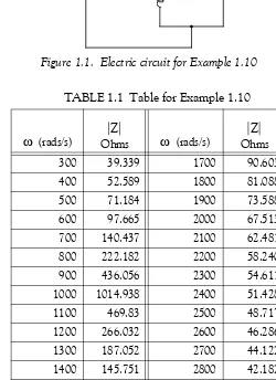
Example 1.10

Consider the electric circuit of Figure 1.1, where the radian frequency (radians/second) of the applied voltage was varied from to in steps of radians/second, while the amplitude was held constant. The ammeter readings were then recorded for each frequency. The magnitude of the impedance was computed as and the data were tabulated in Table 1.1.

Plot the magnitude of the impedance, that is, versus radian frequency .

Solution:

We cannot type (omega) in the MATLAB command window, so we will use the English letter w instead.

x2_{+bx+c = 0 x}

1 x2

b x –(x₁+x₂) = b

c x₁⋅x₂ = c b

c

y x x y

ω

300 3000 100

Z Z = V A⁄

Z ω

Chapter 1 Introduction to MATLAB

Figure 1.1. Electric circuit for Example 1.10

If a statement, or a row vector is too long to fit in one line, it can be continued to the next line by typing three or more periods, then pressing <enter> to start a new line, and continue to enter data. This is illustrated below for the data of w and z. Also, as mentioned before, we use the semi-colon (;) to suppress the display of numbers which we do not care to see on the screen.

The data are entered as follows:

w=[300 400 500 600 700 800 900 1000 1100 1200 1300 1400.... % Use 4 periods to continue 1500 1600 1700 1800 1900 2000 2100 2200 2300 2400 2500....

TABLE 1.1 Table for Example 1.10

(rads/s) _Ohms (rads/s) _Ohms

300 39.339 1700 90.603

400 52.589 1800 81.088

500 71.184 1900 73.588

600 97.665 2000 67.513

700 140.437 2100 62.481

800 222.182 2200 58.240

900 436.056 2300 54.611

1000 1014.938 2400 51.428

1100 469.83 2500 48.717

1200 266.032 2600 46.286

1300 187.052 2700 44.122

1400 145.751 2800 42.182

1500 120.353 2900 40.432

1600 103.111 3000 38.845

A

V _L

C R2

R1

Using MATLAB to Make Plots

2600 2700 2800 2900 3000]; % Use semicolon to suppress display of these numbers %

z=[39.339 52.789 71.104 97.665 140.437 222.182 436.056.... 1014.938 469.830 266.032 187.052 145.751 120.353 103.111.... 90.603 81.088 73.588 67.513 62.481 58.240 54.611 51.468.... 48.717 46.286 44.122 42.182 40.432 38.845];

Of course, if we want to see the values of w or z or both, we simply type w or z, and we press <enter>.

To plot z ( ) versus w ( ), we use the plot(x,y)command. For this example, we use plot(w,z). When this command is executed, MATLAB displays the plot on MATLAB’s graph screen. This plot is shown in Figure 1.2.

Figure 1.2. Plot of impedance versus frequency for Example 1.10

This plot is referred to as the amplitude frequency response of the circuit.

To return to the command window, we press any key, or from the Window pull−down menu, we select MATLAB Command Window. To see the graph again, we click on the Window pull−down menu, and we select Figure.

We can make the above, or any plot, more presentable with the following commands:

grid on: This command adds grid lines to the plot. The grid off command removes the grid. The command grid toggles them, that is, changes from off to on or vice versa. The default* is off.

* Default is a particular value for a variable or condition that is assigned automatically by an operating system, and remains in effect unless canceled or overridden by the operator.

y axis– x axis–

0 500 1000 1500 2000 2500 3000

0 200 400 600 800 1000 1200

Chapter 1 Introduction to MATLAB

box off: This command removes the box (the solid lines which enclose the plot), and box on restores the box. The command box toggles them. The default is on.

title(‘string’): This command adds a line of the text string (label) at the top of the plot.

xlabel(‘string’) and ylabel(‘string’) are used to label the − and −axis respectively.

The amplitude frequency response is usually represented with the −axis in a logarithmic scale. We can use the semilogx(x,y) command that is similar to the plot(x,y) command, except that the

−axis is represented as a log scale, and the −axis as a linear scale. Likewise, the semilogy(x,y) command is similar to the plot(x,y) command, except that the −axis is represented as a log scale, and the −axis as a linear scale. The loglog(x,y) command uses logarithmic scales for both axes.

Throughout this text, it will be understood that log is the common (base 10) logarithm, and ln is the natural (base e) logarithm. We must remember, however, the function log(x) in MATLAB is the natural logarithm, whereas the common logarithm is expressed as log10(x). Likewise, the loga-rithm to the base 2 is expressed as log2(x).

Let us now redraw the plot with the above options, by adding the following statements:

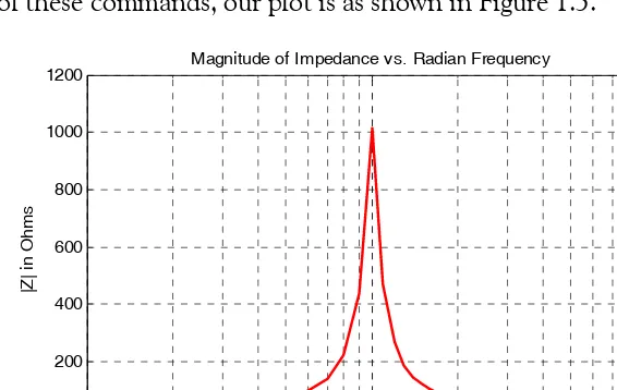
semilogx(w,z); grid; % Replaces the plot(w,z) command title('Magnitude of Impedance vs. Radian Frequency'); xlabel('w in rads/sec'); ylabel('|Z| in Ohms')

After execution of these commands, our plot is as shown in Figure 1.3.

Figure 1.3. Modified frequency response plot of Figure 1.2.

If the −axis represents power, voltage, or current, the −axis of the frequency response is more often shown in a logarithmic scale, and the −axis in dB (decibels) scale. A review of the decibel unit follows.

x y

x

x y

y x

102 103 104

0 200 400 600 800 1000

1200 Magnitude of Impedance vs. Radian Frequency

w in rads/sec

|Z

| i

n

O

h

m

s

y x

Using MATLAB to Make Plots

The ratio of any two values of the same quantity (power, voltage, or current) can be expressed in decibels (dB). Thus, we say that an amplifier has power gain, or a transmission line has a power loss of (or gain ). If the gain (or loss) is the output is equal to the input. By definition,

(1.10)

Therefore,

represents a power ratio of

represents a power ratio of

It is very useful to remember that:

represents a power ratio of

represents a power ratio of

represents a power ratio of

Also,

represents a power ratio of approximately

represents a power ratio of approximately

represents a power ratio of approximately

From these, we can estimate other values. For instance,

and since and

then,

Likewise, and this is equivalent to a power ratio of approximately

Using the relations

and

if we let , the dB values for voltage and current ratios become 10 dB

7 dB –7 dB 0 dB

dB 10 Pout

P_in ---log =

10 dB 10

10n dB 10n

20 dB 100

30 dB 1 000,

60 dB 1 000 000, ,

1 dB 1.25

3 dB 2

7 dB 5

4 dB = 3 dB+1 dB 3 dB power ratio of 2≅ 1 dB power ratio of 1.25≅

4 dB ratio of 2 1.25≅ ( × ) = ratio of 2.5

27 dB = 20 dB+7 dB 100 5× = 500

y = logx2 = 2logx

P V

2

Z

--- I2Z

= =

Chapter 1 Introduction to MATLAB

(1.11)

and

(1.12)

To display the voltage in a dB scale on the , we add the relation dB=20*log10(v), and we replace thesemilogx(w,z) command with semilogx(w,dB).

The command gtext(‘string’) switches to the current Figure Window, and displays a cross−hair which can be moved around with the mouse. For instance, we can use the command gtext(‘Impedance |Z| versus Frequency’), and this will place a cross−hair in the Figure window. Then, using the mouse, we can move the cross−hair to the position where we want our label to begin, and we press <enter>.

The command text(x,y,’string’) is similar to gtext(‘string’). It places a label on a plot in some spe-cific location specified by x and y, and string is the label which we want to place at that location. We will illustrate its use with the following example which plots a 3−phase sinusoidal waveform.

The first line of the script below has the form

linspace(first_value, last_value, number_of_values)

This command specifies the number of data points but not the increments between data points. An alternate command uses the colon notation and has the format

x=first: increment: last

This format specifies the increments between points but not the number of data points.

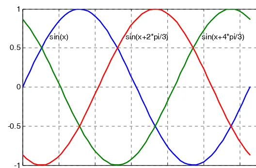
The script for the 3−phase plot is as follows:

x=linspace(0, 2*pi, 60); % pi is a built−in function in MATLAB; % we could have used x=0:0.02*pi:2*pi or x = (0: 0.02: 2)*pi instead; y=sin(x); u=sin(x+2*pi/3); v=sin(x+4*pi/3);

plot(x,y,x,u,x,v); % The x−axis must be specified for each function grid on, box on, % turn grid and axes box on

text(0.75, 0.65, 'sin(x)'); text(2.85, 0.65, 'sin(x+2*pi/3)'); text(4.95, 0.65, 'sin(x+4*pi/3)')

These three waveforms are shown on the same plot of Figure 1.4.

In our previous examples, we did not specify line styles, markers, and colors for our plots. However, MATLAB allows us to specify various line types, plot symbols, and colors. These, or a combination of these, can be added with the plot(x,y,s) command, where s is a character string containing one or more characters shown on the three columns of Table 1.2.

MATLAB has no default color; it starts with blue and cycles through the first seven colors listed in Table 1.2 for each additional line in the plot. Also, there is no default marker; no markers are

dB_v 10 Vout

V_in --- 2

log 20 Vout

V_in ---log

= =

dB_i 10 Iout

I_in --- 2

log 20 Iout

I_in ---log

= =

Using MATLAB to Make Plots

drawn unless they are selected. The default line is the solid line.

Figure 1.4. Three−phase waveforms

For example, the command plot(x,y,'m*:') plots a magenta dotted line with a star at each data point, and plot(x,y,'rs') plots a red square at each data point, but does not draw any line because no line was selected. If we want to connect the data points with a solid line, we must type plot(x,y,'rs−'). For additional information we can type help plot in MATLAB’s command screen.

TABLE 1.2 Styles, colors, and markets used in MATLAB

Symbol Color Symbol Marker Symbol Line Style

b blue . point − solid line

g green o circle : dotted line

r red x x−mark −. dash−dot line

c cyan + plus −− dashed line

m magenta * star

y yellow s square

k black d diamond

w white ⁄ triangle down

Ÿ triangle up

< triangle left

> triangle right

p pentagram

h hexagram

0 1 2 3 4 5 6 7

-1 -0.5 0 0.5 1

Chapter 1 Introduction to MATLAB

The plots which we have discussed thus far are two−dimensional, that is, they are drawn on two axes. MATLAB has also a three−dimensional (three−axes) capability and this is discussed next.

The command plot3(x,y,z)plots a line in 3−space through the points whose coordinates are the elements of , , and , where , , and are three vectors of the same length.

The general format is plot3(x₁,y₁,z₁,s₁,x₂,y₂,z₂,s₂,x₃,y₃,z₃,s₃,...) where x_n, y_n, and z_n are vectors or matrices, and s_n are strings specifying color, marker symbol, or line style. These strings are the same as those of the two−dimensional plots.

Example 1.11

Plot the function

(1.13) Solution:

We arbitrarily choose the interval (length) shown with the script below.

x= −10: 0.5: 10; % Length of vector x

y= x; % Length of vector y must be same as x

z= −2.*x.^3+x+3.*y.^2−1; % Vector z is function of both x and y* plot3(x,y,z); grid

The three−dimensional plot is shown in Figure 1.5.

Figure 1.5. Three dimensional plot for Example 1.11

* This statement uses the so called dot multiplication, dot division, and dot exponentiation where these operations are preceded by a dot (period). These operations will be explained in Section 1.8, Page 1−19.

x y z x y z

z = –2x3+ +x 3y2–1

-10 -5

0 5

10

Using MATLAB to Make Plots

The command plot3(x,y,z,'bd−') will display the plot in blue diamonds, connected with a solid line.

In a three−dimensional plot, we can use the zlabel(‘string’) command in addition to the xla-bel(‘string’) and ylaxla-bel(‘string’).

In a two−dimensional plot, we can set the limits of the − and − axes with the axis([xmin xmax ymin ymax])command. Likewise, in a three−dimensional plot we can set the limits of all three axes with the axis([xmin xmax ymin ymax zmin zmax]) command. It must be placed after the plot(x,y)orplot3(x,y,z) commands, or on the same line without first executing the plot command. This must be done for each plot. The three−dimensional text(x,y,z,’string’) command will place string beginning at the co−ordinate ( ) on the plot.

For three−dimensional plots, grid on and box off are the default states.

The mesh(x,y,z) command displays a three−dimensional plot. Another command, contour(Z,n), draws contour lines for n levels. We can also use the mesh(x,y,z) commandwith two vector argu-m e n t s . T h e s e argu-m u s t b e d e f i n e d a s a n d w h e r e

. In this case, the vertices of the mesh lines are the triples . We observe that x corresponds to the columns of , and y corresponds to the rows of .

To produce a mesh plot of a function of two variables, say , we must first generate the and matrices which consist of repeated rows and columns over the range of the variables and . We can generate the matrices and with the [X,Y]=meshgrid(x,y) function which creates the matrix whose rows are copies of the vector x, and the matrix whose columns are copies of the vector y.

Example 1.12

The volume of a right circular cone of radius and height is given by

(1.14)

Plot the volume of the cone as and vary on the intervals and meters.

Solution:

The volume of the cone is a function of both the radius and the height , that is,

The three−dimensional plot is created with the following MATLAB script where, as in the previ-ous example, in the second line we have used the dot multiplication, division, and exponentia-tion. As mentioned in the footnote of the previous page, this topic will be explained in Section 1.8, Page 1−19.

x y

x y z, ,

length x( ) = n length y( ) = m m n,

[ ] = size Z( ) {x j( ),y i( ),Z i j( ), }

Z Z

z = f x y( , )

X Y x

y X Y

X Y

V r h

V 1

3 --πr2h =

r h 0 r 4≤ ≤ 0 h 6≤ ≤

Chapter 1 Introduction to MATLAB

[R,H]=meshgrid(0: 4, 0: 6); % Creates R and H matrices from vectors r and h V=(pi .* R .^ 2 .* H) ./ 3; mesh(R, H, V)

xlabel('x−axis, radius r (meters)'); ylabel('y−axis, altitude h (meters)');

zlabel('z−axis, volume (cubic meters)'); title('Volume of Right Circular Cone'); box on

The three−dimensional plot of Figure 1.6, shows how the volume of the cone increases as the radius and height are increased.

Figure 1.6. Volume of a right circular cone.

This, and the plot of Figure 1.5, are rudimentary; MATLAB can generate very sophisticated and impressive three−dimensional plots. The MATLAB User’s manual contains more examples.

1.7 Subplots

MATLAB can display up to four windows of different plots on the Figure window using the com-mand subplot(m,n,p). This comcom-mand divides the window into an matrix of plotting areas and chooses the area to be active. No spaces or commas are required between the three inte-gers , , and . The possible combinations are shown in Figure 1.7.

We will illustrate the use of the subplot(m,n,p) command following the discussion on multiplica-tion, division and exponentiation that follows.

0 1

2 3

4

0 2

4 6

0 50 100 150

x-axis, radius r (meters) Volume of Right Circular Cone

y-axis, altitude h (meters)

z

-ax

is

, v

o

lu

m

e

(c

ubi

c

m

e

te

rs

)

m n× pth

Multiplication, Division and Exponentiation

Figure 1.7. Possible subpot arrangements in MATLAB

1.8 Multiplication, Division and Exponentiation

MATLAB recognizes two types of multiplication, division, and exponentiation. These are the matrix multiplication, division, and exponentiation, and the element−by−element multiplication, division, and exponentiation. They are explained in the following paragraphs.

In Section 1.2, the arrays , such a those that contained the coefficients of polynomi-als, consisted of one row and multiple columns, and thus are called row vectors. If an array has one column and multiple rows, it is called a column vector. We recall that the elements of a row vector are separated by spaces. To distinguish between row and column vectors, the elements of a column vector must be separated by semicolons. An easier way to construct a column vector, is to write it first as a row vector, and then transpose it into a column vector. MATLAB uses the single quotation character (¢) to transpose a vector. Thus, a column vector can be written either as

b=[−1; 3; 6; 11]

or as

b=[−1 3 6 11]'

MATLAB produces the same display with either format as shown below.

b=[−1; 3; 6; 11]

b = -1 3 6 11

b=[−1 3 6 11]'

b = -1 3

111

Full Screen Default

211 212

221 222

223 224 121 122

221 222 212

211 223 224

221

223 122 121 222 224

a b c …

Chapter 1 Introduction to MATLAB

6 11

We will now define Matrix Multiplication and Element−by−Element multiplication.

1. Matrix Multiplication (multiplication of row by column vectors) Let

and

be two vectors. We observe that is defined as a row vector whereas is defined as a column vector, as indicated by the transpose operator (′). Here, multiplication of the row vector by the column vector , is performed with the matrix multiplication operator (*). Then,

(B.15)

For example, if

and

the matrix multiplication produces the single value 68, that is,

and this is verified with the MATLAB script

A=[1 2 3 4 5]; B=[ −2 6 −3 8 7]'; A*B % Observe transpose operator (‘) in B

ans =

68

Now, let us suppose that both and are row vectors, and we attempt to perform a row−by− row multiplication with the following MATLAB statements.

A=[1 2 3 4 5]; B=[−2 6 −3 8 7]; A*B % No transpose operator (‘) here

When these statements are executed, MATLAB displays the following message:

??? Error using ==> *

Inner matrix dimensions must agree.

Here, because we have used the matrix multiplication operator (*) in A*B, MATLAB expects A = [a1 a2 a3 … an]

B = [b1 b2 b3 … bn]'

A B

A B

A*B = [a1b1+a2b2+a3b3+…+anbn] = single value

A = [1 2 3 4 5]

B = [–2 6 3– 8 7]' A*B

A∗B = 1×( )–2 +2×6+3×( )–3 +4×8+5×7 = 68

Multiplication, Division and Exponentiation

vector to be a column vector, not a row vector. It recognizes that is a row vector, and warns us that we cannot perform this multiplication using the matrix multiplication operator (*). Accordingly, we must perform this type of multiplication with a different operator. This operator is defined below.

2. Element−by−Element Multiplication (multiplication of a row vector by another row vector) Let

and

be two row vectors. Here, multiplication of the row vector by the row vector is per-formed with the dot multiplication operator (.*). There is no space between the dot and the multiplication symbol. Thus,

(B.16) This product is another row vector with the same number of elements, as the elements of and .

As an example, let

and

Dot multiplication of these two row vectors produce the following result.

Check with MATLAB:

C=[1 2 3 4 5]; % Vectors C and D must have D=[−2 6 −3 8 7]; % same number of elements

C.*D % We observe that this is a dot multiplication

ans =

-2 12 -9 32 35

Similarly, the division (/) and exponentiation (^) operators, are used for matrix division and exponentiation, whereas dot division (./) and dot exponentiation (.^) are used for element−

by−element division and exponentiation, as illustrated with the examples above.

We must remember that no space is allowed between the dot (.) and the multiplication (*), division ( /), and exponentiation (^) operators.

Note: A dot (.) is never required with the plus (+) and minus (−) operators.

B B

C = [c1 c2 c3 … cn]

D = [d1 d2 d3 … dn]

C D

C.∗D = [c1d1 c2d2 c3d3 … cndn]

C D

C = [1 2 3 4 5]

D = [–2 6 3– 8 7]

Chapter 1 Introduction to MATLAB

Example 1.13

Write the MATLAB script that produces a simple plot for the waveform defined as

(1.17)

in the seconds interval.

Solution:

The MATLAB script for this example is as follows:

t=0: 0.01: 5; % Define t−axis in 0.01 increments y=3 .* exp(−4 .* t) .* cos(5 .* t)−2 .* exp(−3 .* t) .* sin(2 .* t) + t .^2 ./ (t+1); plot(t,y); grid; xlabel('t'); ylabel('y=f(t)'); title('Plot for Example 1.13')

Figure 1.8 shows the plot for this example.

Figure 1.8. Plot for Example 1.13

Had we, in the example above, defined the time interval starting with a negative value equal to or less than , say as , MATLAB would have displayed the following message:

Warning: Divide by zero.

This is because the last term (the rational fraction) of the given expression, is divided by zero when . To avoid division by zero, we use the special MATLAB function eps, which is a number approximately equal to . It will be used with the next example.

The command axis([xmin xmax ymin ymax]) scales the current plot to the values specified by the arguments xmin, xmax, ymin and ymax. There are no commas between these four argu-ments. This command must be placed after the plot command and must be repeated for each plot.

The following example illustrates the use of the dot multiplication, division, and exponentiation, the eps number, the axis([xmin xmax ymin ymax]) command, and also MATLAB’s capability of

y f t( ) 3e–4tcos5t–2e–3tsin2t t

2

t+1 ---+

= =

0 t 5≤ ≤

0 1 2 3 4 5

-2 0 2 4 6

t

y=f

(t)

Plot for Example 1.13

1

– –3 t 3≤ ≤

t = –1

Multiplication, Division and Exponentiation

displaying up to four windows of different plots.

Example 1.14

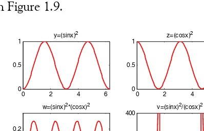
Plot the functions

(1.18)

in the interval using 100 data points. Use the subplotcommand to display these func-tions on four windows on the same graph.

Solution:

The MATLAB script to produce the four subplots is as follows:

x=linspace(0, 2*pi,100); % Interval with 100 data points y=(sin(x) .^ 2); z=(cos(x) .^ 2);

w=y .* z;

v=y ./ (z+eps); % add eps to avoid division by zero

subplot(221); % upper left of four subplots

plot(x,y); axis([0 2*pi 0 1]); title('y=(sinx)^2');

subplot(222); % upper right of four subplots

plot(x,z); axis([0 2*pi 0 1]); title('z=(cosx)^2');

subplot(223); % lower left of four subplots

plot(x,w); axis([0 2*pi 0 0.3]); title('w=(sinx)^2*(cosx)^2');

subplot(224); % lower right of four subplots

plot(x,v); axis([0 2*pi 0 400]); title('v=(sinx)^2/(cosx)^2');

These subplots are shown in Figure 1.9.

Figure 1.9. Subplots for the functions of Example 1.14

y = sin2x, z = cos2x, w = sin2x⋅ cos2x, v = sin2x⁄cos2x

0 x 2≤ ≤ π

0 2 4 6

0 0.5

1 y=(sinx)

2

0 2 4 6

0 0.5

1 z=(cosx)

2

0 2 4 6

0 0.1 0.2

w=(sinx)2*(cosx)2

0 2 4 6

0 200

400 v=(sinx)

Chapter 1 Introduction to MATLAB

The next example illustrates MATLAB’s capabilities with imaginary numbers. We will introduce the real(z) and imag(z) functions which display the real and imaginary parts of the complex quan-tity z = x + iy, the abs(z), and the angle(z) functions that compute the absolute value (magni-tude) and phase angle of the complex quantity . We will also use the polar(theta,r) function that produces a plot in polar coordinates, where r is the magnitude, theta is the angle in radians, and the round(n) function that rounds a number to its nearest integer.

Example 1.15

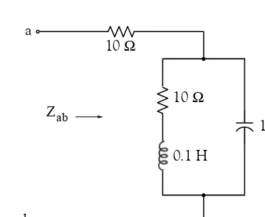
Consider the electric circuit of Figure 1.10.

Figure 1.10. Electric circuit for Example 1.15

With the given values of resistance, inductance, and capacitance, the impedance as a function of the radian frequency can be computed from the following expression.

(1.19)

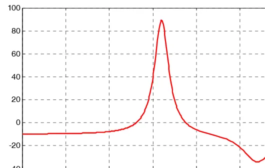
a. Plot (the real part of the impedance ) versus frequency .

b. Plot (the imaginary part of the impedance ) versus frequency .

c. Plot the impedance versus frequency in polar coordinates.

Solution:

The MATLAB script below computes the real and imaginary parts of that is, for simplicity, denoted as , and plots these as two separate graphs (parts a & b). It also produces a polar plot (part c).

w=0: 1: 2000; % Define interval with one radian interval

z=(10+(10 .^ 4 −j .* 10 .^ 6 ./ (w+eps)) ./ (10 + j .* (0.1 .* w −10.^5./ (w+eps))));

z = x+iy = r–θ

a

b

10 Ω

10 Ω

0.1 H

10 μF Z_ab

Zab

ω

Z_ab Z 10 10

4

j 10( 6⁄w)

–

10+j 0.1( w–105⁄w ) ---+

= =

Re{ }Z Z ω

Im{ }Z Z ω

Z ω

Multiplication, Division and Exponentiation

%

% The first five statements (next two lines) compute and plot Re{z} real_part=real(z); plot(w,real_part); grid;

xlabel('radian frequency w'); ylabel('Real part of Z'); %

% The next five statements (next two lines) compute and plot Im{z} imag_part=imag(z); plot(w,imag_part); grid;

xlabel('radian frequency w'); ylabel('Imaginary part of Z');

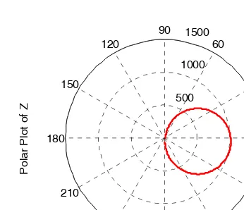
% The last six statements (next six lines) below produce the polar plot of z mag=abs(z);% Computes |Z|

rndz=round(abs(z));% Rounds |Z| to read polar plot easier theta=angle(z);% Computes the phase angle of impedance Z polar(theta,rndz);% Angle is the first argument

grid;

ylabel('Polar Plot of Z');

The real, imaginary, and polar plots are shown in Figures 1.11, 1.12, and 1.13 respectively.

Figure 1.11. Plot for the real part of Z in Example 1.15

0 200 400 600 800 1000 1200 1400 1600 1800 2000

0 200 400 600 800 1000 1200

radian frequency w

R

eal

pa

rt

of

Chapter 1 Introduction to MATLAB

Figure 1.12. Plot for the imaginary part of Z in Example 1.15

Figure 1.13. Polar plot of Z in Example 1.15

Example 1.15 clearly illustrates how powerful, fast, accurate, and flexible MATLAB is.

1.9 Script and Function Files

MATLAB recognizes two types of files: script files and function files. Both types are referred to as m−files since both require the .m extension.

A script file consists of two or more built−in functions such as those we have discussed thus far. Thus, the script for each of the examples we discussed earlier, make up a script file. Generally, a script file is one which was generated and saved as an m−file with an editor such as the MATLAB’s

0 200 400 600 800 1000 1200 1400 1600 1800 2000

-600 -400 -200 0 200 400 600

radian frequency w

Im

a

g

inary

part

o

f Z

500 1000

1500

30

210

60

240

90

270 120

300 150

330

180 0

Po

la

r Pl

o

t o

Script and Function Files

Editor/Debugger.

A function file is a user−defined function using MATLAB. We use function files for repetitive tasks. The first line of a function file must contain the word function, followed by the output argu-ment, the equal sign ( = ), and the input argument enclosed in parentheses. The function name and file name must be the same, but the file name must have the extension .m. For example, the function file consisting of the two lines below

function y = myfunction(x) y=x .^ 3 + cos(3 .* x)

is a function file and must be saved. To save it, from the File menu of the command window, we choose New and click on M−File. This takes us to the Editor Window where we type these two lines and we save it as myfunction.m.

We will use the following MATLAB functions with the next example.

The function fzero(f,x) tries to find a zero of a function of one variable, where f is a string con-taining the name of a real−valued function of a single real variable. MATLAB searches for a value near a point where the function f changes sign, and returns that value, or returns NaN if the search fails.

Important: We must remember that we use roots(p) to find the roots of polynomials only, such as those in Examples 1.1 and 1.2.

fplot(fcn,lims) − plots the function specified by the string fcn between the x−axis limits specified by lims = [xmin xmax]. Using lims = [xmin xmax ymin ymax] also controls the y−axis limits. The string fcn must be the name of an m−file function or a string with variable .

NaN (Not−a−Number) is not a function; it is MATLAB’s response to an undefined expression such as , , or inability to produce a result as described on the next paragraph.We can avoid division by zero using the eps number, which we mentioned earlier.

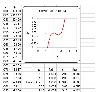
Example 1.16

Find the zeros, maxima and minima of the function

(1.20)

in the interval

Solution:

We first plot this function to observe the approximate zeros, maxima, and minima using the fol-lowing script:

x

0 0⁄ ∞ ∞⁄

f x( ) 1

x 0.1–

( )2

0.01 +

--- 1 x 1.2–

( )2

0.04 +

--- 10– +

=

1.5≤ ≤x 1.5

Chapter 1 Introduction to MATLAB

x=−1.5: 0.01: 1.5;

y=1./ ((x−0.1).^ 2 + 0.01) −1./ ((x−1.2).^ 2 + 0.04) −10; plot(x,y); grid

The plot is shown in Figure 1.14.

Figure 1.14. Plot for Example 1.16 using the plot command

The roots (zeros) of this function appear to be in the neighborhood of and . The maximum occurs at approximately where, approximately, , and the minimum occurs at approximately where, approximately, .

Next, we define and save f(x) as the funczero01.m function m−filewith the following script:

function y=funczero01(x)

% Finding the zeros of the function shown below y=1/((x−0.1)^2+0.01)−1/((x−1.2)^2+0.04)−10;

To save this file, from the File drop menu on the Command Window, we choose New, and when the Editor Window appears, we type the script above and we save it as funczero01. MATLAB appends the extension .m to it.

Now, we can use the fplot(fcn,lims) command to plot as follows:

fplot('funczero01', [−1.5 1.5]); grid

This plot is shown in Figure 1.15. As expected, this plot is identical to the plot of Figure 1.14 which was obtained with the plot(x,y) command as shown in Figure 1.14.

-1.5 -1 -0.5 0 0.5 1 1.5

-40 -20 0 20 40 60 80 100

x = –0.2 x = 0.3

x = 0.1 y_max = 90

x = 1.2 y_min = –34

Script and Function Files

Figure 1.15. Plot for Example 1.16 using the fplot command

We will use the fzero(f,x) function to compute the roots of in Equation (1.20) more pre-cisely. The MATLAB script below will accomplish this.

x1= fzero('funczero01', −0.2); x2= fzero('funczero01', 0.3);

fprintf('The roots (zeros) of this function are r1= %3.4f', x1); fprintf(' and r2= %3.4f \n', x2)

MATLAB displays the following:

The roots (zeros) of this function are r1= -0.1919 and r2= 0.3788

The earlier MATLAB versions included the function fmin(f,x1,x2) and with this function we could compute both a minimum of some function or a maximum of since a maximum of is equal to a minimum of . This can be visualized by flipping the plot of a function upside−down. This function is no longer used in MATLAB and thus we will compute the maxima and minima from the derivative of the given function.

From elementary calculus, we recall that the maxima or minima of a function can be found by setting the first derivative of a function equal to zero and solving for the independent variable . For this example we use the diff(x) function which produces the approximate deriva-tive of a function. Thus, we use the following MATLAB script:

syms x ymin zmin; ymin=1/((x−0.1)^2+0.01)−1/((x−1.2)^2+0.04)−10;... zmin=diff(ymin)

zmin =

-1/((x-1/10)^2+1/100)^2*(2*x-1/5)+1/((x-6/5)^2+1/25)^2*(2*x-12/5)

When the command

-1.5 -1 -0.5 0 0.5 1 1.5

-40 -20 0 20 40 60 80 100

f x( )

f x( ) f x( )

f x( ) –f x( )

f x( )

y = f x( )

Chapter 1 Introduction to MATLAB

solve(zmin)

is executed, MATLAB displays a very long expression which when copied at the command prompt and executed, produces the following:

ans =

0.6585 + 0.3437i ans =

0.6585 - 0.3437i ans =

1.2012

The real value above is the value of at which the function has its minimum value as we observe also in the plot of Figure 1.15.

To find the value of y corresponding to this value of x, we substitute it into , that is,

x=1.2012; ymin=1 / ((x−0.1) ^ 2 + 0.01) −1 / ((x−1.2) ^ 2 + 0.04) −10

ymin = -34.1812

We can find the maximum value from whose plot is produced with the script

x=−1.5:0.01:1.5; ymax=−1./((x−0.1).^2+0.01)+1./((x−1.2).^2+0.04)+10; plot(x,ymax); grid

and the plot is shown in Figure 1.16.

Figure 1.16. Plot of for Example 1.16

Next we compute the first derivative of and we solve for to find the value where the max-imum of occurs. This is accomplished with the MATLAB script below.

syms x ymax zmax; ymax=−(1/((x−0.1)^2+0.01)−1/((x−1.2)^2+0.04)−10); zmax=diff(ymax)

1.2012 x y

f x( )

f x( )

–

-1.5 -1 -0.5 0 0.5 1 1.5

-100 -80 -60 -40 -20 0 20 40

f x( )

–

f x( )

– x

Display Formats

zmax =

1/((x-1/10)^2+1/100)^2*(2*x-1/5)-1/((x-6/5)^2+1/25)^2*(2*x-12/5)

solve(zmax)

When the command

solve(zmax)

is executed, MATLAB displays a very long expression which when copied at the command prompt and executed, produces the following:

ans =

0.6585 + 0.3437i

ans =

0.6585 - 0.3437i

ans =

1.2012 ans =

0.0999

From the values above we choose which is consistent with the plots of Figures 1.15 and 1.16. Accordingly, we execute the following script to obtain the value of .

x=0.0999; % Using this value find the corresponding value of ymax

ymax=1 / ((x−0.1) ^ 2 + 0.01) −1 / ((x−1.2) ^ 2 + 0.04) −10

ymax = 89.2000

1.10 Display Formats

MATLAB displays the results on the screen in integer format without decimals if the result is an integer number, or in short floating point format with four decimals if it a fractional number. The format displayed has nothing to do with the accuracy in the computations. MATLAB performs all computations with accuracy up to 16 decimal places.

The output format can changed with the format command. The available formats can be displayed with the help format command as follows:

help format

FORMAT Set output format.

All computations in MATLAB are done in double precision.

FORMAT may be used to switch between different output display formats as follows:

x = 0.0999

Chapter 1 Introduction to MATLAB

FORMAT Default. Same as SHORT.

FORMAT SHORT Scaled fixed point format with 5 digits. FORMAT LONG Scaled fixed point format with 15 digits. FORMAT SHORT E Floating point format with 5 digits.

FORMAT LONG E Floating point format with 15 digits. FORMAT SHORT G Best of fixed or floating point

format with 5 digits.

FORMAT LONG G Best of fixed or floating point format with 15 digits.

FORMAT HEX Hexadecimal format.

FORMAT + The symbols +, - and blank are printed for positive, negative and zero elements. Imaginary parts are ignored.

FORMAT BANK Fixed format for dollars and cents.

FORMAT RAT Approximation by ratio of small integers.

Spacing:

FORMAT COMPACT Suppress extra line-feeds.

FORMAT LOOSE Puts the extra line-feeds back in.

Some examples with different format displays age given below.

format short 33.3335 Four decimal digits (default)

format long 33.33333333333334 16 digits

format short e 3.3333e+01 Four decimal digits plus exponent

format short g 33.333 Better of format short or format short e

format bank 33.33 two decimal digits

format + only + or − or zero are printed

Summary

1.11 Summary

• We can get help with MATLAB topics by typing help followed by any topic available. For example, the command help matlab\iofun will display input/output information, and help mat-lab graphicswill display help on graphics.

• The MATLAB Demos menu displays MATLAB’s capabilities. To access it, we type demo and we see the different topics. Whenever we want to return to the command window, we click on the Close button.

• We type quit or exit when we are done and want to leave MATLAB.

• We use the clear command if we want to clear all previous values, variables, and equations without exiting.

• The clc command clears the screen but MATLAB still remembers all values, variables and equations which we have already used.

• All text after the % (percent) symbol is interpreted by MATLAB as a comment line and thus it is ignored during the execution of a program. A comment can be typed on the same line as the function or command or as a separate line.

• For computations involving complex numbers we can use either , or to denote the imagi-nary part of the complex number.

• In MATLAB, a polynomial is expressed as a row vector of the form . The elements of this vector are the coeffic