Noise Removal from Medical Images Using Shrinkage Based Enhanced Total Variation Technique

Noise Removal from Medical Images Using

Shrinkage Based Enhanced Total Variation

Technique

Devanand Bhonsle, Department of EEE, Shri Shankaracharya Technical Campus, Bhilai, India. E-mail:devanandbhonsle@gmail.com

Vivek Kumar Chandra, Department of EEE, Chhatrapati Shivaji Institute of Technology-Durg, India. E-mail:vivekchanda1@rediffmail.com

G.R. Sinha, Department of ECE, CMR Technical Campus, Hydrabad, India. E-mail:drgrsinha@ieee.org

Abstract---Generally the acquisition procedure, there may perhaps be distortions in the images, which will impact negatively the diagnosis images. Suggests a new mixed noise removal algorithm by combining two spatial filters and shrinkage combined enhanced total variation (SCETV) technique. By introducing the CT-Scan image, which is an impulse novel method of de-noising is proposed. The Operation was accomplished in two phases: receiving reference image and also image de-noising. We introduce the adaptive trilateral filter for combined noise rejection for de-noising and lastly we combine them with Shrinkage combined total variation method in which images are approved through bivariate shrinkage and the Enhanced total variation techniques in parallel. Then the two images attained from the SCETV technique is fused utilizing Dual Tree Complex Wavelet Transform (DTCWT). The consequential noiseless fused images are subjected to image restoration procedure by efficiently employing the hybridized form of KH algorithm and Richardson-Lucy (RL) approach. The cheering performance outcomes chant the triumph stories of the novel image restoration method, highlighting its superlative efficiency and the suggested approach achieves great results both regarding quantitative measures of signal restoration and qualitative judgments of image quality. Moreover, the computational intricacy of the suggested methodology is lesser than that of several other combined noise filters.

Keywords---Acquisition, Shrinkage, Total Variation, De-noising and Image Restoration.

I.

Introduction

Medical imaging has been the method and procedure of generating the inner of a body’s visual representations for clinical evaluation besides medical intervention, and visual representation in the role of few organs or else tissues (physiology). Medical imaging searches for enlightening internal structures concealed through the skin with bones, and for diagnosing and treating disease. Also, Medical imaging confirms a data warehouse of normal anatomy database and physiology for making it possible for recognizing abnormalities [1]. Medical imaging approaches, like computed tomography (CT) plus Magnetic Resonance Imaging (MRI) has a vital part in the medical clinical investigation and disease diagnosis. However, by reason of the technique limitation, the random noise often degrades the acquired medical images’ quality, which seriously affects the medical image scrutiny [2]. Image noise represents unwanted information which may influence the image quality. It is generally an electronic noise appearance which contains a haphazard variation of colour or else brightness in images [3]. Noise existing in medical images may affect the diagnosis outcome of the patient, which emphasizes the significance of noise lessening for deteriorated medical images [4].

derive the de-noised image through an inverse transform [12]. Image renovation is the work of reducing the degradation of an image i.e. recuperating an image that worsened as a consequence of the noise present. Image restoration methodology augments image quality through discarding noisy pixels. The renovation of the really tainted image is completed by scripting algorithms that proceed to recognize a noisy pixel in a complete image [13].

II.

Related Work

Barcelos et al. [14] have suggested an innovative variational technique for the rebuilding of images degraded through the non-uniformly distributed noise. Here, the model comprised a balance betwixt the data term plus the regularization term in energy functional, that considered the statistical power of parameters plus the noisy points’ position associated with the edges given in image. Moreover, the parameters were resolved by the provided preliminary noisy image. The derived outcomes presented the efficacy and powerfulness of the suggested model and in renovating images with multiplicative noise or else combined Gaussian noise, while conserving edges and also undersized structures held by the image.

Phophalia et al. [15] have suggested a rough set theory (RST) related technique that was utilized for obtaining pixel equal edge map plus class labels that in turn were utilized for enhancing the bilateral filters’ performance. RST manages the vagueness prevailed in the data even under the noise. The basic structure of the bilateral filter was not much amended, anyhow, enhanced up through prior information attained from rough edge map plus rough class labels. The filter was applied extensively for de-noising the brain MR images.

P.R. Hill et al. [16] have suggested two un-decimated procedures of Dual Tree Complex Wavelet Transform (DT-CWT) to the application for image de-noising plus effective extraction of the feature. Such un-decimated transforms expand the DT-CWT by the exclusion of down sampling of filter outputs combined with up sampling of the intricacy filter pairs in a similar formation to Un-decimated Discrete Wavelet Transform (UDWT). Both the established transforms proffered same translational invariance, enhanced scale-to-scale coefficient correlation accompanied by the directional selectivity of the DT-CWT. Moreover, amidst every improved transform, sub bands were having a constant size. Therefore they derived benefit from a straight one-to-one relationship betwixt co-located coefficients in every scale and thence this provides constant phase relationships through scales. Such benefits were used amidst applications of denoising, image fusion, over and above robust feature extraction with segmentation.

Cheolkon Jung et al. [17] have conferred function of a logarithmic for global brightness development as stated by the nonlinear reaction of human vision to scintillating. Furthermore, developed the local difference via contrast limited adaptive histogram equalization (CLAHE) in minimal-pass sub bands intended for making image structure more lucid. Regarding noise reduction, as stated by the direction choosy property of DT-CWT, they performed content-based total variation (TV) diffusion that limits the smoothing degree as per noise plus edges in great-pass sub bands. Evaluation outcomes elucidated that the technique attains an enhanced performance in minimal light image development and outperforms cutting edge ones regarding contrast development and also noise reduction.

Hao-Liang Yang et al. [18] have proposed an innovative blind image convolution algorithm for motion de-blurring by a single blurred image. They have suggested a combined framework for blur kernel evaluation and also non-blind image convolution through utilization bilateral filtering (BF) and also an innovative image de-convolution algorithm, named the Gradient Attenuation Richardson–Lucy (GARL) algorithm. During blur kernel evaluation stage, they presented that a first blur kernel that was utilized for commencing another kernel refinement procedure is obtained from blurred image and a quadratic regularization procedure. In the non-blind image de-convolution phase, they used the image gradients, and augment the GARL algorithm for alleviating the well-known ringing issue in the Richardson–Lucy-related image restoration method. Moreover, the image loss details on account of ringing artifacts suppression around the areas having powerful edges were improved through an incremental detail recovery process.

III.

Proposed SCETV

The innovative technique runs through the subsequent phases.

a. Preprocessing

b. SCETV De-noising Technique c. Image fusion utilizing DTCWT

A. Preprocessing

The noise represents the adverse impact generated in an image which eventually heads to the diminution of the image quality. Hence, it is still more essential to annihilate the noise from the image. Let we considered an image database

D

=

{

I

(

u

,

v

)

n

}

, where

0

≤

u

≤

M

−

1

, &

0

≤

v

≤

N

−

1

,

n

is the number of images and

I

(

u

,

v

)

T

be the image affected by the noise typeT.In this novel approach, for the reason of steering clear of the noise, three distinct and effective filters are engaged which is illustrated below.

AWGN Noise Appended to CT-Scan Image

The considered image

I

T

(

i

,

j

)

gets converted to

I

A

(

i

,

j

)

where A represents that AWGN noise is appended

to the actual image. The AWGN noise in an image

I

A

(

i

,

j

)

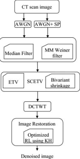
is partially removed using the amalgamation of Median Filter (MF) and Median Modified Weiner Filter (MMWF) for improved performance. Initially, the AWGN noise added image is accepted through the MF and then done by the MMWF.

Figure 1: Architectural Flow of the Suggested SCETV De-noising Technique

In noise removal, the manner of median filtering is given above in which is proceeded by the median modified Weiner filter. Once the image

I

A

(

i

,

j

)

is accepted through a median filter then the same image

I

A

(

i

,

j

)

is next accepted through the median modified Weiner filter.

MMWF (Median Modified Weiner Filter)

The MMWF concerns the local kernel mean around every pixel m. This value is substituted with the evaluation

of the local kernel median around every pixel

I

A

(

i

,

j

)

~m, considering the notation ~

µ

to indicate the local window median around every single pixel

µ

resulting in the subsequent formula.

)

)

,

(

(

)

,

(

~

2 2 2 ~

µ

σ

ν

σ

µ

+

−

−

=

I

i

j

j

i

I

_MMWF A ₍₁₎

Where

ν

2 is the noise variance in the approximation of the local (i.e. considered in sliding window) mean

µ

Thus CT-Scan image tainted with the AWGN noise is accepted through median filter along with MMWF for effective elimination of noise.

The algorithm 1for median filter to exterminate the noise appended to the image is explained as follows.

Algorithm 1: Median Filter

Mixed Noise (Salt and Pepper + AWGN) appended to CT-Scan Image

This mixed noise appended to a CT-Scan image represented by

I

T

(

i

,

j

)

after which it converts to

)

,

(

i

j

I

SA

image with the mixed noise. These noises partially are removed using the amalgamation of the Median Filter along with Median Modified Weiner Filter. The CT-Scan image corrupted with mixed noise (salt and pepper + AWGN) is accepted through the same filters median and MMWF mentioned in algorithm 1 and formula (1) in the preprocessing method.

B. SCETV De-noising Technique

The final image attained from the MMWF

I

MMWF

(

i

,

j

)

for mixed noise and the single AWGN noise added image is brought the recommended SCETV technique’s step. This proposed technique includes the amalgamation of the bivariate Shrinkage and the Enhanced Total variation technique. The images accepted through the filters are then accepted through the bivariant shrinkage and Enhanced Total Variation technique in parallel.

Bivariant Shrinkage

In [19], suggested a bivariate probability density function (pdf) for modeling the statistical dependence betwixt a coefficient and also its parent, furthermore, the associating function of bivariate shrinkage is derived. An image de-noising degraded by combined noise plus AWGN noise with variance

σ

_n2will be measured.

Let

w

_2krepresent the parent of

w

_1k formulated the issues in wavelet domain as

y

_1k

=

w

_1k

+

n

_1kand

k k

k

w

n

y

₂

=

₂

+

₂ to consider statistical dependencies betwixt a coefficient plus its parent.

y

_1k and

y

_2k have

been the noisy clarification of

w

_1k and

w

_{2k ; and}

n

_1k and

n

_2k are the noise samples. Here, it can be specified as

k k

k

w

n

y

=

+

k= 1…no. of wavelet coefs (2)

allocate output Pixel Value [image width][image height] allocate window[window width * window height] edge a := (window width / 2) rounded down edge b := (window height / 2) rounded down for a from edge a to image width – edge a for b from edge b to image height – edge b i = 0

for f(a) from 0 to window width for f(b) from 0 to window height

window[i] := input Pixel Value [a + f(a)– edge a][b + f(b) – edge b] i := i + 1

sort entries in window[]

Where

w

k

=

(

w

1k

,

w

2k

),

y

k

=

(

y

1k

,

y

2k

)

and

n

k

=

n

1k

+

n

2k_. In this regards, the coefficient index

k

will

be evicted from the expression to progress the equations’ readability. The typical MAP estimator for

w

provided the degraded observation y is

(3)

After some manipulations, this equation can be expressed as

(4)

A non-Gaussian bivariate (pdf) for the coefficient plus its parent as

).

The secondary variance 2

σ

has been also reliant on the coefficient index

k

. Utilizing (1) MAP estimator of

BI Which is illustrated as a bivariate shrinkage function. Here (g)+ is denoted as



This estimator needs the prior information of noise variance σn2plus the marginal variance 2

σ _{for every wavelet}

coefficient. The last output image in the derived bi-variant shrinkage is denoted as BI

I1 ^

.

Enhanced Total Variation

In Enhanced total variation technique the de-noising problem formulated as an optimization issue whose solution derived utilizing the split-bregman approach. To reduce mixed Gaussian and sparse noise from hyper spectral images through explicitly considering in the suggested issue formulation, hyper spectral de-noising is a well-researched issue. There are researches in which deemed mixed noise reduction from grayscale images. The enhanced total variation (ETV) model extends the traditional total variation prototype and accounts for the spatial plus the spectral correlation. The resulting optimization issue has been rectified utilizing a split-Bregman scheme. The attained images in the previous process is accepted through the TV algorithm [19, 20] which gives the subsequent image

C. Image Fusion Using DTCWT

The single image when accepted through the bi-variant shrinkage and Enhanced Total Variation technique yields two resulting images which have been the by-product of two distinct de-noising methodologies. The two de-noised

images merged together utilizing the DTCWT method. This is illustrated as DTCWT

I1

To overcome drawbacks of the standard wavelet transform have utilized Dual tree complex wavelet transform. Complex wavelet transform (CWT) is complicated valued expansion to typical DWT. CWT utilize intricate value

filtering which decomposes the actual/complex signal into imaginary and real parts in a transform domain. The imaginary and real coefficients are utilized for calculating amplitude and also phase information. DTCWT divided sub bands aimed at positive along with negative orientations. DTCWT compute the complicated transform of signal utilizing two distinct discrete wavelet transform (DWT) decomposition. DWT decomposition creates two equivalent trees.

D. The Image Restoration Using Optimized KH based RL

This technique resorts the deployment of KH method along with Richardson-Lucy (R-L) algorithm. In image restitution procedure, the all-powerful Point Spread Function (PSF) is entrusted with the chore of performing successful restitution. The optimized PSF via new-fangled KH is advantageous to the RL algorithm for restoring the

distorted image. Fused image I1DTCWT ^

is then accepted through the optimized KH based RL algorithm.

The noiseless image '

f

I

attained from the hybrid filter seems like distorted, hence it is highly essential to fine-tune the image quality. With an eye on boosting the noiseless image quality, we have resorted to the deployment of KH method along with Richardson-Lucy (R-L) algorithm. In image restitution procedure, the all-powerful Point Spread Function (PSF) is entrusted with the assignment of performing successful restitution. The optimized PSF via new-fangled KH is advantageous to the RL algorithm for restoring the distorted image. The modus operandi of KH regarding PSF calculation is detailed as follows:

STEP 1: Initially assume the entire number of population asK and iterations as

J

_mx.

STEP 2: Arbitrarily produce the initial total population value

M

_A, where A= 1, 2, 3....K individual enthalpies respectively. Establish the following parameters for the ensuing functions:

• Foraging Speed

R

_A

• Maximum induced speed

M

_max

• Optimum iteration number

J

_mx

STEP 3: Compute the fitness function through determining all individual enthalpies based on its present position.

STEP 4: Analyze the motion by considering the three elements which are mentioned below:

i) Accordance with other Total population values

Selection of the

j

th individual total population, such that

M

_jcan be defined as

old

Where,

M

max

→

_{maximum induced speed,}

old

Local effect delivered by the vicinity total population value,

→

T j

Z

Target effect delivered by the vicinity total population values.

ii) Foraging motion

best

Effect of available total population

values,

best j

µ

_→

Effect of best total population value iii) Physical diffusion

This is nothing but the random diffusion of enthalpies in the solution space. The entire population computation is estimated from the speed of enthalpies and a randomly created directional vector. The expression to compute this diffusion result of the total population is signified as follows:

(

)

_

_τ

Whereas,

S

max

→

_{Maximum diffusion speed,}

τ →

_{Random directional vector between [-1, 1]} STEP 5: Suppose, if the situation of the optimization issue is dissatisfied, then move to step 3.

STEP 6: Improve the new positions of the selected total population amongst the available total enthalpies correspondingly,

Employing all the efficient parameters (

M

j_,

R

j_,

S

j_{) of the motion attained over time, the total population’s}

random position during the interval

f

and

∆

f

can be completed by the subsequent equation and the position of the each total population value is updated. According to uniform distribution function,

(

f

+

∆

f

)

=

X

_j

( )

f

+

∆

f

.

(

dX

_j

df

)

(15)

Whereas, Δf, is termed as a Scale factor,

STEP 7: Suppose, if the termination norm is not met, then move to step3 and redo the procedure duly.

STEP 8: Else, if the termination condition is satisfied, then determine the optimum possible solution in the search space.

Richardson-Lucy Algorithm

This algorithm employs a probabilistic method for restoring the deformed image. At this time the tainted image '

f

I

is furnished as input, and an image k that maximizes the possibility of observing the image

I

_f' is discovered. Taking the image as a scrutiny of a Poisson procedure, the probability function is stated as:

∏

−

A repetitive algorithm might be resultant from the precedant functional. It is termed as the Richardson-Lucy algorithm and is furnished by:

This algorithm comes to a stop after a explicit number of iterations. When the de-convolution is ill-posed, which usually happens in real applications, the signal-to-noise ratio tends to become exceedingly inferior to a number of iterations

n

→

∞

. In RL algorithm, a set of operations is performed for permanent number of iterations and at last,

we come face to face with the expected, improved, reclaimed image '

f

I

IV.

Experimental Results and Discussion

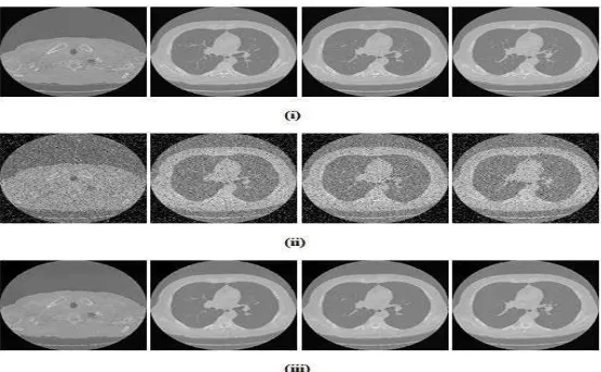
The novel heuristic method is performed in the working platform of the MATLAB version 7.14 combined with the classification GUI (Graphical User Interface) which is furnished for both the Gaussian plus salt and pepper commotion categories. The input image de-noised with the assistance of the innovative hybrid Adaptive median filter along with the adaptive fuzzy switching with the AGA technique. Further, a de-noised image is regained by the AGA (Richard-Lucy technique). The sample input images employed in the new-fangled approach are effectively exhibited in figure 2 (i) and 3(i).

Figure 1 : Images for (i) Sample Input of CT-Scan Image (ii) Gaussian Noise Added Image (iii) Gaussian Noise Removed Image

Discussion: Well-before the start of noise removal procedure, it is noticed from figure 2(ii) which indicates that Gaussian noise is appended to the input image figure 2(i). The figure 2(iii) appearing below illustrates the samples of Gaussian noise-removed images by the intended method of SCETV de-noising method. Form the figure 2(iii) it is clear that our intended method yields better performance.

Discussion: The above-illustrated figure 3(i) shows the input images utilized for the estimating our proposed SCETV de-noising technique. The noisy image in figure 3(ii) indicates the addition of combined noise (AWGN+ salt and pepper) to the input image figure 3(i). The figure 3(iii) gives the output attained after implementing the proposed SCETV de-noising method aimed at efficient mixed noise removal. The final resorted image attained describes the better effectiveness of suggested de-noising technique.

V.

Performance Analysis

The functioning of the novel method is effectively appraised with the assistance of two efficiency metrics such as SNR also PSNR by duly modulating the Gaussian and mixed noise (AWGN+ salt and pepper) on both high plus low degree of noise. In addition, graphical demonstrations are specified below for an improved apprehension of the suggested task. In this connection, the noise elimination feat of the novel method for eradicating Gaussian noise appended to the CT-Scan image is paralleled with those of the prevailing de-noising methods regarding their PSNR values are effectively furnished in Table 1.

Table 1: Proposed and Existing Filtering Methods PSNR Value of Three Different Noise Variance Levels for Gaussian Noise Appended to CT-Scan Image

AWGN Noise SNR Level

Images Noisy PSNR

Noisy SNR

RL-PSNR

RL-SNR

Proposed SCETV PSNR

Proposed SCETV SNR

5 Image 1 11.9846 6.2289 16.6326 10.8773 20.3389 14.5834

10 Image 2 16.2778 10.5223 20.1007 14.3454 24.3489 18.59363 15 Image 3 21.1548 15.3994 23.7847 18.0293 28.6424 22.88692 20 Image 4 26.0666 20.3111 26.2659 20.5105 32.0467 26.29131 25 Image 5 21.1799 15.4243 23.7301 17.9749 28.56199 22.80675

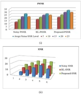
The average PSNR value computed from the above-given tables are represented as graphs in Fig. 4(i) which specifies that the PSNR for the Suggested SCETV is greater matched with variant existing RL based PSNR and 5(ii) includes the graphical delineation of the SNR values in which the Suggested SCETV shows the higher SNR value when contrasted with the Noisy SNR attained and RL based SNR.

(i)

(ii)

Table 2: Proposed and Existing Filtering Methods PSNR Value of Various Noise Variance Levels for Combined Noise Appended to CT-Scan Image

AWGN+S&P Noise Level

Images Noisy PSNR

Noisy SNR

RL-PSNR

RL-SNR

Proposed SCETV-PSNR

Proposed SCETV-SNR

High level Noise

0.01 Image 1 15.1267 9.37124 27.505 21.749 33.49764 27.7424 0.03 Image 2 10.3718 4.61578 19.706 13.951 25.35022 19.5949 0.05 Image 3 8.1609 2.40562 15.112 9.3575 19.00057 13.2453 0.07 Image 4 6.6935 0.93803 11.064 5.3093 14.14441 8.38918

0.09 Image 5 5.5955 -0.1598 5.0791 0.676 7.473514 1.71828

Low Level Noise

0.1 Image 1 15.128 9.37124 27.505 21.749 33.49764 27.7424

0.3 Image 2 10.372 4.61578 19.706 13.951 25.35022 19.5949

0.5 Image 3 8.1609 2.40562 15.112 9.3576 19.00057 13.2453

0.7 Image 4 6.6935 0.93803 11.064 5.3094 14.14441 8.38918

0.9 Image 5 5.5954 0.15988 5.0790 0.676 7.473514 1.71828

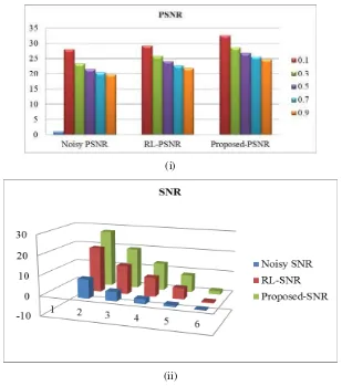
Discussion: The above given table 2 describes the mixed noise (AWGN + salt and pepper) in both high level and low levels of variance appended to a CT-Scan image. From the table, it is perceived that the PSNR for proposed SCETV is better to the existing ones, which shows the better performance of the system. Similarly, the SNR values attained for the suggested one is exceeding the existing ones. In both the cases of low plus a high level of noises the SNR along with PSNR values shows the efficacy of the deliberated method. The graphical demonstration for the precedent table values for SNR together with PSNR values are shown individually below in figure 5(i) and 5(ii). The graphs in figure 5(i) and (ii) prove the higher value of SNR accompanied by PSNR meant for the suggested SCETV method.

(i)

(ii)

Table 3: Comparison of Proposed and Existing Filtering Methods SNR and PSNR values with Various Noise Levels for Mixed Noise Appended to CT-Scan Image

Noise Level Noisy PSNR RL-PSNR Proposed-PSNR 0.1 28.07878311 29.30251586 32.67172924 0.3 23.42807629 25.93536055 28.72747042 0.5 21.5336962 24.1755801 26.93479837 0.7 20.48289611 22.79333974 25.69232173 0.9 19.82620771 21.92633278 24.6932812 High Level Noisy SNR RL-SNR Proposed-SNR 1.2 19.09525119 20.94989167 23.76061765 1.4 18.70066696 20.53388808 23.35429997 1.6 18.38773964 20.13154886 22.84918297 1.8 18.12766972 19.76665428 22.57601757 2 17.87367458 19.37642641 22.20114359

Discussion: The above-mentioned table 3 includes the SNR along with PSNR values of the suggested SCETV method and the existing RL based method for the speckle noise at both low and high noise level appended to the ultrasonic images. From the table, it is noted that the values of SNR over and above PSNR for the suggested SCETV is superior to the existing one. The graphical presentation of the table 2 is given below for the enhanced comprehension of the suggested one.

VI.

Conclusion

In the suggested image restoration technique, initially, the preprocessing is done by two filters MF and MMWF filter then that preprocessed image is provided to subsequent step of noise removal process that includes the intended method SCETV which is trailed by the dual tree complex wavelet transform technique. During noise removal procedure, parameters RL are maximized by using KH Algorithm. All this process has enhanced the noise removal performance and restoration methods. The results have provided that the suggested method has attained greater PSNR values than the prevailing maximization techniques. Thus, the suggested techniques have proffered better performance in de-noising all sort of noisy images with greater de-noising PSNR ratio and renovate all images with great quality. In future, the evaluation of speckle noise is performed utilizing the relevant type of images.

References

[1] https://en.wikipedia.org/wiki/Medical_imaging

[2] Bai, J., Sun, Y., Fan, T., Song, S. and Zhang, X. Medical image denoising based on improving K-SVD and block-matching 3D filtering. IEEE Region 10 Conference TENCON, 2016, 1624-1627.

[3] https://www.ijsr.net/archive/v3i4/MDIwMTMxNTQ2.pdf

[4] Ting, F.F., Sim, K.S. and Wong, E.K. A rapid medical image noise variance estimation method.

International Conference on Robotics, Automation and Sciences, 2016, 1-6.

[5] Sanchez, M.G., Sánchez, M.G., Vidal, V., Verdu, G., Verdú, G., Mayo, P. and Rodenas, F. Medical image restoration with different types of noise. IEEE Annual International Conference of the Engineering in Medicine and Biology Society (EMBC), 2012, 4382-4385.

[6] Mohan, M.R.M., Sulochana, C.H. and Latha, T. Medical image denoising using multistage directional median filter. International Conference on Circuit, Power and Computing Technologies, 2015, 1-6.

[7] Thakur, K., Damodare, O. and Sapkal, A. Hybrid method for medical image denoising using Shearlet transform and bilateral filter. International Conference on Information Processing, 2015, 220-224.

[8] Suresh, K.V. An improved image denoising using wavelet transform. International Conference on Trends in Automation, Communications and Computing Technology, 2015.

[9] Bhadauria, H.S. and Dewal, M.L. Medical image denoising using adaptive fusion of curvelet transform and total variation. Computers & Electrical Engineering39 (5) (2013) 1451-1460.

[10] Kazmi, M., Aziz, A., Akhtar, P., Maftun, A. and Afaq, W.B. Medical image denoising based on adaptive thresholding in contourlet domain. 5th International Conference on Biomedical Engineering and Informatics (BMEI), 2012, 313-318.

[11] Naimi, H., Adamou-Mitiche, A.B.H. and Mitiche, L. Medical image denoising using dual tree complex thresholding wavelet transform and Wiener filter. Journal of King Saud University-Computer and Information Sciences27 (1) (2015) 40-45.

[13] https://www.worldwidejournals.com/indian-journal-of-applied research (IJAR)/file.php?val=April_2015_ 1427895945__74.pdf

[14] Barcelos, C.A.Z. and Barcelos, E.Z. A well-balanced and adaptive variational model for the removal of mixed noise. Computers & Electrical Engineering40 (7) (2014) 2027-2037.

[15] Phophalia, A. and Mitra, S.K. Rough set based bilateral filter design for denoising brain MR images.

Applied Soft Computing33 (2015) 1-14.

[16] Hill, P.R., Anantrasirichai, N., Achim, A., Al-Mualla, M.E. and David R. Bull. Undecimated dual-tree complex wavelet transforms. Signal Processing: Image Communication35 (2015) 61-70.

[17] Jung, C., Yang, Q., Sun, T., Fu, Q. and Song, H. Low light image enhancement with dual-tree complex wavelet transform. Journal of Visual Communication and Image Representation42 (2017) 28-36.

[18] Yang, H.L., Huang, P.H. and Lai, S.H. A novel gradient attenuation Richardson–Lucy algorithm for image motion deblurring. Signal Processing103 (2014) 399-414.

[19] Sendur, L. and Selesnick, I.W. Bivariate shrinkage with local variance estimation. IEEE signal processing letters9 (12) (2002) 438-441.

[20] Aggarwal, H.K. and Majumdar, A. Hyperspectral image denoising using spatio-spectral total variation.