Range restricted interpolation using Gregory’s rational
cubic splines
Marion Bastian-Walther, Jochen W. Schmidt∗
Technische Universitat, Institut fur Numerische Mathematik, D-01062 Dresden, Germany
Received 16 March 1998
Abstract
The construction of range restricted univariate and bivariate interpolants to gridded data is considered. We apply Gregory’s rational cubicC1splines as well as related rational quinticC2splines. Assume that the lower and upper obstacles are compatible with the data set. Then the tension parameters occurring in the mentioned spline classes can be always determined in such a way that range restricted interpolation is successful. c1999 Elsevier Science B.V. All rights reserved.
Keywords:Interpolation subject to piecewise linear obstacles; Gregory’s splines and corresponding tensor products;
Solvability bounds to the tension parameters; Existence and construction of spline solutions
1. Introduction
Gregory’s rational cubic splines [7] are known to be very useful in univariate monotone and convex interpolation, see the paper [3] and Spath’s monograph [22] where the respective algorithms can be found, too. The present paper is devoted to the problem of range restricted interpolation being also of interest in several applications. Again, the above splines allow satisfactory numerical methods for constructing the desired interpolants. In addition, the univariate results can be extended to the interpolation of bivariate data sets given on a rectangular array. To this end tensor product techniques including the nonnegativity lemma [10, 11] are applied.
There are other types of rational splines successfully considered in convex interpolation. In par-ticular, we refer to Spath’s rational cubic splines [22, chapter 6.4]. However, it must be left as an open question whether these splines are suitable in the present constrained interpolation problem.
Recently several papers have appeared that concern with range restricted interpolation. Univariate problems are considered in [6, 9, 15, 16] using particular rational splines while the papers [1, 4, 14] are based on a variational approach. Polynomial splines on rened grids, respectively triangulations
∗Corresponding author. E-mail: [email protected].
of bivariate data sites are applied in [8, 12, 13], and [18, 19]. The latter two papers are concerned with interpolation subject to restrictions on the rst, respectively second order derivatives; a review is given in [17]. Finally, we mention the papers [5, 20, 21] which deal with univariate range restricted least squares smoothing.
For comparisons we outline the present direct method in some more details. Starting from the concrete class of Gregory’s rational cubic C1 splines, in the rst step we derive sucient conditions for the fulllment of the range restrictions. These are inequalities with respect to derivative parameters and to the tension parameters; see (15) for a univariate example and (49) for a bivariate one. Because the interpolation conditions as well as the smoothness requirements are incorporated into the spline representation, the solvability of the range restricted interpolation problems depends only on that of a nite set of inequalities resulting from the constraints. In the next step, both for the univariate and bivariate problems these inequalities can be shown to be solvable if the tension parameters are lying above explicitly computable bounds; see (16), (17) and (54), (55), respectively. The bounds are local. The described two steps may be followed by a third one in order to possibly nd a visually improved spline solution by minimization of a fairness functional such as the Holladay functional. The feasible domain is given by the range restrictions. In general, in this way a global optimization problem results but there are exceptions.
We conclude with remarks on the cited papers. Also in the preceding paper [16] Gregory’s splines are used for the present range restricted interpolation of univariate data. There success is only assured for sucient large tension parameters, and a search procedure is recommended for nding suitable values. As in Section 2.4, the rational splines proposed in [9] require the solution of systems of linear equations in order to get the C1 or C2 property; mainly the problem of non-negative interpolation is handled there. Another type of univariate rational cubic splines is treated in [6, 15]; in these papers only one straight line or quadratic curve as constraint is allowed per step. The tension parameters are modied such that the spline touches the constraint, leading to a polynomial equation of degree four. It is more expensive to extend the method to the case in which there is more than one constraint. The variational approach [1, 4, 14] needs a functional, for example the Holladay functional which is to minimize. The feasible domain is generally built by Sobolev functions which satisfy the constraints as well as the interpolation conditions. It happens that the solution of such an optimization problem is a cubic spline, but on a rened grid. In each subinterval of the data sites we have to add further knots. However, their numbers and exact placements are unknown. For determining them one has to solve systems of nonlinear equations. In [8, 12] range restricted interpolation of bivariate scattered data is considered. The idea is to use Powell–Sabin renements of triangulations of the data sites. The algorithms presented there work always if the obstacles are assumed to be piecewise constant. Among the papers cited, [13] is the closest to the present paper. There quadratic splines on rened grids instead of Gregory’s splines are used. In our test examples we have compared the plots obtained with both spline types; see Section 4. The result is encouraging for the spline class treated now.
2. Univariate range restricted interpolation
We are given a data set
dened on a grid
={x0¡x1¡· · ·¡xn}: (2)
The aim is to nd a function s∈Ck(I), I= [x
0; xn], which interpolates the data set
s(xi) =zi; i= 0; : : : ; n: (3)
Often, the smoothness k= 1 or k= 2 suces. In range restricted interpolation lower and upper obstacles L and U are prescribed, and
L(x)6s(x)6U(x) for x∈I (4)
is required. We prefer continuous piecewise linear bounds. Using barycentric coordinates with respect to the subinterval Ii= [xi−1; xi], namely
u= (x−xi−1)=hi; v= (xi−x)=hi; hi=xi−xi−1; (5)
L and U read
L(x) =Li−1v+Liu; U(x) =Ui−1v+Uiu for x∈Ii; i= 1; : : : ; n: (6)
It is obvious that (strict) compatibility of the bounds with the data set now means
Li¡zi¡Ui; i= 0; : : : ; n: (7)
Likewise usual are obstacles which are piecewise constant on , i.e.,
L(x) =li; U(x) =ui for x∈Ii; i= 1; : : : ; n: (8)
In this case the bounds are strictly compatible if
li¡zi−1; zi¡ui; i= 1; : : : ; n: (9)
Note that it is no problem to consider also piecewise linear, not necessarily continuous bounds.
2.1. Gregory’s rational cubic splines
These C1 splines are introduced in [7] and in an earlier proceedings volume; see [22]. They are dened by
s(x) =zi−1v+ziu+hiuv
(pi−1−i)v+ (i−pi)u
1 +iuv
(10)
for x∈Ii, i= 1; : : : ; n. Here i¿0 are the tension or rationality parameters, and the i are the slopes
computed by
i= (zi−zi−1)=hi; i= 1; : : : ; n: (11)
The splines (10) interpolate, and they always belong to C1(I). The parameters p
i are the rst-order
derivatives at the data sites. In other words, each spline (10) is uniquely dened by
We remark that the same proposition holds true if we substitute
Hence, the representation (10) of the spline s implies
and the range restrictions (4), (6) are satised if
Li−16zi−1+
Theorem 1. The range restrictions (4), (6) are valid for the rational cubic C1 interpolants (10) if the nonnegative tension parameters satisfy
This result is more precise than the one given in [16]. There the restrictions (4), (6) are only assured for suciently large tension parameters.
Remark 2. The derivative parameters pi can be chosen arbitrarily. For example we can use the
following estimates:
or, according to the so-called Bessel proposal,
Remark 3. Theorem 1 holds true for the piecewise constant obstacles (4), (8) if
Ki=himax
Remark 4. The range restrictions (4), (6) are met by the splines (10) if the inequalities (15) are satised. Of course, there are also other sets of sucient conditions. An example being non-comparable with (15) can be found in [2].
2.2. Optimal splines by minimizing the Holladay functional
We remark that the derived constrained spline interpolants are not uniquely determined. It is common to select a preferable solution by minimizing a choice functional subject to the constraints occurring in the respective problem. Widely in use is the Holladay functional, or approximations of this. In our tests with the splines (10) we have minimized
Z xn
subject to (15). The tension parameters are not included into the optimization procedure but they are xed as small as possible according to (16), (17).
2.3. Rational quintic C2 splines
In order to construct range restricted interpolants of C2 continuity we use the special rational quintic splines
(1), and the parameters pi, Pi are the derivatives
while the slopes i again are dened by (11). For estimating the range restrictions we need the upper
bound
uv 1 +iu2v2
6(i) =
(
4=(16 +i) for i616;
1=(2√i) for i¿16;
(24)
valid foru¿0,v¿0, u+v= 1. Raising the degree and comparing then the corresponding coecients, analogously to Section 2.1 we nd the inequalities
Li−16zi−1+(i)hi(pi−1−i)6Ui−1;
2Li−1+Li62zi−1+zi+(i)(4hi(pi−1−i) + 12h2iPi−1)62Ui−1+Ui;
Li−1+ 2Li6zi−1+ 2zi+(i)(4hi(i−pi) +12h2iPi)6Ui−1+ 2Ui;
Li6zi+(i)hi(i−pi)6Ui; i= 1; : : : ; n;
(25)
to be sucient for (4), (6).
For simplication, we assume Pi= 0, i = 0; : : : ; n. Then, for compatible obstacles the conditions
(25) are satised if we require
Li−16zi−1+ 2(i)hi(pi−1−i)6Ui−1;
Li6zi+ 2(i)hi(i−pi)6Ui; i= 1; : : : ; n:
(26)
Thus, in view of (24) we obtain
Theorem 5. The rational quintic C2 spline interpolants (22) satisfy the range restrictions (4); (6) if the nonnegative tension parameters are chosen according to
i¿
(
−16 + 8Ki for Ki64;
K2
i for Ki¿4; i= 1; : : : ; n;
(27)
where Ki are dened by (17).
When minimizing the Holladay functional, or an approximation, the constraints now are the in-equalities (25) with the variables pi and Pi, i= 0; : : : ; n. In other words, the simple choice Pi=0,
i = 0; : : : ; n is useful only for xing suitable tension parameters and is omitted in the subsequent optimization.
2.4. Rational cubic C2 splines
We modify Gregory’s rational cubic splines to
s(x) =zi−1v+ziu+hiuv
(pi−1−i)v+ (i−pi)u
1 +iu2v2
forx∈Ii,i= 1; : : : ; n. These interpolating splines are alwaysC1(I). TheC2 property can be achieved
by adding a system of linear equations which, however, does not depend on the tension parameters. This system reads
see [9]. Thus, in range restricted interpolation we can proceed as follows. For given p0 and pn
we compute p1; : : : ; pn−1 from the system (29). Then we determine the tension parameters suitably. Using (24), analogously to Section 2.1 we obtain the inequalities
Li−16zi−1+(i)hi(pi−1−i)6Ui−1;
Li6zi+(i)hi(i−pi)6Ui; i= 1; : : : ; n:
(30)
They are sucient for the range restrictions (4), (6). Thus, Theorem 5 holds true also for the rational cubic C2 splines (28), (29) if the nonnegative tension parameters now satisfy
i¿
The estimate (31) is somewhat sharper than the one indicated in [9].
3. Bivariate range restricted interpolation by tensor products
Let a data set
be given. Using tensor product splines, the preceding univariate results are extended to the bivariate interpolation
s(xi; yj) =zi; j; i= 0; : : : ; n; j = 0; : : : ; m: (34)
For brevity we will describe the details of this extension only for Gregory’s splines, i.e., for the splines treated in Section 2.1.
3.1. Notations and preliminaries
We denote the space of Gregory’s C1 splines (10) by S1
G() assuming the tension parameters i
to be arbitrarily xed. In view of the bounds which are continuous only, the more extensive space S0
G() should also be considered. Here we dene the linear functionals
i+1(s) =s(xi); n+i+2=s′(xi); i= 0; : : : ; n;
i(s) = (s(xi)−s(xi−1))=hi; i= 1; : : : ; n;
and, in view of the requirements (7) and (15),
With these notations, the essential conditions (15) for restricting the range in S1
G() read
Li−16i;3(s)6Ui−1; Li6i;4(s)6Ui; i= 1; : : : ; n; (38)
while the compatibility (7) now is written as
Li−1¡ i;1(s)¡ Ui−1; Li¡ i;2(s)¡ Ui; i= 1; : : : ; n: (39)
Next, for considering bivariate range restricted interpolation in the tensor product space S0 G(x)⊗
spectively. Analogously, the step sizes, tension parameters, and so on are supplemented by the superscripts x and y, respectively.
In view of the cited interpolation property in S1
G(), it follows from general results of tensor product interpolation that each rational bicubic spline s∈S1
G(x)⊗SG1(y) is uniquely presented by
The functionals (36) are introduced in such a manner that the conditions
i; k(s)¿0 for k= 1;2;3;4; i= 1; : : : ; n (41)
imply Gregory’s splines (10) to be nonnegative on the whole interval [x0; xn]. Therefore, applying
the nonnegativity lemma for tensor products [10, 11] we obtain
guarantee
s(x; y)¿0 for (x; y)∈[x0; xn]×[y0; ym]:
Next we consider the range restrictions
L(x; y)6s(x; y)6U(x; y) for (x; y)∈[x0; xn]×[y0; ym] (43)
with piecewise bilinear bounds L and U. These are assumed to be given. On a subrectangle [xi−1; xi]×[yj−1; yj] the bound L is described by
L(x; y) =Li−1; j−1vxvy+Li−1; jvxuy+Li; j−1uxvy+Li; juxuy (44)
with Li; j=L(xi; yj) where ux, vx anduy, vy are the barycentric coordinates on [xi−1; xi] and [yj−1; yj],
respectively. The bound U is formulated analogously. If we dene
[k] =
for k; l= 3;4
Hence, in view of the nonnegativity lemma we obtain
Proposition 7. For interpolants s∈S1
G(x)⊗SG1(y); the range restrictions (43); (44) are valid if
3.3. Existence and construction of bivariate range restricted interpolants
By Proposition 7, we have existence of range restricted interpolants s∈S1
G(x)⊗SG1(y) if the system (49) is solvable. It is interesting that the solvability can be assured by choosing the tension parameters
ix=−4 + 1=ix; yj=−4 + 1=jy
suitably. The derivative parameters pi; j, qi; j, and ri; j can be xed a priori. However, they should be
approximations of the respective partial derivatives like the expressions (18) or (19) in the univariate case, for example.
We assume the bounds to be strictly compatible with the ordinates, i.e.,
Li; j¡zi; j¡Ui; j; i= 0; : : : ; n; j = 0; : : : ; m: (50)
with
Vk; l(i; j)=zi−k; j−l−Li−k; j−l; Wk; l(i; j)=zi−k; j−l−Ui−k; j−l: (52)
Now, the quadratic inequality in (51) can be written as
1 the inequality (53) is solved by
1
turn out to be solutions of the whole system (51). Applying this proposition to the system (49), the following result is proved.
Theorem 8. Let the strict compatibility (50) be valid. Then the range restrictions (43), (44) are satised by the C1 interpolants s∈S1
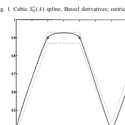
Fig. 1. CubicSG(1 ) spline, Bessel derivatives; restrictions violated.
Fig. 2. Range restrictedSG(1 ) spline, Bessel derivatives.
Remark 10. Applying the rational quintic splines (22), or the rational cubic splines (28), (29), the described method of range restricted C1 interpolation by means of tensor product methods can be immediately extended to interpolation of C2 continuity.
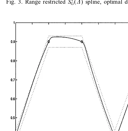
Fig. 3. Range restrictedSG(1 ) spline, optimal derivatives.
Fig. 4. Range restrictedS1
2(1) spline, optimal derivatives.
4. Numerical demonstrations
Fig. 5. Data points.
Fig. 6. Range restricted spline from S21(
x
1)⊗S21(
y
1), optimal derivatives.
weakly satised, i.e., if the upper and lower bounds are nearby equal in some nodes. In view of the formulae (16), (17) and (52), (54)–(56), corresponding tension parameters then are very large. In our examples we have chosen the compatibility conditions to be well satised.
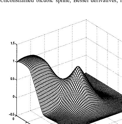
Fig. 7. Unconstrained bicubic spline, Bessel derivatives; restrictions violated.
Fig. 8. Range restricted spline fromSG(1 x)⊗SG(1 y), Bessel derivatives.
If we use the Bessel derivatives (19) we get the spline plotted in Fig. 1; the obstacles are not met in all subintervals. If the tension parameters i are determined by (16), (17), the range is restricted
as desired; see Fig. 2. Next, the derivative parameters are computed by optimizing the Holladay functional (21) using the above tension parameters; the result is the spline shown in Fig. 3. For comparison, we have also plotted the interpolant from the spline classS1
on rened grids 1; see Fig. 4. The used formula for placing the additional nodes (×) can be found in the papers [13, 17]. Again, the spline is optimal with respect to the Holladay functional. In our example, the spline from S1
2(1) (Fig. 4) does not compete with the ones from the present class
S1
G() of Gregory’s splines (Figs. 2 and 3). The same relation is observed for the tensor product
interpolants presented in the Figs. 6–8. The used data set (xi; yj; zi; j), i; j= 0; : : : ;4 is visualized in
Fig. 5, and the continuous piecewise bilinear bounds L and U are prescribed by
Li; j=zi; j−0:15; Ui; j=zi; j+ 0:15; i; j= 0; : : : ;4:
We refer to [13] for details of computing the spline interpolants from S1
2(x1)⊗S21(
y
1) on rened rectangular grids.
Acknowledgements
Both authors are supported by the Deutsche Forschungsgemeinschaft under grant Schw 469/3-1. We also wish to thank the referee for valuable comments and suggestions.
References
[1] L.-E. Andersson, T. Elfving, Best constrained approximation in Hilbert space and interpolation by cubic splines subject to obstacles, SIAM J. Sci. Comput. 16 (1995) 1209 –1232.
[2] M. Bastian-Walther, J.W. Schmidt, Gregory’s rational cubic splines in interpolation subject to derivative obstacles, in: M.D. Buhmann, M. Felten, D.H. Mache (Eds.), Second Internat. Dortmund Meeting on Approx. Theory 98, to appear.
[3] R. Delbourgo, J.A. Gregory, Shape preserving piecewise rational interpolation, SIAM J. Sci. Statist. Comput. 6 (1985) 967–976.
[4] A.L. Dontchev, Best interpolation in a strip, J. Approx. Theory 73 (1993) 334 – 342.
[5] T. Elfving, L.-E. Andersson, An algorithm for computing constrained smoothing spline functions, Numer. Math. 52 (1988) 583 –595.
[6] T.N.T. Goodman, B.H. Ong, K. Unsworth, Constrained interpolation using rational cubic splines, in: G. Farin (Ed.), NURBS for Curve and Surface Design, SIAM, Philadelphia, PA, 1991, pp. 59 –74.
[7] J.A. Gregory, Shape preserving spline interpolation, Computer-Aided Design 18 (1986) 53 – 57.
[8] M. Herrmann, B. Mulansky, J.W. Schmidt, Scattered data interpolation subject to piecewise quadratic range restrictions, J. Comput. Appl. Math. 73 (1996) 209 –223.
[9] W. He, J.W. Schmidt, Direct methods for constructing positive spline interpolants, in: P.J. Laurent, A. Le Mehaute, L.L. Schumaker (Eds.), Wavelets, Images and Surface Fitting, Chamonix 1993, A.K. Peters, Wellesley, 1994, pp. 287–294.
[10] B. Mulansky, Tensor products of convex cones, in: G. Nurnberger, J.W. Schmidt, G. Walz (Eds.), Multivariate Approximation and Splines, Internat. Ser. Numer. Math., vol. 125, Birkhauser, Basel, 1997, pp. 167–176.
[11] B. Mulansky, J.W. Schmidt, Nonnegative interpolation by biquadratic splines on rened rectangular grids, in: P.J. Laurent, A. Le Mehaute, L.L. Schumaker (Eds.), Wavelets, Images and Surface Fitting, Chamonix 1993, A.K. Peters, Wellesley, 1994, pp. 379 –386.
[12] B. Mulansky, J.W. Schmidt, Powell–Sabin splines in range restricted interpolation of scattered data, Computing 53 (1994) 137–154.
[13] B. Mulansky, J.W. Schmidt, M. Walther, Tensor product spline interpolation subject to piecewise bilinear lower and upper bounds, in: J. Hoschek P. Kaklis (Eds.), Advanced Course on Fairshape, Teubner, Stuttgart, 1996, pp. 201–216.
[15] B.H. Ong, K. Unsworth, On non-parametric constrained interpolation, in: T. Lyche, L.L. Schumaker (Eds.), Mathematical Methods in Computer Aided Geometric Design II, Academic Press, New York, 1992, pp. 419 – 430. [16] J.W. Schmidt, W. He, Spline interpolation under two-sided restrictions on the derivatives, Z. Angew. Math. Mech.
69 (1989) 353 – 365.
[17] J.W. Schmidt, W. He, Numerical methods in strip interpolations applyingC1,C2, andC3 splines on rened grids, Mitt. Math. Ges. Hamburg 16 (1997) 107–135.
[18] J.W. Schmidt, M. Walther, Gridded data interpolation with restrictions on the rst-order derivatives, in: G. Nurnberger, J.W. Schmidt, G. Walz (Eds.), Multivariate Approximation and Splines, Internat. Ser. Numer. Math., vol. 125, Birkhauser, Basel, 1997, pp. 291–307.
[19] J.W. Schmidt, M. Walther, Tensor product splines on rened grids in S-convex interpolation, in: W. Haumann, K. Jetter, M. Reimer (Eds.), Multivariate Approximation, Math. Research, vol. 101, Akademie Verlag, Berlin, 1997, pp. 189 –202.