ANALYSIS
Green accounting and the welfare gap
Paul Turner
a, John Tschirhart
b,*
aCornerStone Energy Ad6isors,Illinois Institute of Technology,29S.LaSalle,c930,Chicago,IL60603,USA bDepartment of Economics and Finance,Uni6ersity of Wyoming,P.O.Box3985,Laramie,WY82071-3985,USA
Received 20 February 1998; received in revised form 21 December 1998; accepted 28 December 1998
Abstract
Although gross domestic product (GDP) is not intended to be a measure of societal welfare, it is often used as such. One shortcoming as a welfare measure is that it fails to account for the non-marketed value of natural resource flows. The difference between societal welfare and GDP is labelled the ‘welfare gap’. A model that accounts for both market and non-market income flows from natural capital is used to examine this gap. Societal welfare depends on private goods and the stock of natural capital. The latter is subject to a logistic growth relationship common to many non-human species. Private goods are produced using human capital and flows of natural capital. An exogenously growing human population either harvests the natural resource, produces human capital or produces the private good. Optimal control theory and dynamic simulations provide steady-state harvest and human capital growth rates which determine the steady-state natural resource stock, GDP and societal welfare growth rates. The model illustrates the feasibility of explicitly accounting for ecological relationships in economic growth models and shows that, depending on one’s preferences and the growth rate of human population and the intrinsic growth rate of natural resources, GDP may diverge substantially from the growth rate of societal welfare, leaving a large welfare gap. © 1999 Elsevier Science B.V. All rights reserved.
Keywords:Gross domestic product; Green accounting; Welfare gap
1. Introduction
Gross domestic product (GDP) measures the money value of goods and services produced in an economy during a specified time period; neither
GDP nor per-capita GDP is intended to be a measure of societal welfare. One reason why GDP is not a measure of welfare is that it does not account for the value of the natural resources upon which all production ultimately depends. The natural resource stock, often referred to as natural capital, includes soil and its vegetative cover, freshwater, breathable air, fisheries, forests,
* Corresponding author. Tel.: +1-307-766-2178; fax: + 1-307-766-5090.
waste assimilation, erosion and flood control, pro-tection from ultra-violet radiation, and so on. GDP fails to account for the non-marketed value of flows from these natural resources, including many cultural and recreational activities. Never-theless, GDP mistakenly is used often as an all-encompassing measure of societal welfare by government policy makers and private enterprise.1
Because there is a difference between societal wel-fare and GDP, which we label the ‘welwel-fare gap’, the gap is examined by introducing a model that offers a more inclusive welfare measure, one that accounts for both market and non-market income flows from natural capital.
In the model societal welfare depends on pri-vate goods and the stock of natural capital. Pri-vate goods are produced using human capital (i.e. educated workers) and flows of natural capital. The annual growth rates of per-capita income (as measured by GDP) and societal welfare are com-pared along a balanced-growth path by
employ-ing simulation modelemploy-ing software (STELLA II).2
Simulations help identify the steady-state equi-librium of the system. The objectives are to: (1) depict the feasibility of explicitly accounting for ecological relationships in economic growth mod-els; (2) illustrate the value of computer simulation exercises in extending the insights of theoretical and empirical growth models; (3) formally show that, depending on one’s preferences and the growth rate of human population and the intrin-sic growth rate of renewable resources, per-capita income growth may diverge substantially from the growth rate in per-capita welfare; and (4) use comparative statistics to examine system response to parametric changes.
This work is motivated by the debate between
mainstream economists and natural scientists3
over the importance of natural capital to human welfare. Each group contends that the other does not understand its pedagogical perspective. Hop-ing to address the most ardent concerns of each discipline, we construct a model based on the economists’ endogenous technological growth the-ory and constrained by the biologists’ logistic growth function for a renewable resource. It is assumed, as reflected in the theoretical model, that natural capital is essential to human welfare: ‘‘zero natural capital implies zero human welfare because it is not feasible to substitute, in total, purely ‘non-natural’ capital for natural capital’’ (Costanza et al. 1997).
Section 2 provides motivation for the problem, and Section 3 is a discussion of endogeneous growth theory. The difference between economic growth and economic development in the model is covered in Section 4, and the model is introduced in Section 5. Section 6 presents the model results and a conclusion follows in Section 7. Appendix A presents the model in detail.
2. Motivation
Disciplinary investigation of environmental
problems by both economists and ecologists is at least two-centuries old.4There is ideologic friction
between the two groups as witnessed by the well-publicized dispute between Paul Ehrlich and the
late Julian Simon.5 This feud notwithstanding,
4The writings of classical economist Thomas Malthus fo-cused on the effect of population growth on the availability of resources necessary to sustain human existence (Malthus, 1960 [1798]). Charles Darwin developed his theory of evolution around the same basic idea: species have the tendency to overproduce, with the result that only those most ‘fit’ to their environmental circumstances survive and reproduce (Darwin, 1958 [1859]).
5The well-publicized wagers between Ehrlich (1981, 1982) and Simon (1981b) on the direction of future welfare measures highlight the philosophical rift between ecologists and main-stream economists (Shen, 1996). Simon’s exuberance to bet on ‘‘...anything pertaining to material human welfare...’’ refers almost exclusively to income-based welfare indices neglecting the value of the natural capital on which all economic output is ultimately based (Shen, 1996).
1For example: ‘‘Today the two political parties differ some-what in regard to means, but neither disputes that the ultimate goal of national policy is to make the big gauge — the gross domestic product — climb steadily upward.’’ (Cobb et al., 1995)
2STELLA II is a simulation modeling software package used to model complex systems including ecosystems and economic systems. See Hannon and Ruth (1994).
interdisciplinary research between ecologists and economists will play an important role in address-ing social problems concurrent with an increasaddress-ing human population whose consumption hastens the rate of ecosystem degradation.
Mainstream neoclassical economists, slow to appreciate the importance of maintaining a healthy and productive environmental resource base, are beginning to accept ecologists’ asser-tions. Nobel laureate economists Robert Solow and Kenneth Arrow recognize the inextricable link between biological and economic systems, and urge a more careful consideration of account-ing for biological degradation in economic growth statistics (Solow, 1994; Arrow et al., 1995). While difficult, fraught with uncertainties, and opposed by many as immoral, valuing ecosystems is neces-sary when making choices. Ecologists, economists and geographers have estimated the value of na-ture’s long list of ecosystem goods and services6
and argue that such an exercise is important in order to ‘‘make the range of potential values of
the services of ecosystems more apparent’’
(Costanza et al., 1997).
While some economists are heeding the biologi-cal wake-up biologi-call, others, such as Simon (1981a, 1995a), continue to downplay the economic and sociological importance of maintaining a healthy and viable natural resource base. According to Simon, society’s ability to advance technology as necessary should obviate concern for the genius to concoct, devise, and invent ways around barriers that threaten production (and consumption). Be-cause humans have acquired the technology for nuclear fission and space travel, they now have all the tools necessary to
‘‘…go on increasing our population forever, while improving our standard of living and
control over our environment’’. (Simon, 1995b)
Simon’s forecasts are optimistic: the environ-mental degradation associated with continued population growth and increasing per-capita con-sumption will test society’s collective intellect.7
Presuming that past trends of technological pro-gress can be relied on to overcome the
environ-mental stresses concurrent with growing
populations is a risky strategy. Humankind cur-rently appropriates approximately 40% of total net terrestrial primary production of the bio-sphere (Vitousek et al., 1986), 25 – 35% of coastal shelf primary production (Pauly and Christensen, 1995), and half of the available global supply of fresh water (Postel et al., 1996). There is ample
evidence that the carrying capacity8 of many
ecosystems is being severely tested (Kirchner et al., 1985; Rees, 1990; Hardin, 1991; Brown, 1994, 1995). Mapping a course through this uncharted ecological territory should not be left solely to unfettered markets.9
Because more people means more land devoted to human habitat and less land devoted to habitat for the millions of other species, Simon’s forecasts also downplay the amenity value of nature. Peo-ple place positive value on many environmental amenities (and negative value on disamenities) which are not easily traded in markets. The tricky part is placing an actual dollar value on these amenities. Economists interested in quantifying use and non-use values for nature’s goods employ a variety of measurement techniques such as travel-cost method, hedonics and contingent valu-ation method. The validity and applicability of
7The precipitation of violent civil or international conflict caused by renewable resource scarcity is another concern for researchers of environmental issues (Homer-Dixon, 1994).
8Carrying capacity is often defined as ‘‘the maximum popu-lation of a given species that can be supported indefinitely in a defined habitat without permanently impairing the productiv-ity of that habitat’’ (Rees, 1994).
9The history of Easter Island provides a good example of the catastrophic social effects of exhausting a renewable re-source when the availability of adequate substitutes is severely restricted (Ponting, 1991).
the economic values obtained using these valua-tion techniques are sometimes suspect but the premise holds: people value environmental re-sources, especially when few satisfactory substi-tutes exist.
3. Endogenous growth theory and population
Starting with the seminal work of Solow (1957), substantial economics literature, catalogued under the title of ‘‘endogenous technological-growth the-ory’’, has sought to explain economic growth.10
In these models, physical (or human-made) capital, human capital (education) and the latest produc-tion technology are combined to generate output which can be re-invested in human-capital (saved) or consumed. While conventional endogenous growth models track investment in physical and human capital stock, few models explicitly incor-porate the biological growth/stock relationship of a renewable resource:11 the supply of natural
re-sources is considered limitless. This assumption is challenged and the role of natural capital in the production process elevated while discounting the explicit importance of human-made capital.12
Re-quiring the production process to adhere to the behavior of a natural system such as the fishery or forest subjects the economy to a biological constraint.
Essentially all endogenous growth models of knowledge predict that technological progress is an increasing function of population size. (Romer, 1996). The larger the population, the more people there are to make discoveries and, thus, the more
rapidly knowledge accumulates. Alternative inter-pretations hold that over almost all of human history, technological progress has led mainly to increases in population rather than increases in output per person (Kremer, 1993).13
Neglected in these stories is the impact of grow-ing populations on natural resource stocks. More efficient harvesting of natural capital along with a growing human population has had a substantial effect on reducing the resource stock of the world’s major fisheries and rainforests (Dietz and Rosa, 1994; Brown, 1995; Resources, 1996). Economists who believe population growth is conducive to economic growth cite data showing that in most parts of the world, food production and per-capita gross income have generally grown since the end of World War II (Dasgupta, 1995a). These figures ignore the depletion of the natural resource base.
4. Economic growth versus economic development
‘‘The general proposition that economic growth is good for the environment has been justified by the claim that there exists an empir-ical relationship between per-capita income and some measures of environmental quality. …as income goes up there is increasing environmen-tal degradation up to a point, after which envi-ronmental quality improves (The relation has an ‘inverted-U’ shape)… in the earlier stages of economic development, increased pollution is regarded as an acceptable side effect of eco-nomic growth. However, when a country has attained a sufficiently high standard of living, people give greater attention to environmental amenities.’’ (Arrow et al., 1995)
The inverted U-shaped curve has been shown to apply to a select set of pollutants (as quoted in Arrow et al. (1995)). Some economists have
sug-10Other than Arrow’s ‘learning-by-doing’ paper from 1962 (Arrow, 1962), economic growth theory garnered little atten-tion until rejuvenated by work by Lucas (1988), Stokey (1988), Barro (1991) and Romer (1986, 1987). Sparked by the seminal work by Barro (1991), there has been an explosion in empirical work on economic growth by authors such as Jones (1995), Sala-i-Martin (1996, 1997) and Sachs and Warner (1997).
11This quadratic relationship between a biological stock and its instantaneous growth rate is often represented with the Schaefer curve (Gordon, 1954; Schaefer, 1957; Clark, 1990).
12Daly (1991), Daly and Cobb (1994), Arrow et al. (1995), and Dasgupta (1995b).
gested that the notion of people spending propor-tionately more of rising incomes on environmen-tal quality also applies to the natural resource base. While economic growth is associated with improvements in some environmental indicators, it is not a sufficient condition for general environ-mental improvements nor is it a sufficient condi-tion for the earth supporting indefinite economic growth. In fact, if this base were severely de-graded, economic growth itself could be jeopar-dized (Arrow et al., 1995).
Although GDP is commonly used as a measure of economic health and even personal well being, it is far from adequate as a measure of true
economic performance.14Numerous authors point
out the need for a more comprehensive index that includes the flow of environmental services as well as the value of net changes in the stocks of natural capital so that the true social costs of growth are internalized. A better indicator would ameliorate the conflict between growth and the environment by subtracting environmental deple-tion from the index. The United Nadeple-tions has recommended accounting for depletion in ‘satel-lite accounts’ as opposed to including depletion in the main tables. Repetto et al. (1989) have argued forcefully against this approach as it continues the use of misleading economic indicators, and these same authors have offered methodologies to im-prove national accounting.
Net domestic product (NDP), calculated by deducting environmental degradation of the re-source base from GDP, is a more inclusive mea-sure of personal well-being today and tomorrow
(as quoted by Dasgupta (1995b)).15 That NDP is
a better measure of the improvement in societal well-being is similar to the claim of Daly and Cobb (1994) that economic development is a bet-ter measure of well being than economic growth. (These authors also highlight the importance of sustainability, but sustainable issues are not di-rectly addressed in this paper.16 Repetto et al.
(1989) indicate that only by including environ-mental depletion into the national accounts will ‘‘…economic policy be influenced toward sustain-ability’’. (p.12)) The analysis is concerned with an optimal growth path that includes the unhar-vested natural resource stocks in the welfare func-tion, and it is, therefore, consistent with using some form of NDP.
The model herein allows the social planner to make perfectly timed, precise adjustments to the harvest and human capital investment rates that keep the bionomic system at, or returns it to, a
steady-state equilibrium along the balanced
growth path. Assuming the social planner has perfect information in such decisions is unrealis-tic. As pointed out by Stiglitz (1996), informa-tional uncertainty pervades economies making identification of and adherence to a balanced growth path and overly optimistic outcome. In-cluding a time lag to represent the reaction and adjustment process associated with data accumu-lation and analysis, or an uncertainty parameter to represent the inherent lack of analytical preci-sion would add realism to the model. Either mod-ification would almost certainly provide results different from those presented here. Time lags and uncertainty may prevent adherence to the bal-anced growth path and possibly even preclude maintenance of a steady-state equilibrium. If suffi-ciently severe, the bionomic system could tend toward a socially undesirably corner solution with complete exhaustion of the natural resource. Ex-ploration of these issues is left for further research.
14The Bush Administration acknowledged this in the Coun-cil on Environmental Quality Annual Report (1992). ‘‘Ac-counting systems used to estimate GDP do not reflect depletion or degradation of the natural resources used to produce goods and services’’. Consequently, the more the nation depletes its natural resources, the more the GDP goes up.
15El Serafy (1997) also recognizes the importance of green-ing the national accounts (particularly of developgreen-ing countries) to include the flows from natural capital: ‘‘…it seems rather elementary that economists should pay attention in their anal-ysis to the sustainability of natural resources’’. (1997 p. 219)
5. Model
The social planner is responsible for maximiz-ing welfare of a representative agent from the population of identical individuals. Welfare is a function of the representative agent’s shares of the renewable natural resource stock and of the pri-vate good. The planner solves an optimal control problem with two state variables and two control variables. She chooses (i) a harvest effort rate that determines the size of the renewable natural re-source stock; (ii) the number of people devoted to human capital production (education) that deter-mines the human capital stock, and the number of people employed in private good production.
The private good, produced by combining the current production technology with human capi-tal augmented labor and natural capicapi-tal, is shared equally among the population. Preferences for natural resources and private good consumption are captured by the relative size of the coefficients in a Cobb – Douglas welfare function. Natural capital, therefore, enters the welfare function di-rectly as a stock and indidi-rectly as an input used in the production of the private good.
The model contains both rival and non-rival knowledge. The choice of how many people to devote to human capital production determines the growth rate of non-rival technology. That is, devoting a greater proportion of labor to educa-tion can increase the human capital stock. Placing labor in human capital production and applying its skills to the existing technology creates this human capital. Patenting activity is used to repre-sent the growth rate in rival knowledge. Both the human capital and private good production func-tion are generalized Cobb – Douglas funcfunc-tions. The renewable natural resource is constrained by a biologic logistic growth function. The resource might be a forest that has value left standing including both use and non-use values. The natu-ral resource is characterized as a contestable pub-lic good in that the allocation to any individual is the total stock divided by the population.
Finally, the welfare gap is used to determine how well GDP tracks societal welfare. Definingry
as economic growth measured by GDP growth
and ru as economic development measured by
welfare growth, the welfare gap isDW=ru−ry..
The optimality conditions in Appendix A provide the basis for the STELLA simulations. A comparative static analysis using STELLA is car-ried out, and the simulations show how per-capita income and welfare growth rates, the welfare gap and resource stock levels vary over time as the social planner adjusts the harvest rate and human capital investment rate in order to keep the bio-nomic system on a balanced growth path follow-ing a transient, parametric perturbation. The full model is presented in the Appendix A.
6. Results
The simulations require parameter values for
the social discount rate (r), the population
growth rate (m), and the growth rate of propri-etary technology (g). Selection of a social discount
rate is contentious (Lind, 1982): here r is the
long-run real rate of growth in GDP in the US which is about 3% (see Kahn, 1998 p. 113). Ini-tially, it is assumed that the population grows at the current average growth rate of world popula-tion (m) estimated at 1.5% (Reddy, 1996). The 3% growth rate of Fagerberg (1987) in patenting ac-tivity among OECD countries between 1974 and 1983 is used as a proxy for technological growth (g).
The importance people place on consumption relative to natural amenities and the importance of human capital relative to natural capital in the production function are captured by the coeffi-cients f and a, respectively. Initially, the relative importance of the two goods are weighted equally in the welfare function (f=0.5), as are the rela-tive importance of two inputs in the production function (a=0.5). The natural resource carrying capacity (S), is unitized which allows all steady-state harvest and resource stock values to be
expressed as a percentage of S. The intrinsic
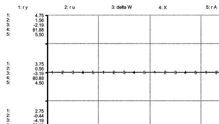
Fig. 1. Base case steady-state equilibrium.
per-capita harvest effort (6*), total harvest effort
(V*), total harvest (h*), resource stock (X*) and
human capital growth rate (rA*). The asterisk
denotes steady-state equilibrium values. The vari-ables6,V,h, and Xare measured in terms of ‘S’
and described by the ‘catch-per-unit effort hy-pothesis’ (Hartwick and Olewiler, 1986).
Modeling Appendix A Eqs. (A.11), (A.13), (A.14), (A.16), (A.17), (A.18) and (A.19) in STELLA allows investigation of the behavior of the rates of human capital growth, economic growth, economic development and the welfare gap along the balanced growth path in both steady-state and transient periods. Fig. 1, which is generated by STELLA, establishes the base case scenario where the system is initially in a steady-state equilibrium. Curves 1, 2, 3, 4 and 5 in Fig. 1 show that if the initial resource stock equals the steady-state stock, economic growth or GDP (ry), economic development (ru), the welfare gap (DW),
the natural resource stock (X) and the human
capital growth rate (rA) start and remain at their steady-state levels. The resource stock initially starts at its steady-state level, X* and the social planner makes the requisite adjustments to keep
the bionomic system in a steady-state equilibrium along the balanced growth path. To obtain Fig. 1, the social planner maximizes intertemporal wel-fare by choosing optimal steady-state harvest rates and human capital accumulation rates that
result in an optimal steady-state stock of
80.875%17and a human capital accumulation rate
of 4.50%. Consequently, per-capita GDP in-creases at an annual rate of 3.75% with per-capita welfare growing at 0.5625% annually. A negative
welfare gap (DW*= −3.1875%) implies that
given the model’s parameters, per-capita GDP overstates the rate at which people’s lot in life is improving by 3.1875%.
Simulations identify the steady-state
equi-librium, and they are also helpful in examining how parametric changes from the status quo af-fect the transient and steady-state behavior of the system. Consider two cases in which: (1) prefer-ences for preserving the natural resource stock
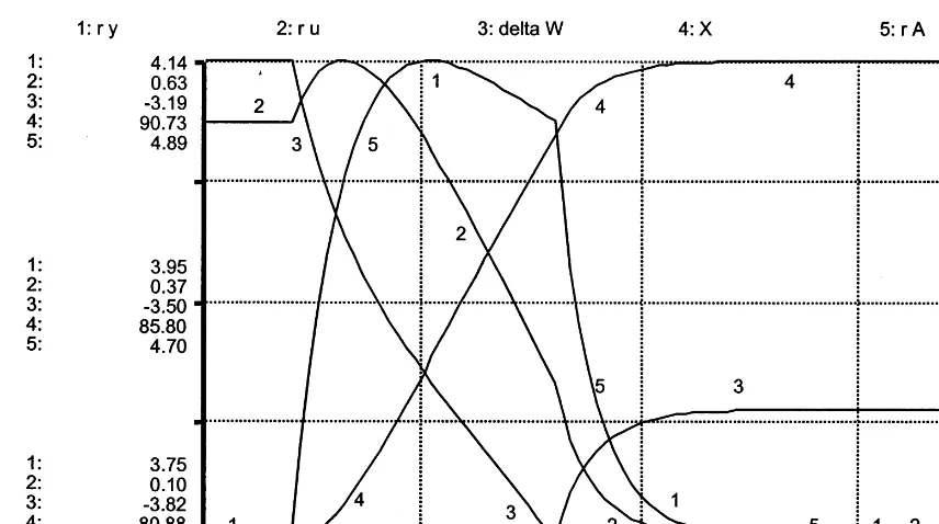
Fig. 2. Effect of step-change in preference for natural resource (f) att=10.
and (2) population growth change over a discrete time period. In the first case, the relative weight placed on the private good in the welfare function (1−f) is decreased while the weight placed on the natural resource stock (f) is increased. Spe-cifically, f is increased at an annual rate of 1% over the time period t=10 – 40. The increasing weight on the natural resource stock reflects the ‘inverted-U’ hypothesis discussed above which maintains that as a society enjoys economic pros-perity, it will place more emphasis on the environ-ment. In the second case, the current population growth rate (m) is increased at an annual rate of 1% over the time periodt=10 – 40, after which it remains at its new level for the remaining analysis period.
Fig. 2 pertains to case (1). The system is ini-tially at the steady-state equilibrium shown in Fig. 1. At t=10, the preference for natural resources begins to increase at an annual rate of 1%. As expected, the natural resource stock begins to climb owing to lower harvests. To compensate for the lower harvest rate, the social planner increases the rate of human capital accumulation (rArises). This trend continues until the point where, given
the decreased flow from the natural capital stock, the marginal returns from additional human capi-tal investment begin to decline at approximately
t=25 (ryfalls). At this point, lower harvest levels
encourage a decrease in the human capital invest-ment rate. At t=40, the preference for natural resources stops increasing and holds steady at
approximately f=0.67. The resource stock
in-creases to a new steady-state level of 90.73% with the human capital growth rate eventually return-ing to its initial steady-state level of 4.5%.
During this time when the preference for natu-ral resources is increasing, the social planner
ad-justs the harvest rate and human capital
accumulation rate to remain on the balanced-growth path. In turn, this adjustment process affects GDP and welfare growth rates (ryandru).
Initially in a steady-state equilibrium, GDP growth rate begins to climb in conjunction with the rise in the human capital growth rate.18
How-ever, as the growth rate in human capital falls, the GDP growth rate eventually returns to its pre-per-turbation steady-state level.19
The transient and
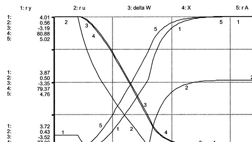
Fig. 3. Effect of step-change increase in population growth rate (m) att=10.
post-perturbation behavior of the growth rate in welfare differs significantly from the growth rate in GDP. Initially in steady-state at approximately 0.56%, the welfare growth rate first climbs in response to the increase in the resource stock and
GDP growth rate20reaching a maximum of about
0.63%. As the rate of increase in GDP growth rate begins to diminish, the welfare growth rate begins to fall in conjunction with the increase in prefer-ences for the natural resource. This is attributable to natural resource preferences increasing faster than the stock of natural resources, so that even though the resource stock and its relative weight in the welfare function is increasing, the net effect cannot overcome an increasing GDP growth rate whose relative weight is declining. As seen in Eq. (A.14), because the steady-state GDP growth rate returns to its pre-perturbation level but is now weighted less in the welfare function, the new steady-state value for the welfare growth rate is less than its pre-perturbation level. Thus, even though the natural resource stock and its relative weight in the welfare function are larger, the net
effect is a lower steady-state welfare growth rate. The welfare gap, as measured by DW, initially at
−3.1875%, continues to widen as the preference
for natural resources increases. When the welfare weight placed on natural resources reaches a new steady-state at 0.675 at t=40, the widening trend ceases and the steady-state welfare gap increases slightly to −3.65%. The new steady-state welfare gap is wider than its pre-perturbation level. These changes capture the notion that as preference for the natural resource increases relative to GDP, the welfare gap widens.
In Fig. 3, system sensitivity is examined to an annual 1% increase in the population growth rate from its original steady-state value of 1.5% at
t=10 to a new-steady-state value of 2.02% at
t=40. When the population growth rate begins to increase, the added population results in an in-crease in the number of people involved in human capital production, private good production and resource harvesting. The increase in the steady-state human capital growth rate from 4.50 to 5.02% is wholly a result of the increased popula-tion growth rate with none of the increase due to a change in the percentage of labor working in
private good production and that devoted to hu-man capital production.21
Even after the popula-tion growth rate levels off at 2.02% att=40, the human capital growth rate does not reach its new steady-state equilibrium until t=70. It takes the system time to accommodate the changes insti-gated by the parameter change.
The natural resource stock sees its steady-state stock decline from 80.875 to 77.857%. Reflective of the increased demand for private good concur-rent with a larger population, total output in-creases as the increased human capital stock requires additional natural resources. The added population each period results in an increase in total consumption, which requires an increase in the steady-state harvest rate and a decline in the natural resource stock to a lower steady-state equilibrium.22
The decline in resource stock that begins at
t=10 results in the income growth rate initially declining until the human capital growth rate increases to compensate. The rapid accumulation of human capital stock leads to an increase in the
income growth rate until t=40. As the
popula-tion growth rate stabilizes at 2.02%, the income growth rate continues to increase but at a decreas-ing rate. In a sense, the social planner, recognizdecreas-ing that the perturbation has ended, is no longer required to take the drastic steps necessary to keep the system on the balanced growth path. The new steady-state per-capita income growth rate is now at a higher level as a result of the higher steady-state population growth rate.23
As a result of the initial decline in both the resource stock and income growth rate, and the need to now share the stock and income with more people, the welfare growth rate witnesses a precipitous decline at t=10. Even after the in-come growth rate recovers and begins to increase,
the protracted decline in the per-capita share of resource stock results in a continued decline in welfare growth reaching a low point of 0.428% at
t=40. Heretofore, the stock, declining at an in-creasing rate, continues to decline after t=40 but
at a decreasing rate.24 The net result of this
change is a partial recovery for the welfare growth rate from its minimum of 0.428% to a new steady-state equilibrium of 0.497%. The new steady-steady-state welfare growth rate of 0.497% is lower than its pre-perturbation level of 0.5625%.
The gap between the growth rates in GDP and welfare widens as the growth rate in population increases. That is, the faster population multiplies, the greater the divergence between per-capita GDP and welfare growth rates. The reason for this divergence is primarily the reduced natural resource stock. As mentioned before, the stock declines from 80.875 to 77.857% while concur-rently the number of people who share it in-creases. The net effect is less public good per-capita, which leads to a decline in the welfare growth rate and an increase in the welfare gap.
7. Conclusion
Standard methods employed to solve dynamic problems such as those seen in the endogenous growth literature are often unable to accommo-date modifications such as the parabolic behavior of renewable resources. The clever method of Romer (1990) of identifying the balanced growth path was not, by itself, sufficient to solve our problem of accounting for the behavior of a non-linear, biological growth function. The simulation software allowed the retention of the most inter-esting characteristics of the problem while also providing a tractable solution. It is felt that simu-lations can also be employed to provide insights and possibly help solve problems that heretofore have been beyond the scope of traditional solu-tion methods.
Using simulations, the growth rate expressions for GDP and welfare are used to examine why a
21This can be seen by comparing the percentage changes betweenmandrA.
22This is different from the situation depicted in Fig. 2 where the increase infeventually led to diminishing returns to additional human capital investment which resulted inry returning to its original steady-state level.
commonly used indicator such as per-capita GDP is a poor proxy for per-capita welfare owing to the welfare gap. In steady-state, the per-capita income growth rate exceeds the per-capita welfare growth rate.
Simulations generated with STELLA were em-ployed to examine how the variables in the model are affected by a slight but persistent parametric perturbation. This exercise helps to illustrate how the social planner adjusts the harvest rate and human capital accumulation rate in response to the parametric perturbation. The parameter that changes influences the size of DW*. However, as shown above, the effect onryandruis not always permanent, illustrating that some exogenous parameter shifts cause only transient changes. Once the perturbation ceases, the income or wel-fare growth rate may return to its original steady-state levels.
These results have important policy implica-tions. For example, a policy that encourages higher population growth does increase per-capita income; however, the policy also diminishes wel-fare growth resulting in an increase in the welwel-fare gap. As expected, a policy designed to improve technology will have the intended effect of nar-rowing the welfare gap. And policymakers in developing countries may question the ‘inverted-U’ relationship between income growth and envi-ronmental quality; while an increase in preference for the natural resource does increase the natural resource stock, it leads to a decline in the steady-state welfare rate.
Growth theoretic models are highly abstract, extremely aggregated representations of the real world. Nevertheless, empirical applications of growth models are used by economists in attempts to explain the wide divergences in living standards across nations, and why some countries seem to be making the transition from less to more devel-oped, while other countries remain in poverty. Absent from these models is any recognition that economies function in and depend on a biological world that places limits on physical growth. When Solow first introduced his growth model in the 1950s, these biological constraints may have seemed more remote because the world’s popula-tion was half of what it is today. The results
suggest that models which continue to ignore the biological constraints are desperately incomplete; they will yield misleading guidance owing to their focus on income growth instead of a more com-plete welfare measure.
Appendix A
The per-capita growth expressions for income and welfare are derived from a one-region en-dogenous technological growth model that is con-strained by a natural capital production function. Welfare for a representative individual is based on her consumption of a public and private good. All people in the region (m+n) share a private good,
Y, produced using the harvested renewable
re-source. The individual also derives welfare from that portion of renewable resource that remains
unharvested, X. The renewable resource
repre-sents a public good such as a forest or fishery and is shared among everyone in the region (m+n).
In the instantaneous welfare function, (A.1), h
determines the consumer’s attitude toward
in-tertemporal consumption. The smaller is h, the
more slowly marginal welfare falls with a rise in
consumption. It is assumed that h=0.5 in the
model. The relative weight that one places on the unharvested resource stock (private good) is rep-resented by f (1−f).
The goal is to maximize intertemporal welfare by identifying the optimal per-capita consumption path for the resource and private good. Welfare is constrained by a biological growth function and human capital stock accumulation relationship.
Y=(A(n−HA))a(6
mX)1−a(
G)a−1
and A(0)=A0 6mX(0)=(6mX)0
The relative importance of the productive in-puts is captured in the Cobb – Douglas production coefficient (a). The larger isa, the more important is labor in the production process and the less important is natural capital. The subjective dis-count weight on consumption isr. The constraint on the renewable resource stock is represented by the biological growth relationshipF(X)=gX(1−
X/S) where g depicts the intrinsic biological
growth rate and S the carrying capacity of the
resource (Hartwick and Olewiler, 1986). The hu-man capital constraint,A: , is a function of
educa-tional success, s, the current stock of human
capital,A, and the number of people involved in human capital production, HA.
A frequently used assumption in endogenous growth models is to have population growing at a constant rate (Romer, 1996). All population terms are assumed to grow at the constant ratem(m=
memt, n=n emt, m+n=(m+n) emt, and HA=
HAemt). Also, proprietary production technology
that converts natural capital to a durable good of any design grows at a constant rate,g(G=Gegt),
whereGrepresents the current state of technology by denoting the amount of natural capital neces-sary to produce one unit of private good. Because the exponent on Gin the production function for
Y is negative, g must be negative in order to
represent improving production technology with large negative values representing relatively better technology. An increase in g represents a reduc-tion in (or worsening of) the growth rate of production technology; it takes more natural cap-ital to produce one unit of private good. Making these substitutions, m, n, HA, and G represent initial condition levels and the problem becomes
Maximize
The current-value Hamiltonian can be ex-pressed as:
There are four first-order conditions: one for the control variable,6, ((Hc/(6)=0, and its
corre-for the control variable 6 in terms of l
X, the
shadow price of the resource, gives
lX=
The first-order condition for Xis
l:X= −
Dividing (A.4) by (A.3) provides
l:X lX
=C−F%− f
(1−a)(1−f)6me
mt (A.5)
Solving the first-order condition for the control variable HA in terms of lA, the shadow price of
human capital investment, provides
lA=
l:A=
Dividing (A.7) by (A.6) gives
l:A
Solving the system explicitly for its dynamics is complex. To simplify the analysis, the discussion is focused on the properties of the balanced growth equilibrium inherent in the model. Eq. (A.9) illustrates a basic feature of the steady-state equilibrium: along the balanced growth path, the growth rate of the human capital stock (rA=A: /
A) equals the sum of the growth rates of natural capital, population and proprietary production technology.
rA=X:
X+m+g (A.9)
As Romer shows in his paper (1990), in steady-state, l:A/lA=l:X/lX. Equating (A.5) and (A.8)
and using (A.9) provides the steady-state expres-sions for the optimal harvest effort level (V) and the optimal human capital growth rate (rA) as a function of the various system parameters, Cobb – Douglas production and welfare coefficients and resource stock level (see A.10 and A.12).
With the resource stock variableXstill present, Eq. (A.10) and Eq. (A.11) do not accurately rep-resent the first-order conditions for V and HA.
The expression for the biological growth function
could be used to eliminate X from (A.10) and
(A.11). However, solving this quadratic equation for X requires assumptions that detract from the issues of interest.25 For this reason, dynamic
sim-ulations are used to determine the optimal steady-state equilibrium for the bionomic system.
The expressions for per-capita income and wel-fare growth rates are obtained from (A.1). In Eq. (A.12),y represents the equal income share to all agents in the region.
y= Y
m+n=
(A(n−HA)a(6mX)1−a
Ga−1)
m+n (A.12)
Totally differentiating (A.12) with respect to time, (A.13) represents the general expression for the growth rate in per-capita income along the balanced growth path
ry;
y=arA+(1−a)
X:
X+g
n
(A.13)with the steady-state growth rate of per-capita income represented by (A.14)
r*y=am+g (A.14)
where the ‘*’ represents a steady-state equilibrium value.26
Knowing that per-capita welfare is represented by
25For example, assuming that is valid for steady-state con-ditions but not accurate for transient periods when X is changing.
u= 1
the growth rate expression for per-capita welfare is
ru=(1−h)
8X:
X−m
+(1−f)ryn
(A.16)In steady-state, (A.16) becomes
ru*=(1−h)[(1−f)ry*−8m] (A.17)
The difference between ru and ry is the welfare gap,DW(DW=ru−ry). Using (A.13) and (A.16), the general welfare gap along a balanced growth path can be written as
DW=f
X:X−rA−am
n
(A.18)with (A.19) representing the welfare gap in steady-state.
DW *= −f[rA*+am] (A.19)
References
Arrow, K., 1962. The Economic Implications of Learning by Doing. Review of Economic Studies. 29, 155 – 173. Arrow, K., Bolin, B., Costanza, R., Dasgupta, P., Folke, C.,
Holling, C.S., Jansson, B., Levin, S., Ma¨ler, K., Perrings, C., Pimentel, D., 1995. Economic growth, carrying capac-ity, and the environment. Science 268, 520 – 521.
Barro, R., 1991. Economic growth in a cross section of countries. Quart. J. Econ. 106, 407 – 443.
Brown, L., 1994. State of the World. W.W. Norton, New York.
Brown, L., 1995. State of the World. W.W. Norton, New York.
Clark, C., 1990. Mathematical Bioeconomics: The Optimal Management of Renewable Resources, 2nd edition. Wiley, New York.
Cobb, C., Halstead, T., Rowe, J., 1995. If the GDP is up, why is America down? Atlantic Monthly 276(4) 59 – 78. Costanza, R., d’Arge, R., de Groot, R., Farber, S., Grasso,
M., Hannon, B., Limburg, K., Naeem, S., O’Neill, R., Paruelo, J., Raskin, R., Sutton, P., van den Belt, M. 1997. The Value of the World’s Ecosystem Services and Natural Capital. Nature 387, 253 – 260.
Council on Environmental Quality Annual Report, 1992. Ex-ecutive Office of the President, Council on Environmental Quality. Washington D.C.
Daly, H., 1991. Steady-State Economics: Second Edition with New Essays. Island Press, Washington DC.
Daly, H., Cobb, J., 1994. For the Common Good. Beacon Press, Boston.
Darwin, C., 1958 [1959]. The Origin of Species. New American Library, New York.
Dasgupta, P.S., 1995a. Population, poverty and the local environment. Sci. Am. 272(2), 40 – 45.
Dasgupta, P.S., 1995b. The population problem: theory and evidence. J. Econ. Lit. 33, 1879 – 1902.
Dietz, T. and Rosa, E.A., 1994. Rethinking the environmental impacts of population, affluence and technology. Hum. Ecol. Rev. 1.
Ehrlich, P.R., 1981. An economist in wonderland. Social Sci. Quart. 62, 44 – 49.
Ehrlich, P.R., 1982. That’s right you should check it for yourself. Social Sci. Quart. 63, 385 – 387.
El Serafy, S., 1997. Green accounting and economic policy. Ecol. Econ. 21, 217 – 229.
Fagerberg, J., 1987. A technology gap approach to why growth rates differ. Res. Policy 16, 87 – 99.
Gordon, H., 1954. Economic theory of a common-property resource: the fishery. J. Polit. Econ. 62, 124 – 142. Hannon, B., Ruth, M., 1994. Dynamic Modeling.
Springer-Verlag, New York.
Hardin, G., 1991. Paramount positions in ecological econom-ics. In: Costanza, Robert (Ed.), Ecological Economics: The Science and Management of Sustainability. Columbia Uni-versity Press, New York.
Hartwick, J., Olewiler, N., 1986. The Economics of Natural Resource Use. Harper-Collins, New York.
Homer-Dixon, T., 1994. Environmental scarcities and violent conflict: evidence from cases. Int. Security 19, 5 – 40. Jones, C., 1995. Time series tests of endogenous growth
mod-els. Quart. J. Econ. 110, 495 – 525.
Kahn, J., 1998. The Economic Approach to Environmental and Natural Resources. The Dryden Press, Fort Worth, TX.
Kremer, M., 1993. Population growth and technological change: one million B.C. to 1990. Quart. J. Econ. 108, 681 – 716.
Kirchner, J., Leduc, G., Goodland, R., Drake, J., 1985. Carry-ing capacity, population growth, and sustainable develop-ment. In: Mahar, D. (Ed.), Rapid Population Growth and Human Carrying Capacity: Two Perspectives. The World Bank Staff Working Papersc690, Population and Devel-opment Series, Washington DC.
Lind, R., 1982. Discounting for Time and Risk in Energy Policy. Resources for the Future, Washington DC. Lucas, R., 1988. On the mechanics of economic development.
J. Monetary Econ. 22, 3 – 42.
Pauly, D., Christensen, V., 1995. Primary production required to sustain global fisheries. Nature 374, 255 – 275. Ponting, C., 1991. A Green History of the World. Penguin
Books, New York.
Postel, S.L., Daily, G.C., Ehrlich, P.R., 1996. Human appro-priation of renewable fresh water. Science 271, 785 – 788. Reddy, M., 1996. Statistical Abstract of the World, 2nd
edi-tion. Gale Research, Detroit.
Rees, W., 1990. Sustainable development and the biosphere. Ecologist 20, 18 – 23.
Rees, W., 1994. Presented at the International Workshop on Evaluation Criteria for a Sustainable Economy. Institute fur Verfahrenstechnik. Technische Universitat Graz, Graz, Austria.
Repetto, R., Magrath, W., Wells, M., Beer, C., Rossini, F., 1989. Wasting Assets: Natural Resources in the National Income Accounts. World Resources Institute, Washington, DC.
Resources, 1996. Resources for the Future, Washington DC. Romer, P., 1986. Increasing returns and long-run growth. J.
Polit. Econ. 94, 1002 – 1037.
Romer, P., 1987. Crazy Expectations for the Productivity Slowdown. NBER Macroeconomics Annual. MIT Press, Cambridge.
Romer, P., 1990. Endogenous technological change. J. Polit. Econ. 98, S71 – S102.
Romer, D., 1996. Advanced Macroeconomics. McGraw-Hill, New York.
Sachs, J., Warner, A., 1997. Fundamental Source of Long-Run Growth. American Economic Review, Papers and Proceedings.
Sala-i-Martin, X., 1996. The classical approach to convergence analysis. Econ. J. 106, 1019 – 1036.
Sala-i-Martin, X., 1997. I just ran two million regressions. Am. Econ. Rev. 87, 178 – 183.
Schaefer, M., 1957. A study of the dynamics of the fishery for yellowfin tuna in the eastern tropical Pacific Ocean. Bull. Inter-Am. Trop. Tuna Commission 2, 247 – 285.
Shen, F., 1996. Professor’s $100 000 Slice of Pie in the Sky. The Washington Post, Washington, DC (February 6). Simon, J., 1981a. The Ultimate Resource. Princeton
Univer-sity Press, Princeton.
Simon, J., 1981b. Paul Ehrlich saying it is so doesn’t make it so. Social Sci. Quart. 63, 181 – 185.
Simon, J., 1995a. The Ultimate Resource II. Princeton Univer-sity Press, Princeton.
Simon, J., 1995b. The State of Humanity. Basil Blackwell, Boston.
Solow, R., 1957. Technical change and the aggregate produc-tion funcproduc-tion. Rev. Econ. Stat. 39, 312 – 320.
Solow, R., 1994. An Almost Practical Step Towards Sustain-ability. Invited Lecture on the Occasion of the Fortieth Anniversary of Resources for the Future. Resources for the Future, Washington, DC.
Stiglitz, J., 1996. Whither Socialism? MIT Press, Cambridge. Stokey, N., 1988. Learning by doing and the introduction of
new goods. J. Polit. Econ. 96, 701 – 717.
Vitousek, P.M., Ehrlich, P.R., Ehrlich, A.H., Matson, P.A., 1986. Human appropriation of the product of photosyn-thesis. Bioscience 36, 368 – 373.