Determining the optimal target for a process with multiple
markets and variable holding costs
qYuehjen E. Shao!,
*, John W. Fowler", George C. Runger"
!Department of Statistics Fu Jen Catholic University, Taipei, Taiwan "Arizona State University, Tempe, AZ 85287-5906, USA
Received 31 August 1998; accepted 2 March 1999
Abstract
The determination of the quality target for a manufacturing process represents an intricate and"scally vital decision. This study examines methods for process target optimization in industries where several grades of consumer speci" ca-tions (and hence several quality-grades of products) may be sold within the same market. In such situaca-tions, manufac-turers may hold goods that have been rejected by one customer to sell the same goods to another consumer in the same market at a later date. The expected pro"t function for such"rms must consider the holding costs as well as the pro"ts associated with this sales strategy. This study provides a conceptual and mathematical overview of such situations. A method for identifying the optimal process target that re#ects holding costs is presented and illustrated in the context of the steel galvanization industry. ( 2000 Elsevier Science B.V. All rights reserved.
Keywords: Optimal target; Expected pro"t; Holding; Quality; Variability
1. Introduction
The determination of the optimal target, or set point, for a manufacturing process has a
tremen-dous impact on both a manufacturer's customer
satisfaction and on the"scal bottom line. Although the quality characteristics of the "nished product may satisfy consumer expectations when the pro-cess target is set high, the raw material and produc-tion costs necessary to maintain such high quality
q
This research was supported in part by the National Science Council of the Republic of China, while the"rst author was a Visiting Professor in Arizona State University.
*Corresponding author. Tel.: 011886-2-2903-1111, ext. 2647; fax: 011886-2-2903-3753.
levels may prove prohibitively expensive [1]. Con-versely, while the manufacturer may avoid excess-ive production costs by setting lower process targets, the "nished product's quality character-istics may not meet the customer's speci"cations. Depending on the industry and the market, such unacceptable products may be reworked for later sale (e.g., an over"lled or under"lled can of fruit may be emptied and re"lled), sold in a secondary market at a lower price, discarded, or, in some cases
`helda for later sale to another customer in the
primary market. Each of these methods of disposi-ng of unacceptable products carries its own relative costs and bene"ts. Therefore, setting the optimal process target (OPT) is an integral and"nancially signi"cant aspect in the design of any manufactur-ing process.
Nomenclature
A1 selling prices to the original in the
primary market
A
2 selling prices to the nonoriginal
con-sumers in the primary market
A
3 selling price in the secondary market
c quality-speci"c production cost
(cost of maintaining speci"c quality characteristic for one unit of"nished product)
E[P(x);u] expected value of pro"t as a func-tion of the process target when hold-ing cost is"xed
E[P(x,t);u] expected value of pro"t as a func-tion of the process target when hold-ing cost is normally distributed
f(x) probability density function (pdf) of
the random variablexwhich is
nor-mally distributed.
F(x) cumulative distribution function
(CDF) of the random variable
xwhich is normally distributed
¸
1 customer's lower limit speci"cation
¸
2 plant tolerance limit speci"cation
P(x) pro"t function when holding cost is
"xed
P(x,t) pro"t function when holding cost is normally distributed
R basic production cost (cost of
pro-ducing one unit of"nished product independent of the speci"c quality characteristic)
S holding cost. Two cases are
con-sidered: (1) a"xed cost and (2) a nor-mal random variable
t holding time
t
u average holding time
tp standard deviation of holding time
u process mean
uH optimal process target
x quality characteristic of the one unit
of "nished product (i.e., this study
assumes that x is normally
distrib-uted with meanuand standard
devi-ationp)
Greek letters
a0 "xed cost for the holding of the product
a1 holding cost per unit of time
p process standard deviation
/(x) pdf of the random variablexwhich
is standard normally distributed
W(x) CDF of the random variablexwhich
is standard normally distributed
Methods for determining an appropriate process target have been studied under a variety of eco-nomic and industrial circumstances. Springer [2] concentrated on the economic dimension of the problem, determining the optimal target under the assumption of a process with a net income function with upper and lower speci"cation limits. Bettes [3] took the optimal target and upper speci"cation limit into account simultaneously. Hunter and Kartha [4] proposed an approach which employed a single (lower) speci"cation limit and assumed no reworking of substandard output; instead, their ap-proach assumed the sale of rejected products in a secondary market at a"xed price. Although there is no explicit solution for Hunter and Kartha's [4]
assumed conditions, Nelson [5] o!ered an
approxi-mated solution for their technique. Bisgard et al.
[6] modi"ed the assumptions of Hunter and
Kartha's study in their consideration of the`
can-ning problema by assuming that an under"lled
canned product would be sold at a rate which is proportional to the product's content.
Carlsson [7] applied Hunter and Kartha's [4]
the primary market. Golhar and Pollock [9]
in-dicated that it may prove more cost e$cient to
empty and re"ll an over"lled product (thus incur-ring additional production costs while recoveincur-ring the value of the excess product in the over"lled cans) rather than simply selling the over"lled products in the primary market at regular price
(thus avoiding the costs of re"lling the cans
while forfeiting the value of the excess contents). Golhar and Pollock [9] suggested use of a one-way table, and Golhar [10] provided a FORTRAN computer program to determine settings for both the optimal quality target and the upper speci" ca-tion limit.
Arcelus and Rahim [11] introduced a target-setting method which integrates the joint control of both variable and attribute quality characteristics of a product. Arcelus and Rahim [12] elaborated upon their previous work and designed a statistical
experiment to gauge the e!ect of the model
para-meters. Schmidt and Pfeifer [13] extended Golhar
and Pollock's [9] work and provided a simple
closed-form and one-way table to solve the prob-lems. Schmidt and Pfeifer's work may be applied in determining the optimal upper limit and the opti-mal mean for the capacitated situation. Melloy [14] proposed a technique which minimizes the losses due to the over"ll of the packages to avoid noncompliance, subject to an acceptable degree of risk of noncompliance. Boucher and Jafari [15] examined the relationship between use of a speci"c sampling plan and the determination of the optimal target of a"lling process.
Wilhelm [1] and Baxter et al. [16] examined target optimization for the steel galvanization pro-cess. Wilhelm [1] suggested judging the variance of output by observing the probability densities of the output distribution. When the variance of the out-put is low, quality targets may be safely shifted closer to the reference level (i.e., the customer's speci"cations). When the variance is high, shifting the target closer to the reference level may incur a prohibitively high risk of delivering unacceptable
"nished products. Baxter et al. [16] provided a more detailed analysis to buttress Wilhelm's" nd-ings. Signi"cantly, however, neither study speci" -cally dwelled upon the economic dimension of the issue.
The literature reviewed cumulatively suggests that one reasonable strategy for determining the
OPT is to maximize expected net pro"ts with
respect to process variability and to"nancial con-siderations (i.e, production, distribution, and ma-terial costs). In some circumstances, this general strategy may dictate the reworking of defective goods; in others, it may prescribe the abandonment of rejects or their relegation to a secondary market. But how this general strategy should be applied in situations where products that fail to meet one customer's expectations may be acceptable to other customers in the same primary market is not as straightforward.
The present study shall consider strategies for determining the OPT for industrial processes when rejected goods may be held and sold to other cus-tomers in the same primary market at a later date. If the level of quality is low enough, it may be more e!ective to immediately sell it in a second-ary market. In such industries, a manufacturer may resolve to store the products declined by
the `originala intended customer in the hopes of
selling the same goods to a second or `
non-originalacustomer for a comparable or slightly
lower price, rather than accept the lower pro"ts to be fetched from the sale of the rejected goods in a secondary market. However, the manufacturer incurs additional holding costs while storing the goods for later sale. Since determination of the optimal quality target for an industrial process
is, in the end, a question of overall pro"t
maximization, the expected pro"t function must
be expressed to re#ect these holding costs. In
addition, although the case study presented in Section 3 is a continuous process, the proposed strategies are applicable to a batch production process.
This paper is structured as follows. The next section presents the mathematical models that ad-dress the need to maximize pro"ts. It also discusses
the models'assumptions and formulations, as well
as the techniques for deriving the OPT. In Section 3, the technique is illustrated in terms of the steel galvanization industry. The sensitivity analysis is performed and discussed in this section. The"nal section of the paper assesses and summarizes the
2. Model formulation for determining the optimal process target
2.1. The model
The notation for this study is listed at the front of this paper. To maximize the expected pro"t, the expected pro"t function must be established"rst. Consequently, the following situations should be considered:
(i) If the quality characteristic of the process
out-put is su$cient to equal or surpass the
cus-tomer's limit speci"cation (¸
1), then the
original customer's expectations have been met
and the "nished product can be sold in the
primary market at a price ofA
1.
(ii) If the quality characteri stic of the process
output does not meet the original customer's
speci"cations (¸
1) but clears the plant
toler-ance threshold¸
2(¸1'¸2and¸2is close to
¸
1), then the"nished product may be held and
later sold to another customer in the primary
market at a price of A
2). However, the "rm
incurs the holding costs (S) in this case.
(iii) If the output quality plunges below ¸
2, then
the"nished product cannot be sold in the pri-mary market. It may, however, be sold in the
secondary market at priceA
3.
In these three cases, the pro"t would be:
(i) A
The next two subsections consider two di!erent
assumptions for the holding costs. First, the case
where the holding costs are "xed is discussed.
Then the case where these costs are represented by a random variable is presented. In both cases, the quality of the product is assumed to be a normal
random variable (x) with mean u and standard
deviationp.
2.1.1. Fixed holding cost
After estimating the variance of the independent variablex, the expected pro"t function as a func-tion of the process mean assumes the following form:
Eq. (1) can be rewritten as follows:
2.1.2. Variable holding cost
From a practical point of view, the holding cost may be variable and for this reason, this section assumes that the holding cost is a normal random variable. This study assumes that
S"a
0#a1t,
whereSis the holding cost,a0is the"xed cost for the storage of the product,a1is the holding cost per
unit of time, and t is the holding time which is
normally distributed with mean oft
uand standard
Consequently, the expected pro"t function can be derived to be (see Appendix A):
E[P(x,t);u]"(A
Notice that above equation would reduce to the equation for"xed holding costs whena1"0.
2.2. Solution
The way to determine the optimal process target is discussed in this section. Again, the"xed holding cost scenario will be discussed"rst; followed by the variable holding cost scenario.
2.2.1. Fixed holding cost
Remember thatA
1andA2are both selling prices
in the primary market.A
3is the selling price in the
secondary market, and it is reasonable to assume
that bothA
1andA2are greater thanA3. This study
fu rther assumes thatA
1is greater than or equal to
A
2since the quality characteristics of the "nished
product are acceptable to the original customer.
The optimal value ofumay be found by solving
dE[P(x);u]
du "0. (2)
In addition, the second derivative should also prove to be less than zero; that is,
d2E[P(x);u]
The solution ofuHmay be obtained by setting Eq.
(4) equal to zero and solving form
"nding uH by using (¸
1!uH)/p"m1. That is,
letting dE[P(x);u]/du"0, yields the following re-lationship:
!c!
A
A2!A1!Sp
B
/(m1)!A
A
3!A2#S
p
B
]/
A
¸2!¸1p #m1
B
"0. (5)Given A1,A2,A3,c,S,¸
1,¸2, and p, let the
solu-tion form
1bemH1. Since (¸1!u)/p"m1,
uH"¸
1!pmH1. (6)
Furthermore, in order to con"rm Eq. (6), it can be easily shown that the second derivative of
E[P(x);uH] is less than zero. Note that Eq. (5) does not yield a closed-form solution. However,
numer-ical analysis approaches (e.g., Newton}Raphson
[17]) can be used to solve this equation.
2.2.2. Variable holding cost
In the case of variable holding cost, the optimal
value ofumay be found by solving
dE[P(x,t);u]
du "0.
Appendix B shows that
dE[P(x,t);u]
du "!c#k1/(m1)#k2/(m2)"0. (7)
Given A
1,A2,A3,c,¸1,¸2,a0,a1,tu,tp, and p,
uHcan be solved and obtained. Again, Eq. (7) does
not yield a closed-form solution. Numerical
analy-sis approaches (e.g., Newton}Raphson and
Trap-ezoidal Approximation) are suggested to solve this equation. In order to con"rm Eq. (7), it can be shown that the second derivative ofE[P(x,t);uH] is less than zero.
3. An industrial case study
3.1. The steel galvanization process
The extraordinary expenses and potential haz-ards resulting from the corrosion of steel and other
metals are among the most prominent challenges facing construction, manufacturing, and other steel-related industries. One of the most e!ective,
a!ordable, and widely-used methods for preventing
the corrosion of steel is `hot-dipa galvanization. Through the galvanization process, steel beams, sheets, or components are coated with a thin layer of zinc to insulate the steel against corrosive agents in the environment. Industrial customers of steel have increasingly turned to galvanized products to avoid the dangers and costs associated with steel corrosion.
From the customer's perspective, the most criti-cal property of a galvanized steel product is the thickness of the exterior coating of zinc. This coat-ing weight is expressed in terms of the net weight of the zinc coating in proportion to the surface area of the sheet or beam. The intended use of the
galvanized steel product}ranging from galvanized
steel roo"ng nails to the structural members for
bridges and buildings } dictates the requisite
coating weight. This speci"ed coating weight,
in turn, provides the basis for the customer's
expec-tations of the galvanized steel manufacturer's
products.
Given the customer's speci"cations, the manu-facturer of galvanized steel must then set the target point}in terms of coating weight}for the galvan-ization process. In general, the manufacturer should strive to meet the customer's demands while consuming the least amount of zinc possible. Since the customer will, in most circumstances, not object to a higher coating weight, the manufacturer may opt to set a fairly high target for the process. How-ever, the wasted zinc may prove a costly drain. Of course, if the manufacturer shaves away the di! er-ence between the customer's speci"cations and the actual process target, the risks of producing unac-ceptable products soar. Although buyers for steel sheets and beams with unacceptably low coating weights may often be found in a secondary market for uncoated steel, the "rm must then settle for a substantially lower price and forfeit the value of the zinc coating.
Table 1
The relationship among holding cost, process standard devi-ation, OPT, and the corresponding expected pro"ts
Holding
40 1 313.0711 423.3455 415.0001 8.3454 3 318.0691 420.5446 415.0001 5.5445 5 322.4704 418.0025 414.9971 3.0054 7 326.5798 415.5964 414.7513 0.8451 80 1 313.1519 423.3091 415.0001 8.3090 3 318.3447 420.4232 415.0001 5.4231 5 322.9611 417.7885 414.9962 2.7923 7 327.1097 415.2945 414.6814 0.6131 120 1 313.2149 423.2806 415.0001 8.2805 3 318.5584 420.3286 415.0001 5.3285 5 323.3409 417.6220 414.9954 2.6266 7 327.8025 415.0574 414.6116 0.4458 160 1 313.2664 423.2574 415.0001 8.2573 3 318.7323 420.2513 415.0001 5.2512 5 323.6494 417.4863 414.9945 2.4918 7 328.2431 414.8632 414.5417 0.3215 200 1 313.31 423.2376 415.0001 8.2375 3 318.8786 420.1862 415.0001 5.1861 5 323.9085 417.3718 414.9937 2.3781 7 328.6150 414.6990 414.4718 0.2272
a speci"c industrial or municipal construction project, the same steel sheets may satisfy the requirements for another project. Rather than dump the thinly coated steel sheets immediately into the uncoated steel market, the"rm may hold the rejected sheets in the hopes of selling the same goods to a customer with lower coating-weight
demands. Although the "rm incurs the holding
costs associated with storing the steel, it can expect to ultimately sell the steel at galvanized-steel prices. The challenge for the manufacturer is to e!ectively integrate consideration of the costs and bene"ts of holding rejected steel products into a strategy for setting process targets.
3.2. Fixed holding cost
To illustrate the proposed technique for setting the OPT, actual galvanization process costs and other data were "rst obtained from an industrial collaborator. The examination of a sample of
data sets revealed that the process's standard
deviation (equal to 3 milliounces/foot2 or mpf2)
provided good data for testing this target opti-mization strategy. In addition, the actual process target for the manufacturer in question has been 330 mpf2.
The OPT may be found by substituting the
following parameters' values in Eq. (5): A
1"600
(dollars), A
2"500 (dollars), A3"220 (dollars),
c"0.5 (dollars),¸
1"310 (mpf2),¸2"301 (mpf2),
and S ranges from 40 to 200 (dollars). Several
values of the standard deviation of the process (i.e.,
1, 3, 5, and 7 mpf2) were evaluated. The above
parameters' values supply general information
about the galvanized steel industry. Table 1 illus-trates these OPT values and their corresponding
expected pro"ts under various conditions. For
example, consider the case where the holding
cost"200 and the process standard deviation"3
(mpf2), the value mH1"!2.9595 may be derived
using the Newton}Raphson method. The OPT,
uH"318.8786, may then be found by applying
Eq. (5). In contrast to the plant's target (i.e.,
330 mpf2), this study's "ndings suggest that setting a lower process target would enhance the
"rm's total pro"ts by curbing the consumption
of excess zinc needed to sustain such a high coating weight. The expected pro"t is $420.1862
when the OPT is set at 318.8786 mpf2 and
the expected pro"t is$415.0001 when the plant sets
the target at 330 mpf2. Therefore, the expected
bene"t from OPT would be $5.1861 per unit of the "nished product, which is almost 1.25% savings. While this may seem like a modest increase, it can be achieved with no additional work and can certainly add up in mass-production runs.
In order to understand the e!ects of various
parameters on pro"tability, Eq. (5) can be re-writ-ten in the following formula:
1!cH1/(m
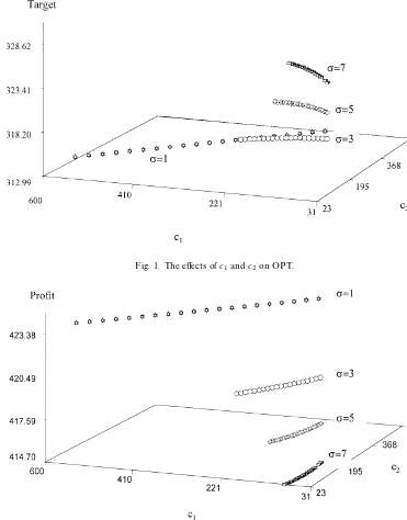
Fig. 1. The e!ects ofc
1andc2on OPT.
Fig. 2. The e!ects ofc
1andc2on expected pro"t.
where
c
1"(A1!(A2!S))/(cHp),
c
2"((A2!S)!A3)/(cHp),
c
3"(¸1!¸2)/p.
Figs. 1 and 2 display the e!ects of determining
the OPT and the expected pro"t for di!erent com-binations ofc
1andc2.c1andc2are chosen by using
the values of A
1,A2 and A3 and varying S as
described at the beginning of this section.c
1
Fig. 3. The e!ects ofc
1/c2on the loss. Fig. 4. The savings in terms of the varioususing process standard deviations of 1, 3, 5, and 7 mpf"xed holding costs,2.
from the original customer and the net revenue (selling price minus holding cost) from nonoriginal
customer in the primary market.c
2essentially
rep-resents the di!erence between the revenue from
a nonoriginal customer in the primary market and a customer in the secondary market. Fig. 1 provides the obvious, but very important, observation that the higher the process variability, the further away the optimal target is from the customer's speci" ca-tion limit. Fig. 2 conveys a useful fact that the higher the process variability, the lower the pro"t.
Fig. 3 emphasizes the e!ects ofc
1andc2on the
pro"tability. It shows the relationship between
the parameter ratio,c
1/c2, and the loss. In Fig. 3,
the loss is de"ned as the di!erence between the expected pro"t for placing the plant's target setting (i.e., 330 mpf2) and the expected pro"t from placing
of the OPT. The ratio,c
1/c2is described as
c
1
c
2
"A1!A2#S
A
2!A3!S
. (8)
Fig. 3 considers a case in which the process stan-dard deviation is 3 mpf2. A process standard
devi-ation of 3 mpf2was chosen because the real plant
data reveals this is a logical choice. It was also chosen because it has the same pattern as the other cases (i.e., where the standard deviations are 1, 5,
and 7 mpf2.) Fig. 3 indicates that the larger the
c
1/c2 ratio, the smaller the loss. Obviously, this
study seeks to decrease the loss and for this reason,
examines ways to obtain a largec
1/c2ratio. There
are two ways to achieve this. You can either
increase the value of the numerator or decrease the value of denominator in Eq. (8). Increasing the
numerator implies that the net revenue di!erence
between original and nonoriginal customers in the primary market should be large. As the net revenue
di!erence increases, there is a corresponding
decrease of the loss. This seems reasonable because the OPT would be further away from the cus-tomer's speci"cation limit. As a result, it leads to greater chances of the acceptability of the products, and it leads to a smaller loss. Decreasing the denominator in Eq. (8) also reduces the loss. This is because as the di!erence between net revenue in the primary and secondary markets gets smaller, there is no longer a bene"t in holding the product for sale in the primary market.
Turning now to Fig. 4, we can see how it displays the savings versus the various"xed holding costs, considering four levels of process variability (i.e., 1, 3, 5, and 7 mpf2, respectively). In this"gure, the
savings are expressed by taking the di!erence
between the expected pro"t from setting the OPT and the expected pro"t from setting the plant's
target at 330 mpf2. Two conclusions can be drawn
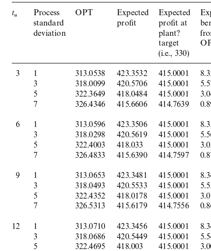
Table 2
The relationship amongt
u, process standard deviation, OPT,
and their corresponding expected pro"ts
t
u Processstandard
deviation
OPT Expected pro"t
Expected pro"t at plant? target (i.e., 330)
Expected bene"t from OPT
3 1 313.0538 423.3532 415.0001 8.3531 3 318.0099 420.5706 415.0001 5.5705 5 322.3649 418.0484 415.0001 3.0483 7 326.4346 415.6606 414.7639 0.8967 6 1 313.0596 423.3506 415.0001 8.3505 3 318.0298 420.5619 415.0001 5.5618 5 322.4003 418.033 415.0001 3.0329 7 326.4833 415.6390 414.7597 0.8793 9 1 313.0653 423.3481 415.0001 8.3480 3 318.0493 420.5533 415.0001 5.5532 5 322.4352 418.0178 415.0001 3.0177 7 326.5313 415.6179 414.7556 0.8623 12 1 313.0710 423.3456 415.0001 8.3455 3 318.0686 420.5449 415.0001 5.5448 5 322.4695 418.003 415.0001 3.0029 7 326.5786 415.5970 414.7514 0.8456
Fig. 5. Display of plant-loss when target settings range from 310 to 330 mpf2.
holding costs are. Similarly, in a case with the process's standard deviation of 7 mpf2, the savings decrease as the holding costs increase. This implies that the smaller the process variability, the #atter the slope, which leads to the process being more insensitive to the holding cost. All of this means that near constant savings can be achieved when there is small process variability. Thus, one can expect greater pro"t.
3.3. Variable holding cost
In addition to the parameters discussed above, some other parameters are needed to determine the OPT from Eq. (7). These parameters are arbitrarily selected as the values of the mean
holding time, t
u, ranging from 3 to 12 time
units, and the standard deviation of the holding
time, tp, ranging from 1 to 5 time units. The
"xed cost, a0, ranges from 10 to 50 units, and
the holding cost per unit time, a1, ranges from
1 to 5.
By using Newton}Raphson and Trapezoidal
Approximation, the solution of Eq. (7) can be
computed. Our "ndings suggest that the various
combinations ofa0anda1described above exhibit
the same basic pattern of e!ects on pro"tability. Likewise, the implications are similar for various
combination of thet
uandtp.
Table 2 shows the OPT values and their corre-sponding expected pro"t under various conditions. In Table 2, the expected bene"t from OPT is shown for average holding time 3}12 with 4 process stan-dard deviations.tpis equal to 1, a0is equal to 30, anda1is equal to 1 in this table. For example, in the
case of t
u"3 time units and p"3 mpf2, the
expected pro"t is $420.5706 when OPT is
318.0099 mpf2and the expected pro"t is$415.0001 when plant's target is set at 330 mpf2. This results in a bene"t of $5.5705 for using OPT. During a mass-production run, the total bene"t might be substantial.
Fig. 5 displays the corresponding `plant-lossa
when various target settings (TS) are made, ranging from 310 to 330 mpf2. The rest of the variables take on the values described above. Here, the plant-loss is de"ned as the di!erence between the expected pro"t for placing the plant's TS (i.e., 330 mpf2)
and the expected pro"t from placing of the speci"ed TS. Fig. 5 elicits three observations. The"rst obser-vation evinces how the loss is greatest when the
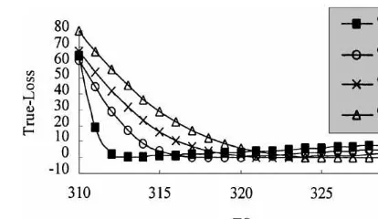
Fig. 6. Display of true-loss when target settings range from 310 to 330 mpf2.
is 7 mpf2. This is because, in this study, the cus-tomer's speci"cation is 310 mpf2. The process outputs would fall below 310 with a higher prob-ability when the process standard deviation is at the largest value. If process outputs were to fall below the customer speci"cation, then the pro-ducts would either sell to the market with the
price A
2 (with involvement of holding cost) or
sell to the secondary market with an even cheaper
price A3. As a result, when process outputs fall
below the customer's speci"cation, the loss is the greatest.
The second observation shows a case in which there is no plant-loss (i.e., the plant-loss equals 0). When no plant-loss is preferred, then the TS should be a larger value as process standard deviations increase. For example, in order to have the zero loss, the TS should be
approxi-mately 311.6 and 323.3 mpf2when standard
devi-ations are 1 and 7 mpf2, respectively. Fig. 5 shows how the slope is steeper when the TS is set at 311.6 mpf2for p"1 mpf2than it is when the TS is set to 323.3 mpf2 (for p"7 mpf2). A steeper
slope results in dramatic #uctuations in the
plant loss if the mean value shifts. The third observation deals with the fact that for all values of the process standard deviation, the plant loss approaches zero as the TS gets closer to 330 mpf2. This implies that the plant loss may be insensi-tive to the process variability when TS becomes large.
Fig. 6 presents the corresponding `true-lossa
when various target settings are made, ranging from 310 mpf2to 330 mpf2. True-loss is de"ned as the di!erence between the expected pro"t from setting OPT and the expected pro"t from setting the speci"ed TS. The results of Fig. 6 are similar to those of Fig. 5, with the one exception that the true-loss will not be the same when the TS increases. As the true-loss increases, the TS also increases. For example, when the TS is 330 mpf2, the lower the process variability is, the greater the true-loss is. Therefore, it seems reason-able to conclude that the determination of the OPT is important as long as the process remains in a stable state and lower process variability is maintained. If the OPT is found, the loss can be substantially reduced. In addition, the trend of
Figs. 5 and 6 addresses that the plant and true losses may be less sensitive to the process variabil-ity when the TS is large. This may explain the reason why the plant would have set a target of 330 mpf2.
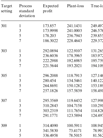
Table 3 sets out the trade-o! between product
rejection and the pro"tability. A lower TS has the advantage of lower production costs but the corre-sponding expected pro"ts are even lower. Table 3 shows the expected pro"t, plant-loss, and true-loss, respectively, when the TS ranges from 301 to
309 mpf2. Table 3 presents this information under
four conditions of the process standard deviations
ranging from 1, 3, 5, and 7 mpf2. Certainly when
one sets these lower TS values there is a very high chance of rejection of the product (i.e., the product quality is below the acceptable level). Here we wish only to demonstrate the potential savings this
process o!ers; but the potential saving is also a
Table 3
The relationship among process standard deviation, expected pro"t, plant-loss, and true-loss with target settings from 301 to 309
301 1 173.857 241.1431 249.4979 3 173.9998 241.0003 246.5764 5 178.203 236.7943 239.8553 7 186.3022 228.4643 229.3721 303 1 292.0894 122.9107 131.2655 3 236.6036 178.3965 183.9726 5 222.2988 192.6985 195.7595 7 221.5644 193.2021 194.1099 305 1 296.2088 118.7913 127.1461 3 280.454 134.5461 140.1222 5 264.8691 150.1282 153.1892 7 257.1826 157.5839 158.4917 307 1 295.3569 119.6432 127.9980 3 310.2843 104.7158 110.2919 5 303.2319 111.7654 114.8264 7 291.1771 123.5894 124.4972 309 1 314.4090 100.5911 108.9459 3 341.5830 73.4171 78.9932 5 336.4958 78.5015 81.5625 7 321.9554 92.8111 93.7189
equal 301, 307, and 309 mpf2. In this study, the
plant's speci"cation (¸
2) is 301 mpf2 and the
cus-tomer's speci"cation (¸
1) is 310 mpf2. When the
quality characteristic of the product is lower than the plant's speci"cation, then the selling price isA
3,
which is the lowest selling price. When the quality characteristic of the product is lower than the
cus-tomer speci"cation, then the selling price is
A
2which is lower than the primary priceA1.
There-fore, considering the case of TS of 301 mpf2, the
quality characteristic of the products would have
a higher probability to fall below 301 mpf2 when
the process standard deviation is small. This results in lower pro"t. The quality characteristic of the products would have a higher probability to fall
over 301 mpf2when the process standard deviation
is large. This could result in greater pro"t. Sim-ilarly, this feature works for the cases where the
values of TS are 307 and 309 mpf2. For example,
the quality characteristic of the products would
have a higher probability to fall below 310 mpf2
when the process standard deviation is 1 mpf2, and the quality characteristic of the products would
have a higher probability to fall over 310 mpf2
when the process standard deviation is larger. In-deed, this seems to suggest that when the process variability is large, so is the pro"t margin. In sum-mary, this study cautions against using values of TS
ranging from 301 to 309 mpf2 because even with
lower production costs there is still quite a high risk of loss.
4. Summary
This study has examined methods for determin-ing the optimal target settdetermin-ing for industrial pro-cesses in order to maximize expected pro"ts with respect to process variability and to production costs, material costs, holding costs, and other"scal considerations. Speci"c attention has been given to the determination of the optimal target setting in industries in which several grades of customer expectations are possible within the same market. In such circumstances, a manufacturer may hold products that have been rejected by the intended customer in the hopes of selling them to another customer in the same market. Even though the producer incurs a storage or holding cost, the net pro"t may still be higher than when the rejected goods are reworked, discarded, or sold in a second-ary market.
This study has examined such circumstances through mathematical modelling and through con-sideration of an actual case study. It presents methods for determining the optimal process target for an industrial process that considers the costs and bene"ts associated with holding rejected goods for later sale. It has also explored how these methods may be applied in the steel galvanization
industry. Our research "ndings show that the
key issue for greater pro"tability is low process variability.
The pivotal contribution of the present study is the recognition that the determination of a process
well as the bene"ts of holding rejected products for sale in the same market. Future research will
expand these e!orts to consider situations in
which holding costs are dependent on the distance from target. For the moment, it su$ces to conclude that it is reasonable for a manufacturer to set the process target close to the customer's speci" ca-tions when the process variability is low; a manu-facturer should be more conservative when confronting a higher process variability. Future research will also allow for the distribution of the holding time to be non-normal. Finally, future re-search will investigate how to extend the current
model to allow the value of ¸
2 to be a decision
Appendix B. The derivation of the5rst derivative of
E[P(x,t);u]
By using the results in Appendix A, we can obtain
dE[P(x,t);u] du
"(!A
1#A2!a0!a1BT)
A
!1
p
B
/A
¸
1!u
p
B
#(!A
2#A3#a0#a1BT)
A
!1
p
B
]/
A
¸2!up
B
!c. (B.1)Let m1"(¸
1!u)/p, and m2"(¸2!u)/p. Then
Eq. (B.1) can be derived as
dE[P(x,t);u]
du "k1/(m1)!k2/(m2)!c,
where
k
1"(1/p)(A1!A2#a0#a1BT),
k
2"(1/p)(A2!A3!a0!a1BT).
References
[1] R.G. Wilhelm, Controlling coating weight on a continuous galvanizing line, Control Engineering (1972) 44}47. [2] C.H. Springer, A method of determining the most
eco-nomic position of a process mean, Industrial Quality Con-trol 8 (1951) 36}39.
[3] D.C. Bettes, Finding an optimum target value in relation to a"xed lower limit and an arbitrary upper limit, Applied Statistics 11 (1962) 202}210.
[4] W.G. Hunter, C.P. Kartha, Determining the most pro" t-able target value of a production process, Journal of Qual-ity Technology 9 (1977) 176}181.
[5] L.S. Nelson, Best target values for a production process, Journal of Quality Technology 10 (1978) 88}89. [6] S. Bisgard, W.G. Hunter, L. Pallesen, Economic selection
of quality of manufactured product, Technometrics 26 (1984) 9}18.
[7] O. Carlsson, Determining the most pro"table process level for a production process under di!erent scales condition, Journal of Quality Technology 16 (1984) 44}49. [8] D.Y. Golhar, Determination of best mean contents for
a canning problem, Journal of Quality Technology 19 (1987) 82}84.
[9] D.Y. Golhar, S.M. Pollock, Determination of the optimal process mean and the upper limit for a canning problem, Journal of Quality Technology 20 (1988) 188}192. [10] D.Y. Golhar, Computation of the optimal process mean
and the upper limits for a canning problem, Journal of Quality Technology 20 (1988) 193}195.
[11] F.J. Arceleus, M.A. Rahim, Optimal process levels for the joint control of variables and attributes, European Journal of Operational Research 45 (1990) 224}230.
[12] F.J. Arceleus, M.A. Rahim, Simultaneous economic selec-tion of a variables and an attribute target mean, Journal of Quality Technology 26 (1994) 125}133.
[13] R.L. Schmidt, P.E. Pfeifer, Economic selection of the mean and upper limit for a canning problem with limited capacity, Journal of Quality Technology 23 (1991) 312}317.
[14] B.J. Melloy, Determining the optimal process mean and screening limits for packages subject to compliance testing, Journal of Quality Technology 23 (1991) 318}323. [15] T.O. Boucher, M.A. Jafari, The optimum target value for
single"lling operators with quality sampling plans, Jour-nal of Quality Technology 23 (1991) 44}47.
[16] J.S. Baxter, S.A. McClure, J.F. Forbes, Supervisory control of coating weight in galvanizing lines at Dofasco, Iron and Steel Engineer (1988) 17}22.