International Review of Economics and Finance 8 (1999) 267–280
Convergence of international output
Time series evidence for 16 OECD countries
Qing Li
a,*, David Papell
baDepartment of Economics, Wichita State University, Wichita, KS 67260-0078, USA bDepartment of Economics, University of Houston, Houston, TX 77204-5882, USA
Received 27 January 1998; accepted 18 June 1998
Abstract
This article examines convergence of per capita output for 16 OECD (Organization for Economic Cooperation and Development) countries. Conventional tests on conditional and time series convergence have given mixed results for similar economies. Utilizing the concepts of deterministic and stochastic convergence, we develop techniques which incorporate endoge-nously determined break points to test the unit root hypothesis in relative per capita income. The tests provide evidence of deterministic convergence for 10, and stochastic convergence for 14, of the 16 OECD countries. Our findings reveal that World War II is the major cause of the structural shifts in relative output. 1999 Elsevier Science Inc. All rights reserved.
JEL classification:C32; O40
Keywords:Stochastic convergence; Deterministic convergence; ADF test
1. Introduction
Convergence, the tendency for per capita income of different economies to equalize over time, is one of the predictions of Solow’s (1956) neoclassical growth model. Over the past decade, much theoretical and empirical work has been done in this area. The implications of convergence, or lack of convergence, for long-run relationships between different countries has led to a surge of interest and debate.
Solow’s model predicts that convergence exists among different economies regard-less of initial conditions once the determinants of aggregate production functions are
* Corresponding author. Tel.: 316-978-3220; fax: 316-978-3308.
E-mail address: [email protected] (Q. Li)
controlled for. It therefore requires a negative correlation between initial per capita output and its growth rate, so that poorer countries will catch up with wealthier countries. Pioneered by Baumol (1986), numerous studies exploring convergence have been developed. While Romer (1986) and Delong (1988) challenge the hypothesis of cross-country convergence, Barro (1991) and Mankiw, Romer, and Weil (1992) find that convergence can be achieved among economies that exhibit similar characteristics and when human capital variables such as education and savings rates are controlled for. They refer to this cross-section notion of convergence as conditional convergence. Another form of convergence examines long-run output movements. Bernard and Durlauf (1995) define convergence between two (or more) countries when the long-run forecasts of output differences tend to zero as the forecasting horizon tends to infinity. Tests for the time series notion of convergence require cross-country per capita output differences to be stationary. In the bivariate case, this requires that the outputs be cointegrated with cointegrating vector [1,21]. We refer to this notion of convergence as time series convergence. If they are cointegrated with cointegrating vector [1,2l], there are common trends in output. Thus cointegration between econo-mies is a necessary, but not a sufficient condition for convergence.
The time series evidence has not been supportive of the convergence hypothesis. Quah (1990) and Ben-David (1994) do not find general evidence of convergence among a large number of countries using the Summers-Heston (1988) data.1Campbell and Mankiw (1989) fail to find convergence among OECD countries which display similar economic characteristics. Bernard and Durlauf (1995), in a study of 15 OECD countries from 1900 to 1987, reject convergence but find substantial evidence of common trends.2
Although these two testing frameworks have contributed to our understanding of the growth process, they also are the cause of confusion among different studies. Bernard and Durlauf (1996) show that conditional convergence is a weaker notion of convergence than time series convergence. They find that cross-section tests tend to spuriously reject the null of no convergence when economies have different long run steady states and that failure to reject the no convergence null using time series tests can be due to transitional dynamics in the data.
Because the time series tests for convergence depend on unit root and cointegration tests which are known to have relatively more power using data over a long time period, it is important to develop an economic framework that incorporates potential structural change in the deterministic component of the trend function. Failure to do so might lead to bias towards the acceptance of no convergence and to an erroneous interpretation of output movements.
Carlino and Mills (1993) are interested in regions of the United States, and so consider regional per capita income relative to the United States as a whole. They adopt conventional Augmented-Dickey-Fuller (ADF) tests, which fail to reject the unit root hypothesis in the log of relative regional per capita output for all eight U.S. regions. They then incorporate an exogenously imposed trend break into the tests and are able to reject the unit root null for three out of eight regions, providing some evidence of stochastic convergence. Loewy and Papell (1996) reexamine the issue by allowing endogenously determined break points and lag lengths. They are able to find evidence of stochastic convergence in seven out of eight U.S. regions, which signifi-cantly strengthens Carlino and Mills’ results and provides a benchmark case for convergence among similar economies.
We examine the unit root hypothesis in relative per capita income for 16 OECD economies from 1900 to 1989. Using both conventional ADF tests and Perron’s (1997) sequential tests for unit roots with endogenously determined trend breaks to investigate Carlino and Mills’ (1993) notion of stochastic convergence, we are able to reject the unit root hypothesis in 14 out of 16 countries. We also test for deterministic conver-gence. Using ADF and Perron and Vogelsang’s (1992) tests with endogenously deter-mined breaks in the mean, as well as tests, developed below, which force the break to eliminate the deterministic trend, we are able to reject the unit root hypothesis in 10 of the 16 countries. By incorporating structural change and considering stochastic, as well as deterministic, convergence, we are able to find more evidence of convergence than found by Bernard and Durlauf (1995).
2. Empirical results
Time series notions of convergence imply that per capita output disparities between converging economies follow a stationary process. Stochastic or deterministic conver-gence is therefore directly related to the unit root hypothesis in relative per capita output. We utilize both conventional ADF tests as well as tests which incorporate a one-time break in the deterministic trend. Rejection of the null hypothesis of a unit root, whether or not a break is included, provides evidence of convergence. Whether it constitutes evidence of stochastic or deterministic convergence depends on the exact form of the test.
The data are from Maddison (1991), adjusted to exclude the impact of boundary changes. Per capita GDPs are calculated by dividing aggregate GDPs by mid-year population levels. While the Maddison data begins in 1870 and ends in 1989, we truncate the data before 1900 since the data in the prior years are of lower quality and are not available for Japan, the Netherlands and Switzerland. By using the more recent Maddison data, we are able to add one additional country (Switzerland) and two more years to the data analyzed by Bernard and Durlauf (1995).
DRIt5 m 1 bt1 aRIt211
o
k
j51
cjDRIt2j1 et, (1)
whereRItstands for the logarithm of relative per capita output of individual country
at timet, which is measured by individual country’s per capita output as a percentage of the aggregate per capita output of the group. Specifically, we take the logarithm of the individual country’s per capita real GDP divided by the aggregate per capita real GDP, which is calculated by dividing the aggregate real GDP of all 16 countries by the total population of these countries.
We use a data dependent method to select the value ofk.Following Campbell and Perron (1991), we first start with an upper bound, kmax(8 in this case), on k. If the t-statistic on kth lagged first differences DRI is significant, choose k 5 kmax. If not, reducekby one until the last included lag becomes significant. If no lags are significant, we set k 50. We use the 10% value of the asymptotic normal distribution (1.6) as the significance criterion. We are able to reject the unit root hypothesis in favor of a trend stationary alternative if a is significantly different from zero. In that case, stationarity of relative per capita output constitutes evidence of stochastic convergence. We also run the ADF without a time trend. In that case, rejection of the unit root hypothesis in favor of the alternative of level stationarity constitutes evidence of deterministic convergence.
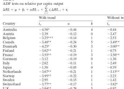
The results from the ADF tests are reported in Table 1. With a time trend, the unit root hypothesis can be rejected at the 5% level for nine of the 16 countries. Without a time trend, the null is rejected for five countries. Even without a trend break, we are able to find considerable evidence for stochastic convergence, and some evidence for deterministic convergence.
Although the ADF is the standard methodology for testing the unit root hypothesis, there is much evidence that it has serious power problems. As emphasized by Campbell and Perron (1991), misspecification of the deterministic trend can bias test results towards the nonrejection of the unit root hypothesis. This is especially important in the case of long time spans of data which are likely to be affected by major structural shifts. On the other hand, in the absence of a trend break allowing for structural change, as in the sequential Dickey-Fuller tests described below, will decrease the power of the tests.
Sequential Dickey-Fuller tests which allow for a one-time change in both the inter-cept and the slope of the deterministic trend, with the time of break determined endogenously, have been developed by Banerjee, Lumsdaine, and Stock (1992), Chris-tiano (1992), and Zivot and Andrews (1992). We use the specification in Perron (1997).5 The model is an example of an “innovational outlier” model because the change is assumed to occur gradually. The sequential ADF test involves estimating the following regressions which are given in Eq. (2):
DRIt5 m 1 bt1 dD(TB)t1 uDUt 1 gDTt 1 aRIt211
o
k
j51
cjDRIt2j1 et, (2)
Table 1
ADF tests on relative per capita output DRIt5 m 1 bt1 aRIt211
o
k
j51
cjDRIt2j1 et
With trend Without trend
Country ta a k ta a k
Australia 24.56* 20.44 4 20.44 20.01 7
Austria 22.39 20.12 0 22.47 20.12 0
Belgium 23.25*** 20.14 1 22.53 20.08 1
Canada 23.48** 20.24 5 23.49** 20.23 5
Denmark 24.25* 20.30 3 23.00** 20.16 1
Finland 23.62** 20.21 1 20.75 20.03 4
France 23.55** 20.19 3 23.56** 20.19 3
Germany 23.12 20.19 0 21.36 20.05 0
Italy 22.62 20.11 1 22.49 20.10 1
Japan 21.50 20.05 0 20.39 20.01 0
Netherlands 23.67** 20.21 1 23.15** 20.16 1
Norway 23.95** 20.22 1 22.23 20.08 1
Sweden 22.95 20.15 1 21.43 20.05 5
Switzerland 23.77** 20.17 1 23.82* 20.17 1
U.K. 23.64** 20.28 5 20.92 20.02 6
U.S. 22.03 20.08 4 20.56 20.01 4
Critical values forta
1% 5% 10%
With trend 4.05 3.46 3.15
Without trend 3.50 2.89 2.58
* denotes statistical significance at the 1% level. ** denotes statistical significance at the 5% level. *** denotes statistical significance at the 10% level.
Critical values are from MacKinnon (1991) with 90 observations.
otherwise, the “intercept” dummy DUt 5 1 if t . TB, 0 otherwise, and the “slope”
dummyDTt5t2TBift.TB, 0 otherwise. With the break date chosen exogenously,
this is the test in Perron (1989). In order to endogenize the break date selection, we run different regressions forTB52, 3, . . . ,T–1. The break date is chosen to minimize
the t-statistic on a. The unit root null is rejected in favor of trend stationarity, and hence evidence is provided for stochastic convergence, ifa is significantly different from zero. We use the same technique as described above for the ADF test to choose the lag length.6
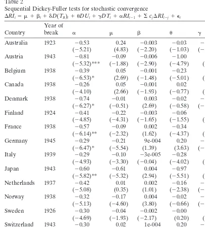
The results for the sequential Dickey-Fuller tests are presented in Table 2. Incorpo-rating trend breaks in the unit root tests significantly strengthens the findings of stochastic convergence. Using Perron’s (1997) finite sample critical values for T 5
Table 2
Sequential Dickey-Fuller tests for stochastic convergence
DRIt5 m 1 bt1 dD(TB)t1 uDUt1 gDTt1 aRIt211 ScjDRIt2j1 et Year of
Country break a m b u g d k
Australia 1923 20.53 0.24 20.003 20.03 20.001 0.04 4
(25.21) (4.83) (22.20) (21.03) (20.25) (1.14)
Austria 1943 20.81 20.09 20.006 21.00 0.017 0.25 8
(25.32)*** (21.88) (22.90) (24.79) (4.55) (2.23)
Belgium 1938 20.39 0.05 20.001 20.23 0.002 0.13 1
(26.53)* (2.69) (21.48) (25.01) (2.81) (2.60)
Canada 1938 20.26 0.05 20.001 0.02 0.001 20.07 2
(24.10) (2.66) (21.93) (20.77) (0.90) (21.70)
Denmark 1938 20.74 20.01 0.003 20.02 20.003 0.15 8
(26.27)* (20.51) (2.69) (20.58) (22.64) (2.73)
Finland 1924 20.41 20.22 20.003 20.06 0.005 20.02 3
(24.85) (24.31) (21.65) (21.55) (2.52) (20.48)
France 1938 20.57 20.09 0.002 20.34 0.003 0.24 8
(26.14)** (22.32) (1.62) (24.37) (1.65) (2.95)
Germany 1945 20.29 20.21 9e-004 0.20 20.001 20.69 1
(26.47)* (25.54) (1.39) (3.63) (21.07) (211.1)
Italy 1939 20.29 20.10 23e-005 20.28 0.004 0.08 1
(24.93) (23.30) (20.04) (24.02) (3.18) (1.18)
Japan 1943 20.60 20.61 0.004 20.97 0.014 0.23 8
(25.82)** (25.32) (2.94) (25.51) (5.22) (2.41)
Netherlands 1937 20.42 0.01 0.002 20.16 20.001 0.12 3
(25.08) (0.35) (1.01) (22.38) (20.10) (1.32)
Norway 1938 20.32 20.17 0.004 20.02 20.001 0.05 1
(25.13) (24.60) (3.80) (20.66) (21.53) (0.99)
Sweden 1926 20.30 20.04 20.002 20.00 0.003 20.06 1
(24.69) (21.93) (22.17) (0.20) (2.31) (21.52)
Switzerland 1943 20.30 0.02 1e-004 0.20 20.003 20.12 1
(25.83)** (1.56) (0.24) (4.49) (23.18) (22.44)
U.K. 1928 20.33 0.15 20.004 0.01 0.001 20.04 3
(24.46) (4.04) (23.51) (0.45) (0.50) (21.11)
U.S. 1938 20.36 0.21 20.002 0.16 20.002 20.06 8
(25.96)** (6.02) (23.04) (4.65) (22.82) (21.96) Critical values forta
1% 5% 10%
26.21 25.55 25.25
* denotes statistical significance at the 1% level. ** denotes statistical significance at the 5% level. *** denotes statistical significance at the 10% level.
country, Austria.7 Some of the nonrejections appear to be caused by the decreased power of the sequential Dickey-Fuller test in the absence of a trend break. Of the remaining eight countries, the unit root null can be rejected at the 5% level by the ADF test in six cases.
The ADF and sequential Dickey-Fuller tests together provide strong evidence in support of stochastic convergence for the 16 OECD countries. The only two countries for which we are unable to reject the unit root null at the 5% level in either test are Italy and Sweden. Therefore, for 14 out of 16 OECD countries, we are able to reject the unit root hypothesis, a result that provides us with evidence of stochastic convergence.8
Testing for a unit root in relative per capita income is only an interesting question if at least some of the individual series are nonstationary. If all of the individual series were stationary, the relative series would necessarily be stationary.9 We conducted, but do not report, ADF and sequential Dickey-Fuller tests on the individual series. In the absence of breaks, the unit root null cannot be rejected by the ADF test for any country. With breaks, the null can be rejected in half of the cases, but with a wide variety of break dates.10
The trend breaks and dummy variables contain economic implications. By examin-ing the coefficients of the dummies, most of the 16 countries can be put into two categories: those which are characterized by an initial fall in output (indicated by a negative sum of the one-time and intercept dummies), and a faster growth rate after-wards (indicated by a positive slope dummy), and those which are characterized by an initial rise in output (a positive sum of the one-time and intercept dummies), followed by a slower growth (a negative slope dummy).
The trend breaks for per capita relative output mostly take place around World War II. Austria, Germany, Japan and Switzerland experience breaks around the end of the war, while Belgium, Canada, Denmark, France, Italy, the Netherlands, Norway and the United States have breaks at the beginning of the war. In their study of per capita output for the same countries, Ben-David and Papell (1995) find that the Great Depression instead of World War II is the cause of the breaks for the United States and Canada. The different impact of the two events on these countries may explain the discrepancy. Unlike World War II, the Great Depression affected almost every industrialized country, it therefore fails to induce breaks inrelativeper capita output. Twelve of the 16 countries experience breaks around World War II. Most display an initial fall in output, followed by a higher growth rate. The United States, which was relatively unaffected by the war, is an exception. Per capita output for the United States (relative to the group) initially rises with the onset of the war, followed by slower (relative) growth. Breaks occur in the 1920s for Australia, Finland, Sweden, and the United Kingdom. In Australia, World War I brought shortages of goods which led to postwar industrial expansion. Finland’s break can be explained by its independence from the Soviet Union in 1920 and the subsequent civil war. The United Kingdom’s break occurs in 1928, shortly after a wave of strikes culminated in the general strike of 1926.
separates Sweden from the rest of the world is its longtime political neutrality. During World War II, Sweden was the only Scandinavian country to succeed in remaining neutral, and emerged from both wars virtually undamaged. Its break date of 1926 can be explained by widespread unemployment during the recession in the 1920s.
We now consider deterministic convergence, the type of time series convergence defined and tested by Bernard and Durlauf (1995). Deterministic convergence requires that the log of relative output be level stationary, and is hence considered to be a stronger notion of time series convergence than stochastic convergence. We test the unit root hypothesis in relative per capita income allowing a structural change in the mean. Based on Perron and Vogelsang (1992), we estimate the following equation:
DRIt5 m 1 dD(TB)t1 uDUt1 aRIt211
o
k
j51
cjDRIt2j1 et, (3)
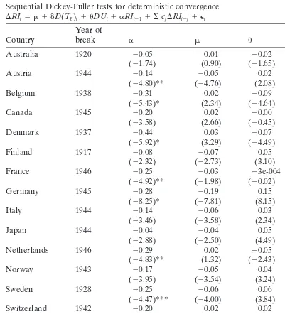
Eq. (3) differs from Eq. (2) by excluding the time trend and the trend dummy variable. Perron and Vogelsang (1992) compute finite sample critical values forT5100, with the lag length chosen as described before. The results are shown in Table 3. The unit root null can be rejected in favor of the level stationary alternative at the 5% level for six out of 16 countries: Austria, Belgium, Denmark, France, Germany, and the Netherlands; and at the 10% level for two additional countries, Sweden and Switzer-land.11 In the absence of a break, the unit root null can also be rejected at the 5% level by the ADF test for Canada. With the unit root null being rejected for over half of the countries, this result provides considerable, but by no means universal, evidence of deterministic convergence.
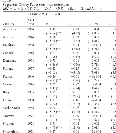
The concept of deterministic convergence requires the elimination of the determinis-tic, as well as the stochasdeterminis-tic, trend. An alternative test of deterministic convergence consists of testing for a unit root in Eq. (2) under the restriction that the trend break eliminates the deterministic trend. This involves estimating sequential Dickey-Fuller tests for Eq. (2) withb 1 g 50. If the null hypothesis of a unit root can be rejected, convergence will be to a zero postbreak trend, and hence the conditions for determinis-tic convergence will be satisfied.
The critical values for this test are different from the two tests described above and have not, to our knowledge, been tabulated. Following Perron and Vogelsang (1992) and Perron (1997), we consider the random walk data generating process for our sample size of 90 observations as given in Eq. (4).
yt5yt211 et, (4)
withy050 andetto be i.i.d.N(0,1). Our test statistic is thet-statistic onain Eq. (2),
under the restriction thatb 1 g 5 0, with the lag lengthkfor each series chosen as described above. Repeating this process 5000 times, the critical values for the finite sample distributions are obtained from the sorted vector of the replicated statistics.
Table 3
Sequential Dickey-Fuller tests for deterministic convergence DRIt5 m 1 dD(TB)t1 uDUt1 aRIt211 ScjDRIt2j1 et
Year of
Country break a m u d k
Australia 1920 20.05 0.01 20.02 0.09 7
(21.74) (0.90) (21.65) (2.77)
Austria 1944 20.14 20.05 0.02 20.85 4
(24.80)** (24.76) (2.08) (217.5)
Belgium 1938 20.31 0.02 20.09 0.08 1
(25.43)* (2.34) (24.64) (1.57)
Canada 1945 20.20 0.02 20.00 0.12 2
(23.58) (2.66) (20.45) (3.20)
Denmark 1937 20.44 0.03 20.07 0.14 3
(25.92)* (3.29) (24.49) (2.78)
Finland 1917 20.08 20.07 0.05 20.20 7
(22.32) (22.73) (3.10) (23.86)
France 1946 20.25 20.03 23e-004 20.41 3
(24.92)** (21.98) (20.02) (23.98)
Germany 1945 20.28 20.19 0.15 20.68 1
(28.25)* (27.81) (8.15) (211.1)
Italy 1944 20.14 20.06 0.03 20.22 1
(23.46) (23.58) (2.34) (23.09)
Japan 1944 20.04 20.04 0.05 20.66 1
(22.88) (22.50) (4.49) (214.23)
Netherlands 1946 20.29 0.02 20.05 20.45 1
(24.83)** (1.32) (22.43) (23.29)
Norway 1943 20.17 20.05 0.04 20.12 1
(23.95) (23.54) (3.24) (22.27)
Sweden 1928 20.25 20.06 0.06 20.04 1
(24.47)*** (24.00) (3.84) (21.10)
Switzerland 1942 20.20 0.02 0.02 20.10 1
(24.39)*** (2.06) (1.57) (22.05)
U.K. 1940 20.09 0.02 20.03 0.03 6
(22.60) (1.75) (22.56) (0.68)
U.S. 1958 20.13 0.06 20.04 0.03 1
(23.05) (2.92) (22.87) (1.00)
Critical values forta
1% 5% 10%
25.33 24.58 24.27
* denotes statistical significance at the 1% level. ** denotes statistical significance at the 5% level. *** denotes statistical significance at the 10% level.
Table 4
Sequential Dickey-Fuller tests with restrictions
DRIt5 m 1 bt1 dD(TB)t1 uDUt1 gDTt1 aRIt211 ScjDRIt2j1 et Restriction:b 1 g 50
Year of
Country break a m b(2g) u d k
Australia 1974 20.49 0.23 20.004 20.29 0.04 4
(24.94)*** (4.73) (24.80) (24.84) (1.26)
Austria 1944 20.16 20.03 20.001 20.01 20.85 4
(25.20)** (21.47) (21.81) (20.53) (217.8)
Belgium 1938 20.33 0.04 29e-004 20.12 0.08 1
(25.58)** (2.18) (21.21) (24.20) (1.63)
Canada 1916 20.24 20.00 0.004 0.02 0.07 2
(23.98) (20.12) (1.52) (0.78) (2.04)
Denmark 1938 20.73 20.01 0.003 20.04 0.15 8
(26.46)* (20.56) (2.71) (21.38) (2.80)
Finland 1977 20.22 20.15 0.001 0.12 20.03 1
(23.65) (23.45) (3.01) (3.35) (20.64)
France 1946 20.26 20.01 28e-004 20.02 20.41 3
(24.93)*** (20.26) (20.77) (20.65) (23.93)
Germany 1945 20.29 20.22 9e-004 0.19 20.69 1
(28.41)* (26.74) (1.44) (6.70) (211.2)
Italy 1955 20.19 20.05 20.001 0.00 20.03 1
(23.71) (22.06) (21.98) (0.07) (20.50)
Japan 1958 20.12 20.10 22e-004 0.09 20.06 0
(22.72) (22.32) (20.34) (2.55) (20.68)
Netherlands 1946 20.32 0.06 20.002 20.09 20.44 1
(25.05)*** (1.85) (21.41) (22.56) (23.24)
Norway 1977 20.23 20.09 9e-004 0.10 20.02 1
(24.03) (23.47) (2.67) (3.28) (20.37)
Sweden 1928 20.31 20.04 20.002 0.04 20.06 1
(24.98)*** (22.40) (22.01) (2.09) (21.42)
Switzerland 1973 20.27 0.01 7e-004 20.00 0.06 1
(25.02)*** (0.99) (2.42) (20.28) (1.33)
U.K. 1964 20.23 0.09 20.002 20.13 0.02 3
(23.54) (3.16) (23.15) (23.35) (0.48)
U.S. 1958 20.13 0.06 24e-005 20.04 0.03 1
(23.02) (2.83) (20.16) (22.59) (0.99) Critical values forta
1% 5% 10%
25.67 25.12 24.80
* denotes statistical significance at the 1% level. ** denotes statistical significance at the 5% level. *** denotes statistical significance at the 10% level.
for Australia, France, Netherlands, Sweden, and Switzerland. These generally accord with the previously reported results for deterministic convergence, although the rejec-tions for several of the countries are at lower significance levels. The rejection of the unit root null for Australia was not found above, and provides additional evidence of deterministic convergence.
3. Conclusions
The neoclassical growth theory originated by Solow (1956) has sparked many empiri-cal efforts to determine the long run behavior of different countries. A large literature on convergence across economies has produced a diverse body of testing methodolo-gies as well as definitions. While most convergence studies focus on testing the cross-section version of convergence, referred to as conditional convergence, Bernard and Durlauf (1996) find that the time series version is a stronger notion of convergence. Bernard and Durlauf (1995) use time and frequency domain approaches to examine persistence in per capita output deviations, and fail to find evidence of deterministic convergence for 15 OECD countries. We employ time series techniques which incorpo-rate structural breaks to explore both deterministic and stochastic convergence among 16 OECD countries. In particular, we test the unit root hypothesis on the log relative per capita output (to that of the group). If we find evidence against the unit root null for its relative per capita output, a country’s output is converging to the aggregate output of the whole group.
We find considerable evidence of convergence among the 16 OECD countries. Combining tests with and without structural breaks, we can reject the unit root null against an alternative of trend stationarity, and thus provide evidence for stochastic convergence, for 14 of the 16 countries. We can also reject the unit root null in favor of a level stationary alternative, and provide evidence of deterministic convergence, for 10 of the 16 countries. The results of the sequential unit root tests also reveal that World War II is the major cause for the structural shifts of relative per capita outputs.
Acknowledgments
We are grateful to Andrew Bernard, Dan Ben-David, Michael Loewy, and Kei-Mu Yi for helpful comments and discussions.
Notes
1. Ben-David (1994) finds some evidence in support of Baumol’s finding of a convergence club among both the world’s wealthiest countries and among the world’s poorest countries.
The combined results provide some evidence of deterministic cointegration among most OECD countries.
3. This terminology corresponds to Ogaki and Park’s (1998) definition of stochastic cointegration when the stochastic trend components of the (two or more) series are cointegrated, and deterministic cointegration when both the stochastic and deterministic trends are eliminated by the cointegrating vector.
4. Bernard and Durlauf (1991) report that allowing for a constant difference in logs did not markedly change their results.
5. These tests all restrict breaks to one-time changes. Unit root tests which allow for two breaks have been developed by Lumsdaine and Papell (1997) and applied to long-term international output by Ben-David, Lumsdaine, and Papell (1997).
6. Ng and Perron (1995) discuss the advantages of this recursivet-statistic method over an alternative procedure where k is chosen to minimize the Akaike Infor-mation Criterion.
7. Since we have 90 observations, using critical values withT5100 could poten-tially cause us to inappropriately reject the unit root null. Perron (1997) also provides critical values for T 5 70. The only difference is that the null for Denmark is rejected at the 5%, rather than the 1%, level. The critical values incorporate the lag length selection methods. They are considerably lower, and hence more conservative, than either asymptotic critical values or finite sample critical values which fix the value of k.
8. For any given version of the tests, however, we can reject the unit root null for only about one-half of the countries.
9. If the output series are trend stationary, convergence requires that the time trends for each country’s output must be the same.
10. In the absence of breaks, Ben-David and Papell (1995), using the Maddison data for individual countries extended back to 1870, can only reject the unit root null at the 5% level for the United States. With breaks, they can reject the null for 11 countries, but only nine of these remain significant with finite sample critical values.
11. Perron and Vogelsang (1992) also tabulate critical values for T550, a much smaller number than our 90 observations. The only difference from using these critical values is that the null is no onger rejected for Switzerland. This makes no difference for the convergence results because, using the ADF test, the null for Switzerland can be rejected at the 1% level.
12. In order to provide a comparison with previous work, we also simulated critical values with T 5100. The results were very close to those withT 590.
References
Barro, R. J. (1991). Economic growth in a cross-section of countries.Quarterly Journal of Economics 106, 407–443.
Baumol, W. J. (1986). Productivity growth, convergence, and welfare.American Economic Review 76, 1072–1085.
Ben-David, D. (1994). Convergence Clubs and Diverging Economies. CEPR Discussion Paper, 922. Ben-David, D., Lumsdaine, R. L., & Papell, D. H. (1997). The Unit Root Hypothesis in Long-Term Output:
Evidence from Two Structural Breaks for 16 Countries. Working Paper, University of Houston. Ben-David, D., & Papell, D. H. (1995). The Great Wars, the Great Crash and steady state growth: some
new evidence about an old stylized fact.Journal of Monetary Economics 36, 453–475.
Bernard, A. B., & Durlauf, S. N. (1991). Convergence of International Output Movements. NBER Working Paper, 3717.
Bernard, A. B., & Durlauf, S. N. (1995). Convergence of international output. Journal of Applied Econometrics 10, 97–108.
Bernard, A. B., & Durlauf, S. N. (1996). Interpreting tests of the convergence hypothesis.Journal of Econometrics 71, 161–174.
Campbell, J. Y.,& Mankiw, N. G. (1989). International evidence on the persistence of economic fluctua-tions.Journal of Monetary Economics 23, 319–333.
Campbell, J. Y., & Perron, P. (1991). What macroeconomists should know about unit roots. In O. Blanchard & S. Fischer (Eds.),NBER Macroeconomics Annual(pp. 141–201). Cambridge, MA: MIT Press.
Carlino, G. A., & Mills, L. O. (1993). Are U.S. regional incomes converging? A time series analysis.
Journal of Monetary Economics 32, 335–346.
Christiano, L. (1992). Searching for a break in GNP.Journal of Business and Economic Statistics 10, 237–250.
DeLong, J. B. (1988). Productivity growth, convergence, and welfare: comment.American Economic Review 78, 1138–1154.
Li, Q, (1994). Cointegration of International Output Movements: the Case of OECD Countries. Working Paper, Wichita State University.
Loewy, M. B., & Papell D. H. (1996). Are U.S. regional incomes converging? Some further evidence.
Journal of Monetary Economics 38, 587–598.
Lumsdaine, R. L., & Papell D. H. (1997). Multiple trend breaks and the unit root hypothesis.Review of Economics and Statistics 79, 212–218.
MacKinnon, J. (1991). Critical values for cointegration tests. In R. F. Engle & C. W. J. Granger (Eds.),
Readings in Cointegration(pp. 267–276). New York: Oxford University Press.
Maddison, A. (1991).Dynamic Forces in Capitalist Development: A Long-Run Comparative View.Oxford: Oxford University Press.
Mankiw, N. G., Romer, D., & Weil, D. N. (1992). A contribution to the empirics of economic growth.
Quarterly Journal of Economics 107, 407–438.
Ng, S., & Perron, P. (1995). Unit root tests in ARMA models with data dependent methods for the selection of the truncation lag.Journal of the American Statistical Association 90, 268–281.
Ogaki, M., & Park, J. Y. (1998). A cointegration approach to estimating preference parameters.Journal of Econometrics 82(1), 107–134.
Perron, P. (1989). The Great Crash, the oil price shock, and the unit root hypothesis.Econometrica 57, 1361–1401.
Perron, P. (1994). Trend, unit root and structural change in macroeconomic time series. In B. B. Rao (Ed.),Cointegration for the Applied Economist(pp. 113–140). New York: St. Martin’s.
Perron, P. (1997). Further evidence on breaking trend functions in macroeconomic variables.Journal of Econometrics 80, 355–385.
Perron, P., & Vogelsang, T. (1992). Nonstationarity and level shifts with an application to purchasing power parity.Journal of Business and Economic Statistics 10, 301–320.
Romer, P. (1986). Increasing returns and long run growth.Journal of Political Economy 94, 1002–1037. Solow, R. M. (1956). A contribution to the theory of economic growth.Quarterly Journal of Economics
70, 65–94.
Summers, R., & Heston, A. (1988). A new set of international comparisons of real product and price levels estimates for 130 countries, 1950–1985.Review of Income and Wealth 34, 1–25.