A NEW RELIABLE BORESIGHT CALIBRATION METHOD
FOR MOBILE LASER SCANNING APPLICATIONS
R. Le Scouarnecb, *, T. Touzé a, J.B. Lacambreb, N. Seube a
a ENSTA Bretagne, Dept STIC/OSM, Brest - (nicolas.seube, thomas.touzé)@ensta-bretagne.fr b
iXBlue, Marly-le-roi, (romain.le-scouarnec, jean-baptiste.lacambre)@ixblue.com
KEY WORDS: Mobile laser scanning, Calibration, Boresight, Positioning-free, Plane features.
ABSTRACT:
This paper presents a new INS-LiDAR bore-sighting parameters calibration method that differs from traditional methods on two main aspects. First, the method is static, which avoids being affected by GPS errors and enables the extraction of scanlines. For terrestrial laser scanning, this aspect is extremely important since ranges are short and the GPS errors are the first source of error during the calibration process. Second, the method is based on a rigorous mathematical model, which allows providing reliable boresight quality factors. After presenting the boresight determination problem, this paper will introduce the existing calibration procedures. Then, it will describe the new procedure and explain how it overcomes the limitations of the traditional approaches. Finally, some results from both simulations and real datasets are presented to illustrate our approach.
Corresponding author.
1. INTRODUCTION
1.1 The INS-LiDAR system
A mobile laser scanning system is composed by a LiDAR which gives the distance to the target, an INS that provides the system orientation and a GNSS that estimates the position in a global frame. Combined altogether, these 3 instruments enable the geolocalization of the LiDAR points in a global frame such as the [ECEF] frame (Earth Centered Earth fixed).
A geo-location equation for this system is:
INS
IN
ecef ecef ecef n INS LiDAR n LiDAR LiDAR LiDAR GPSC C S C
X X b X (1)
Where Measurements:
LiDAR LiDAR
X : Range measured by the LiDAR in [LiDAR] frame
ecef GPS
X : GPS antenna position
n INS
C : Rotation matrix calculated thanks to the INS data
ecef n
C : Rotation matrix from [n] to [ECEF]
Parameters to be calibrated:
LiDA S
R IN
C : Rotation matrix from [LiDAR] frame to [INS] frame
INS
b : Lever arm between the LiDAR and the GPS antenna
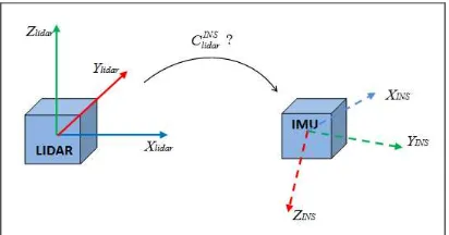
Boresight calibration consists in determining the relative orientation of the LiDAR to the INS described by LiDAS
R IN
C .
Figure 1: Relative orientation between LiDAR and INS
For terrestrial laser scanning, the error due to the boresight should be inferior to the cm-level in order to be lower to positioning uncertainty, which is less than 1cm with INS/GNSS hybridized post-processed data.
At a given range, the shift error εboresight created by a boresight error θboresight can be approximated by this expression:
εboresight[m]=Range[m]⨯θboresight.
Therefore with a 50 meter range, θboresight needs to be inferior to 10-2 degree in order to get an error εboresight inferior to 1cm.
Mechanically, it is difficult to know precisely the relative orientation of the LiDAR to the INS, i.e., CLiDAINSRis known within about a few degrees. Then, the remaining misalignment needs to be estimated computationally via a calibration procedure. Mathematically, the misalignment can be modeled by a rotation matrix *
S INS IN
C called boresight matrix.
* * INS INS INS LiDAR INS LiDAR
C C C
Where LiDA S
R IN
C : “true” relative orientation
* INS LiDAR
C : Approximate mechanical relative orientation
[INS] can be defined as the “true” INS frame whereas [INS* ] is the approximate INS frame resulting from the approximate
rotationCLiDARINS* .
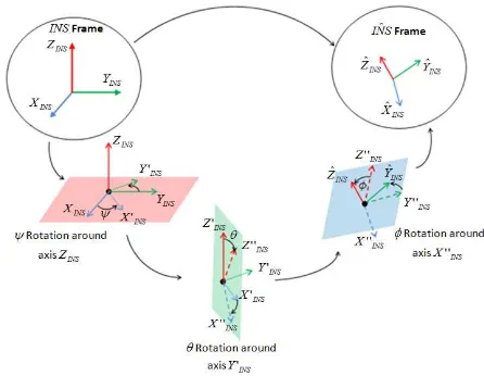
The Boresight matrix * S INS IN
C is characterized by the 3 boresight
angles. These boresight angles are defined in the figure 2.
Figure 2: Boresight angles definition
Suitable observations have to be found to correct this misalignment. Two main approaches have been identified in the literature to calibrate the bore-sighting parameters:
- Data driven methods. - Model driven methods.
These methods are developed in the next paragraph.
1.2 Previous researches
Most of the work dedicated to boresight calibration has been done for airborne LiDAR for which it is critical since the distances are superior to 100 meters. Current Terrestrial LiDAR calibrations are inspired by these methods. That is why they are presented hereafter.
Data Driven methods
Data driven methods do not use raw data but directly use the processed LiDAR points. These methods are probably the most popular because they do not require the access to INS or GPS data. However, they are also the less rigorous. They consist in estimating a rotation matrix R and a translation vectorT that
minimize the distance between LiDAR points observed from several strips that partially superimpose. This method implies that an operator selects “target points” that appear in several point clouds so that the algorithm can be run. Despite their simplicity, data driven methods present significant drawbacks: - The method is not rigorous since R andT do not model
correctly the boresight and lever arm errors (see Eq. 2). - It is time consuming because common target points have to
be identified in the LiDAR point clouds.
- This point selection is user-dependent and so are the performances of the adjustment.
System Driven methods
Unlike data driven methods, system driven methods rely on the mathematical model described by the geo-location equation (Eq. 1). Hence, the error model associated with the ecef ecef ecef n INS INS
INS IN proposed to use features such as plans instead of comparing pair of points.
This method is based on the assumption that LiDAR points belong to a same feature and therefore satisfy the equation modeling the feature. For instance, if the feature is a plan, all points belonging to the plan should satisfy Eq. (3):
1 2 3 4 0 belong to a same plan than a pair of “target points”. This point selection can even be automated (Skaloud, 2007) by detecting planar surfaces. It proved to be an efficient method for airborne LiDAR. That is why a similar procedure was then adopted for terrestrial LiDAR calibration (Rieger, 2007).
However, the context is different when it comes to terrestrial than in an aerial context.
- It is more difficult to find different plane orientations, which is necessary to achieve a good calibration. Most planes are horizontal or vertical.
- This method proved to be sensible to INS biases The International Archives of the Photogrammetry, Remote Sensing and Spatial Information Sciences, Volume XL-3/W1, 2014
2. CALIBRATION LIDAR-INS
2.1 Improvements introduced by the proposed method
Conceptually, the proposed calibration approach is radically different from classical methods. Classical calibration procedures are based on points (positions) whereas the suggested method is based on vectors (orientations).
In practice, the main difference is that each scan has to be carried out statically.
Important consequences ensue from these 2 remarks:
- The method is position-free and GPS errors do not interfere. - Boresight angles are calculated in the navigation frame [n].
It makes the boresight calibration immune to INS biases. - Orientation data are less noisy than position data.
2.2 Presentation of the calibration procedure
The objective is to estimate the boresight angles
, ,
and toensure reliable standard deviations associated with these angles.
As mentioned in the state of the art, classic methods already use planar features to calibrate the boresight angles using the
These methods are run dynamically, i.e., the vehicle is moving as LiDAR return points are acquired.
The proposed procedure also uses planar features but the scanning is performed statically. As shown on Figure 3 LiDAR return points acquired statically are lined up and form a scanline
u.
As all scanlines belong to a same plan, their direction vectors are orthogonal to the normal of the plan. (Eq. 4) becomes:
, 0 equation is also valid is the navigation frame [n].
Using the geo-location equation, the previous equation can be developed as a function of boresight angles:
*
because GPS measurements are the noisiest data.Figure 3: 4 Scanning lines
Mathematical formulation of the positioning-free calibration
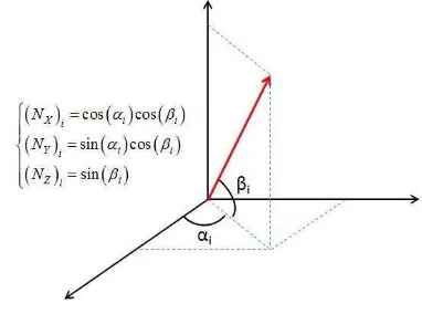
State vector: normals to keep them unitary. Another way to parameterize the system is to express the normals Ni with 2 angles
i, i
. Thefigure 4 displays one possible configuration:
Figure 4: Angle parameterization of the normals
The normals will then be force to be the state vector is then:
The first advantage of this parameterization is to have a simpler formulation than alternative methods using Cartesian coordinates instead of angles (Le Scouarnec, 2013): the constrained problem becomes an unconstrained one. The second advantage is to have a better conditioned system that converges faster.
Solution:
The system is solved iteratively with a weighted non linear least squares algorithm:
0
The solution of this system is well known:
J WJT ΔXJ WT D0 0 HΔX B Where W: Inverse of the observations covariance matrix
Hence, the state vector is updated recursively until a defined
The least squares solution is useful because it provides standard deviations for the estimated parameters. Then the user can refer to these values to evaluate its calibration precision:
diag( xx)
σN1 σNp
The validity of the standard deviations is presented in part 3.
In practice:
The algorithm inputs are:
- LiDAR returns coordinates
LiDAR
LiDARX
- INS orientations {(roll,pitch,heading)}
- The approximate LiDAR-INS configurationCLiDARINS* .
Transforming the INS orientations in a rotation matrix CnINSis straightforward.
Figure 5: Scanning line estimation
On the other hand, the LiDAR returns cannot be used directly. The scanning lines need to be computed. A Principal Component Analysis (PCA) is carried out to estimate the
direction vectoruLiDARi of the i th
scanline in the [LiDAR] frame as shown on Figure 5.
Moreover, the normal vectors need to be approximated in order to accelerate the convergence of the algorithm. They are initialized by the cross product of two randomly chosen direction vectorsˆn
i
u anduˆjn. If these 2 direction vectors belong
to the same plan and are not collinear, we have:
ˆnˆnˆn
estimated yet.N is just an approximate initialization. ˆn
3. RESULTS
3.1 Experimental setups
System configuration
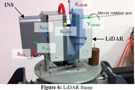
The instruments used are a LiDAR Leica HDS6200 which has a precision lower than 5mm for ranges inferior to 25m and lower than to 1cm for ranges inferior to 50m. The INS is a iXBLUE Landins which provides the attitude with a 0.02° accuracy for the roll and pitch and a 0.1° accuracy for the heading.
The LiDAR system configuration is shown on 6.
Figure 6: LiDAR frame
Definition of the orientations
For simulations and real tests presented in this paper, only 2 plans were used: one vertical and one horizontal (typically the floor or the ceiling). This choice is motivated by practical considerations: most walls scanned in terrestrial laser scanning are horizontal or vertical plans.
The orientation choices are important for a successful calibration. One can show the following scanning orientations are relevant with this system configuration (the demonstration is beyond the scope of this paper):
- Scanning the vertical plan with α angles close to 0°/180°. - Scanning the vertical plan with α angles close to ±70°. The International Archives of the Photogrammetry, Remote Sensing and Spatial Information Sciences, Volume XL-3/W1, 2014
- Scanning the horizontal plan with the LiDAR system tilted with β angles superior to 20° in absolute value.
Figure 7:Vertical plan scanned with an α angle (view from above)
Figure 8: Horizontal plan (floor) scanned with a β angle
3.2 Simulation results
The simulator reproduces the configuration presented in the paragraph dedicated to the system configuration. It is used to generate:
- Random boresight angles.
- p plans with specified orientations. They are chosen roughly vertical or horizontal.
- Noisy INS orientations data (bias and noise) with specified orientations.
- Noisy LiDAR data.
The results presented hereafter are obtained with 2 plans. The 1st plan is approximately vertical (at ±5°) and the 2nd plan is almost horizontal (at ±5°). Each wall is scanned with a given sequence of orientations.
The error distributions are displayed in Figure 10. For the 3 angles, the standard deviation given in Table 8 are inferior to 10-2 degree which was the objective given in the introduction.
0.001° 0.0027° 0.0004°
Table 9: Standard deviations of the boresight angles estimated with the simulated data
Figure 10: Distribution of the boresight errors
(roll/pitch/heading)
Figure 11: Roll/Pitch/Heading normalized residuals
To validate the standard deviations
ˆ ˆ ˆ
,
,
estimated with this procedure, the normalized residuals are calculated.,
: estimated boresight angles,
,
,,
, norm norm norm
: normalized residualsIf the standard deviations are well estimated, then the normal residuals should be distributed according to a standard normal distribution. That means that most normalized residuals (99.7%) should be between -3 and +3 (σnorm=1). The normalized residuals distributions are shown on Figure 11 and prove that the estimated standard deviations are relevant.
3.3 Experimental results
The calibration can be performed on a vehicle, but also directly at the laboratory on a rotating table.
Tests were run in indoor with 2 plans scanned simultaneously: a vertical wall and the floor. The LiDAR scanlines were extracted automatically with a RANSAC algorithm.
The calibration procedure was run several times and estimated parameters are compared in Table 12 and Table 13.
Boresight angles Standard deviations
Roll 0.0588° 0.0104°
Pitch -0.0076° 0.0305°
Heading -0.2754° 0.0323°
Table 12: Results from Test #1
Boresight angles Standard deviations
Roll 0.0469° 0.0098°
Pitch -0.0055° 0.0233°
Heading -0.2965° 0.0304°
Table 13: Results from Test #2
Results from Test#1 and Test#2 show that the differences are coherent with the estimated standard deviations. However, the performances are not as good as the simulation results.
The precision of calibration depends on 2 criteria: the orientation choices and the precision of the scanline vectors u. Since simulations and real data had roughly the same orientations, the performance differences are explained by the u vectors.
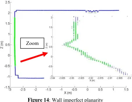
Real data analyses showed that the plans used could have flaws: they are not as ideally planar as simulation plan can be. The
Figure 14 illustrates this imperfect planarity.
Second, the scanlines in the simulator are longer than in the real acquisition. Yet, one can easily understand that the signal to noise ratio decreases as the line becomes longer and u estimation becomes more precise. Additional tests showed that it has a great impact.
Figure 14: Wall imperfect planarity
Therefore, the u vector estimation is the main limitation for this calibration procedure. Before starting a calibration, one should scan entirely the plans considered for the calibration to ensure that they are flat enough. A solution to overcome this limitation would be to use normals instead of scanline vectors because normals estimations are less sensible to the wall local imperfections. These static scans would be performed with a laser settled on a rotating platform.
4. CONCLUSION
In this paper, the boresight calibration problem was tackled with a new approach: a position-free calibration procedure based on orientations. Consequently, calibration does not depend on GPS precision anymore and can even be run directly in the laboratory before setting up the LiDAR system on the vehicle. Simulations proved the efficiency of the method and real datasets confirmed the coherence of the standard deviations. The main limitation of this calibration is the estimation of the u vector. Scanning plans and using their normal is a solution that will be considered in future works.
ACKNOWLEDGEMENTS
This research project is supported by a grant from the Délégation Générale pour l’Armement (DGA).
REFERENCES
Skaloud, J., Litchi, D., 2006, Rigorous approach to boresight self-calibration in airborne laser scanning, ISPRS, Journal of Photogrammetry and Remote Sensing, Vol. 61, Issue 6, pp 414
Skaloud, J.; Schaer, P. Towards automated LiDAR boresight self-calibration. Proceedings of 5th International Symposium on Mobile Mapping Technology, Padova, Italy (29-31 May 2007)
Rieger, P., Studnicka, N., Pfennigbauer, M., Zach, G., 2008. Boresight alignment method for mobile laser scanning systems. Journal of Applied Geodesy. Volume 4, Issue 1, Pages 13–21
Le Scouarnec R., Touzé T., Lacambre J.B., Seube N., 2013, A Positioning free calibration method for mobile laser scanning applications, ISPRS archives – Vol.II-5/W2 2 pp 157-162
iXBlue Landins datasheet.
http://www.ixsea.com/pdf/landins-2011-01-web.pdf Zoom