GRAVITY ANOMALY ASSESSMENT USING GGMS AND AIRBORNE GRAVITY
DATA TOWARDS BATHYMETRY ESTIMATION
A Tugi a, A H M Din a,b*, K M Omar a, A S Mardi a, Z A M Soma, A H Omar a, N A Z Yahaya a, N Yazid a a
Geomatic Innovation Research Group (GIG), Faculty of Geoinformation and Real Estate, Universiti Teknologi Malaysia, 81310 Johor Bahru, Johor, Malaysia.
bGeoscience and Digital Earth Centre (INSTEG), Universiti Teknologi Malaysia, 81310 Johor Bahru, Johor,
Malaysia. *[email protected]
KEY WORDS: Satellite gravity mission, gravity anomaly and Global Geopotential Model.
ABSTRACT:
The Earth’s potential information is important for exploration of the Earth’s gravity field. The techniques of measuring the Earth’s gravity using the terrestrial and ship borne technique are time consuming and have limitation on the vast area. With the space-based measuring technique, these limitations can be overcome. The satellite gravity missions such as Challenging Mini-satellite Payload (CHAMP), Gravity Recovery and Climate Experiment (GRACE), and Gravity-Field and Steady-State Ocean Circulation Explorer Mission (GOCE) has introduced a better way in providing the information on the Earth’s gravity field. From these satellite gravity missions, the Global Geopotential Models (GGMs) has been produced from the spherical harmonics coefficient data type. The information of the gravity anomaly can be used to predict the bathymetry because the gravity anomaly and bathymetry have relationships between each other. There are many GGMs that have been published and each of the models gives a different value of the Earth’s gravity field information. Therefore, this study is conducted to assess the most reliable GGM for the Malaysian Seas. This study covered the area of the marine area on the South China Sea at Sabah extent. Seven GGMs have been selected from the three satellite gravity missions. The gravity anomalies derived from the GGMs are compared with the airborne gravity anomaly, in order to figure out the correlation (R2) and the root mean square error (RMSE) of the data. From these assessments, the most suitable GGMs for the study area is GOCE model, GO_CONS_GCF_2_TIMR4 with the R2 and RMSE value of 0.7899 and 9.886 mGal, respectively. This selected model will be used in the estimating the bathymetry for Malaysian Seas in future.
1. BASIC PRINCIPLES AND THEORY
1.1 Introduction
The advancement of the technologies in determining the Earth’s gravity field has contributed to the broad exploration of the quality of the recent global gravity field. Space-based technique is able to provide a better result in terms of coverage and reasonable time. Furthermore, the Earth’s gravity field can be explored at scales down to hundreds and thousands of kilometres. Nevertheless, this technique has some limitations in retrieving gravity field due to the low sensitivity of the high degree geopotential spherical harmonic coefficient caused by a strong signal attenuation with altitude (Heiskanen & Moritz, 1967; Karpik et al., 2016). The deliverable of the satellite gravimetric missions is the Global Geopotential Model (GGM). Based on the information from GGM, the gravity anomaly, geoid height and the deflections of vertical can be derived. The data derived by the GGM can provide a better long and medium wavelength part of the gravimetric geoid in terms of the quality of data which is accuracy and resolution (Sadiq & Ahmad, 2009). There are many GGM published by the International Centre of Global Earth Models (ICGEM) and to test the quality of the Earth’s potential information derived from the models, a study need to be conducted. This study will help to evaluate the most compatible global model from the other
models and these global models will fit differently according to the area of interest. According to the study conducted by Featherstone (1998) and Sadiq & Ahmad (2009), the GGM evaluation are being conducted to help in establishing the best fit localize global model for their region. In this study, the evaluation of the GGM being piloted in order to test the most suitable global model as an input data towards the bathymetry estimation for the Malaysian Seas from the gravity anomaly data around the water area.
1.2 Satellite Gravity Mission
technique. However, according to Xu et al. (2007), these techniques have some limitations in terms of the distribution of the data and data inconsistencies. Therefore, the advancement of the space-borne technique are likely being chosen for the Earth’s gravity measurement technique because it can give a global, regular and dense gravity data coverage with high and homogeneous quality.
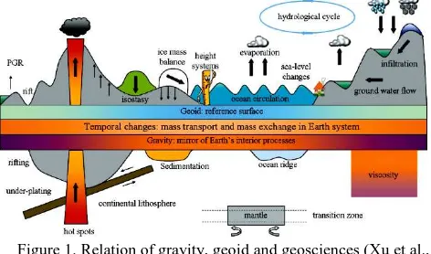
Figure 1. Relation of gravity, geoid and geosciences (Xu et al., 2007)
The measurements of the Earth’s gravity from space-borne technique are divided into three different ideas. The first idea or concept of the space-borne gravimetry is satellite-to-satellite tracking in high-low mode (SST-hl). A low Earth orbiter (LEO) is attracted to the mass anomalies while flying at a few hundred kilometres of altitude and its precise position and velocities are tracked and defined by the Global Positioning System (GPS). The space-borne satellite that implements this concept was the German geo-specific mission, which is Challenging Minisatellite Payload (CHAMP). However, the gravity of the Earth cannot be measured directly from the space-borne technique. The measurement needs to be derived from the direct observables of the continuous tracking and the accelerometer data. Figure 2 shows the concept of the SST-hl.
The second concept of space-borne gravimetric measurement is the satellite-to-satellite tracking in low mode (SST-ll) (see Figure 3). Two LEO satellites with a distance of hundred kilometres between each other are placed in the same orbit and the relative motion the two satellites is measured by the inter-satellite K-band ranging system with a high accuracies (ESA, 1999; Xu et al., 2007). The satellite gravity mission that implemented this concept is Gravity Recovery and Climate Experiment (GRACE) mission.
Figure 2. Concept of satellite-to-satellite tracking in the high-low mode (SST-hl) (ESA, 1999).
Lastly, the third idea of the gravity measurement is the satellite gravity gradiometry (SGG). This system includes three pairs of accelerometers that are highly sensitive in a diamond configuration that is located close to the mass centre. The SGG observes the second derivatives of the gravitational potential, meanwhile for the geo-locating gravity field and the observation from gradiometer will be determined by GPS satellite-to-satellite tracking (SST) measurement (Schall et. al, 2014). Moreover, on each of the instrument triad, two accelerometers are placed. Satellite of Gravity-Field and Steady-State Ocean Circulation Explorer Mission (GOCE) implement this concept. Figure 4 illustrates the concept of SGG. This is dedicated to measure the Earth’ static gravity field and to model the geoid that can provide a high accuracy and spatial resolution, which is 1 cm accuracy over 100km expected (Xu et al., 2007).
Figure 3. Concept of satellite-to-satellite tracking in the low-low mode (SST-ll) (ESA, 1999).
Figure 4. Concept of satellite gravity gradiometry (SGG) (ESA, 1999).
1.3 Global Geopotential Models
For the tailored GGM, the information of the measurement is derived from the refining the existing satellite-only or the combined GGM using the local or regional gravity and topography data. The GGM data of spherical harmonic coefficient is a public domain that is published by the International Centre of Global Earth Models (ICGEM) (Sprlak
et al., 2011). In ICGEM website
(http://icgem.gfz-potsdam.de/ICGEM/), published by the which are the satellite-only model and combined model. Satellite-satellite-only model consists of only satellite-based gravity observation, such as from CHAMP, GRACE, and GOCE) or combined together with other satellite missions such as Laser Geodynamic Satellite (LAGEOS). The information about the satellite involved in the observation of the GGM can be obtained from the GGM file header.
The GGM data provides by the ICGEM is the spherical harmonic coefficient data comprises of a fully normalized Stokes’ coefficient for the degree (n) and order (m) ( and
) and its respective standard errors (σ and ), Newtonian gravitational constants (G) and the mass of the Earth (M), normal gravity on the surface of the reference ellipsoid (γ) and reference radius (r) (Heiskanen & Moritz, 1967; Erol et al., 2009; Sulaiman, 2016). From the provided data, the computation of the gravity anomaly and the geoid undulation with the deflections of vertical can be done. The formulas of the computation are expressed in Equation (1) and (2).
(-1) +
GM : Product of the Earth’s mass and the gravitational constant
R : radial distance of the computation point / : Normalized harmonic coefficients
: Normalized Legendre function
θ and γ : Geodetic latitude and longitude of the computation point
The GGM model might have a different spherical harmonic coefficient and this influence the resolution of the gravity anomaly and geoid heights derived from GGM because the resolution is determined according to the maximum number of complete spherical harmonic expansions (max). Besides that, the uses of the space-borne technique in measuring the Earth’s gravity are reliable and dependable. A study on the Earth’s gravity has been conducted by Einarsson et al. (2010) on the gravity changes due to the Sumatra-Andaman and Nias earthquakes using GRACE satellite mission. GRACE data were used to recover the gravity field of the earth up to spherical harmonic degree 120.
1.4 Gravity Anomaly Definition and Concept
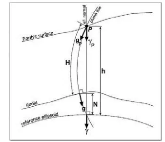
From the Earth’s geopotential derived from GGMs, gravity anomaly is one of the information that is provided. Gravity anomaly can be defined as a difference of the gravitational acceleration due to the Earth masses and the gravitational acceleration generated by some reference mass distribution (Hackney & Featherstone, 2003). This gravity anomaly is important and essential in geodesy and geophysics field. The gravity anomaly can be used in determining the shape of the Earth, represented by geoid, which is the equipotential surface of the Earth‘s gravity field that approximately resemble the mean sea level surface. In addition, gravity anomaly can be used in the realization of the variation in mass-density and the geological structure of the Earth’s subsurface for a wide range of application (Hackney & Featherstone, 2003). In geodesy, the reference surface is refer to geoid but for geophysics, the focus is on the relative difference of the gravity and the reference level can be chosen from the arbitrary height such as the elevation mean of the selected area. Figure 5 illustrates the parameters used in defining the gravity anomalies and gravity disturbance where g is the gravity vector at the geoid, while γ is the normal gravity vector at the surface of the ellipsoid. Furthermore, gP is
the vector quantity of gravity and γP is the magnitude of normal
gravity, both at point P (in this case, the Earth’s topography surface) and H is the orthometric height along the curved plumb line. N is the geoid–ellipsoid separation and h is ellipsoidal height along the ellipsoidal surface normal.
Figure 5. Parameters used to define gravity anomalies and gravity disturbances (Hackney & Featherstone, 2003) 1.5 Relationship between Gravity Anomaly and Depth
Figure 6. Topography on the ocean floor adds its own attraction to Earth’s usual gravity (Smith and Sandwell, 2004)
2. RESEARCH APPROACH
2.1 Study Area
In this study, the area that is focused on is at the East Malaysia which cover the South China Sea in Sabah extent with the latitude range between 3° 04’ 00”E until 9° 00’ 00” E and longitude range between 110° 43’ N until 119° 30’ N. Figure 7 shows the coverage of the study area for the assessment of GGM gravity anomaly (in the red box). This study is focusing on the gravity anomaly at the water area or the marine territory.
Figure 7. Study area 2.2 Data Analysis and Methodology
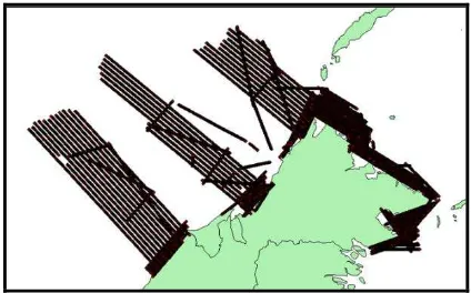
The data that are used for the gravity anomaly evaluation are the GGM data from the International Centre for Global Earth Models (ICGEM), the airborne gravity anomaly data from Department of Survey and Mapping Malaysia (DSMM) and single beam bathymetry data from the National Hydrographic Centre (NHC). Figure 8 depicts the gravity anomaly track from airborne survey that is conducted by DSMM for the year 2015 along the South China Sea, meanwhile Figure 9 display the single-beam bathymetry survey area that is piloted by NHC.
Figure 8. Airborne track of gravity anomaly
Figure 9. Single beam bathymetry survey.
The airborne gravity anomaly data from DSMM are used to assess the best gravity anomaly from GGM. The airborne data is used because it can provide a better accuracy compare to the space-based technique. However, space-based technique can provide an enormous data coverage and even though it provides solutions with less resolution than terrestrial and airborne gravimetric methods, the data from satellite gravity mission can significantly contribute in obtaining a precise determination and better information about the medium and long wavelengths of the gravity field and its temporal variations (Sadiq et. al, 2010).
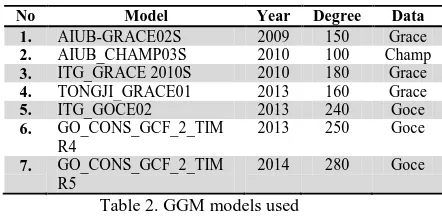
The result that was obtained from this study is to examine the most suitable gravity anomaly model for Malaysia region. The main satellite gravity missions used are Challenging Mini-satellite Payload (CHAMP), Gravity Recovery and Climate Experiment (GRACE) and Gravity Field and Steady-State Ocean Circulation Explorer (GOCE). Table 1 listed the Satellite Gravity Missions that were used (summarised from ESA, NASA & GFZ Potsdam, 2016).
Table.1 Satellite Gravity Missions used
2.3 Data Processing
The assessment of the GGM being piloted by randomly choose 130 points from each data which is from GGM and airborne gravity anomaly in order to compare the gravity anomaly value for each of the selected points. In deriving the spherical harmonic coefficient from GGM, Matlab software was used with the coding made by Mehdi Eshagh and Ramin Kiamehr (2012) from Divison of Geodesy, Royal Institute of Technology, Stockholm, Sweden.
As for the assessment of the GGM, it was conducted by analysing the root mean square error (RMSE) between the GGM gravity anomaly data and the airborne data. This RMSE or the root mean square deviation (RMSD) is the analysis used to measure the difference between the observed values and the values from of predicted model. From this analysis, the difference between the two different data is called residual of the error; meanwhile the RMSE is the value to accumulate the residuals into a single predictive power measurement. The formula of RMSE that applied is shown in the Equation (3) and (4).
Residual = Xobs – Xmodel (3)
RMSE
=
(4)
Table 2. GGM models used
In this case, the value of Xobs is the GGM gravity anomaly data, while Xmodel is the airborne gravity anomaly data, n representing
the total of the data used. Moreover, the correlation between both of the gravity information is discussed in order to justify the most suitable model that will be used for further study.
3. RESULTS AND DISCUSSIONS
3.1 Gravity Anomaly Map from GGM Models
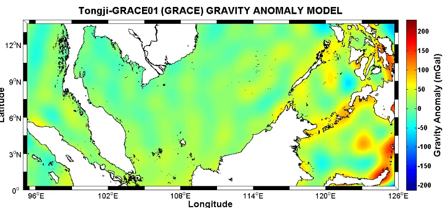
In this section, all of the seven selected GGM were mapped by using the Matlab software in order to depict the undulation or the trend of the gravity anomaly for Malaysian Seas. Figure 10 to 12 shows the gravity anomaly map for AIUB_CHAMP03S, ITG-Grace2010s and AIUB-GRACE02S, respectively. Furthermore, Figure 13 to 16 illustrates the gravity anomaly for a GGM model of Tongji-GRACE01, ITG-Goce02, GO_CONS_GCF_2_TIM_R4 and GO_CONS_GCF_2_TIM R5 correspondingly.
Figure 10. AIUB_CHAMPS03 gravity anomaly model
No Model Year Degree Data
1. AIUB-GRACE02S 2009 150 Grace
2. AIUB_CHAMP03S 2010 100 Champ
3. ITG_GRACE 2010S 2010 180 Grace
4. TONGJI_GRACE01 2013 160 Grace
5. ITG_GOCE02 2013 240 Goce
6. GO_CONS_GCF_2_TIM
R4
2013 250 Goce
7. GO_CONS_GCF_2_TIM
R5
Figure 11. ITG-Grace2010s gravity anomaly model
Figure 12. AIUB-GRACE02S gravity anomaly model
Figure 14. ITG-Goce02 gravity anomaly model
Figure 15. GO_CONS_GCF_2_TIMR4 gravity anomaly model
Based on the colour scale of the map from Figure 10 to 16, it can be explained that most of the gravity anomaly models are range from +50mGal to -50mGal. The difference in the negative and the positive values indicates the position of the gravity anomaly from its reference surface which is ellipsoid. The 0 mGal gravity anomaly is assumed as the ellipsoid surface. Therefore, the positive gravity anomaly value denotes that the gravity anomaly is above the ellipsoid surface, meanwhile the negative gravity anomaly represents the value that is below the ellipsoid surface.
3.2 Combination of the Gravity Anomaly from Airborne and GGM
The 130 selected points for the validation between the gravity anomaly from airborne and GGM is plotted on a graph to show the pattern and the corresponding relationship between them. Figure 17 shows the graph of the gravity anomaly combination between airborne and the selected GGM.
From the graph shown in Figure 17, the gravity anomaly model that has a similar and closely resembles the pattern of airborne gravity anomaly is the model from GOCE satellite mission which is GO_CONS_GCF_2_TIMR4. Furthermore, from Figure 17, the models that show the nearly pattern of the airborne gravity is the models from the GOCE satellite mission which is GO_CONS_GCF_2_TIMR5, and ITG Goce02.
Figure 17. Graph of the combination of gravity anomaly from airborne and GGMs
3.3 Correlation between the airborne gravity anomaly and GGM
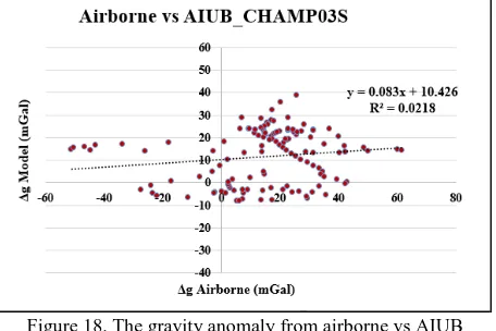
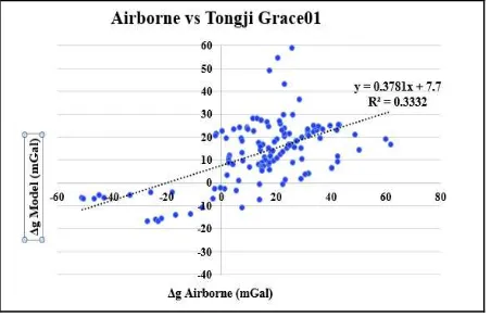
According to the graph shown in Figure 17, the model that has the most similar pattern with the airborne gravity anomaly variation is GO_CONS_GCF_2_TIMR4. In order to make the decision on determining the appropriate GGM to be used for further investigation, the correlation (R2) between airborne and GGM is being conducted. The correlation between airborne gravity data and GGM are computed using Microsoft Excel. The x-axis of the graph is the gravity anomaly from airborne, while the y-axis is the gravity anomaly derived from GGM. Figure 18 to 24 shows the graph of the distribution 130 points of validation and the R2 between each of the GGM and airborne gravity anomaly value for AIUB_CHAMP03S, ITG Grace2010s, Tongji-Grace01, AIUB Grace02S, ITG Goce02, GO_CONS_GCF_2_TIMR4 and GO_CONS_GCF_2_TIM R5, respectively.
From the correlation analysis, it shows that the GO_CONS_GCF_2_ TIMR4 has the highest value of R2 when it is compared with the other models with 0.7899. The GO_CONS_GCF_2_ TIMR5 is the second model that has a better correlation after GO_CONS_GCF_2_ TIMR4 with 0.7729. The model that has the poorest R2 is AIUB_CHAMP03S with 0.0218. This condition indicates that AIUB_CHAMP03S gravity anomaly is not a good model to be used for further analysis in this study area. The R2 value of the other models is being discussed in the next section (Section 3.4).
Figure 18. The gravity anomaly from airborne vs AIUB CHAMP03S
Figure 20. The gravity anomaly from airborne vs Tongji Grace01
Figure 21. The gravity anomaly from airborne vs AIUB Grace02S
Figure 22. The gravity anomaly from airborne vs ITG Goce02
Figure 23. The gravity anomaly from airborne vs GO_CONS_GCF_2_TIMR4
Figure 24. The gravity anomaly from airborne vs GO_CONS_GCF_2_TIMR5
3.4 Statistical analysis between the airborne data and GGM gravity anomaly
This section discussed in the statistical analysis of the gravity anomaly values for each model in terms of its minimum and maximum difference between the airborne data and GGMs, the mean of the different, RMSE and the R2 of the gravity anomaly. From these analyses, the most reliable and well-fit model for this study area can be determined. Table 3 shows the statistical values of each of the GGM.
From Table 3, it can be seen that the GO_CONS _GCF_2_TIMR4 shows the lowest RMSE and standard error value with 9.886 and 9.634 in mGal units, respectively. The lower value of the RMSE indicates that the gravity anomaly different between the airborne and the GGM is small. Even though the degree and order of the GO_CONS _GCF_2_TIMR4 is not the highest among the seven selected models, it still provides a better statistical value compared to the GO_CONS _GCF_2_TIMR5, which has the highest number of degree and order. The RMSE different between the airborne and GGM gravity anomaly is influenced by the accuracy of the data. All of the GGM gravity anomaly data are obtained from satellite gravity mission which have long wavelength meanwhile the airborne gravity anomaly data have medium or short wavelength.
Moreover, the correlation analysis between the airborne and the GGMs shows that the GO_CONS _GCF_2_TIMR4 has the highest value which is 0.7899, compared to the other models. A good correlation value between two sets of data will practically be nearest to 1. Moreover, from this statistical analysis, it shows that the other models from GOCE satellite gravity mission gives more reliable values compared to the GRACE models and CHAMP model.
Therefore, it can be concluded that the model that is reliable for this study area belongs to GGM under the GOCE satellite gravity mission, followed by GGM from GRACE satellite
gravity mission, and last but not least, the GGM from CHAMP mission.
Table 3. Statistical analysis of the gravity anomaly for the selected GGM 3.5 Pattern between Gravity Anomaly and Bathymetry
data
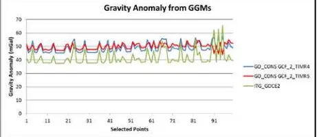
After the selection of the most reliable and the most suitable GGM has accomplished, the GO_CONS _GCF_2_TIMR4 model will be used in estimating the bathymetry for Malaysian Seas. In this section, only the pattern of the gravity anomaly from the best three selected models and the bathymetry data obtained from NHC will be discussed. The relationship of the gravity anomaly and gravity data can be seen through the pattern of the data. A number of 100 different points were randomly chosen for this assessment, to illustrate the relationship between these data. Figure 25 illustrates the pattern of the gravity anomaly from GO_CONS GCF_2_TIMR4, GO_CONS GCF_2_TIMR5 and ITG_GOCE2 and Figure 26 shows the pattern of the bathymetry data from NHC.illustrates the pattern of the gravity anomaly from GO_CONS GCF_2_TIMR4 and Figure 26 shows the pattern of the bathymetry data from the NHC.
Figure 25. The pattern of 100 selected points of TIM_R4, TIMR5 and ITG_GOCE2 derived-gravity anomaly data
Figure 26. The pattern of 100 selected points of the single beam bathymetry data
Based on the Figure 25 and 26, the pattern of the gravity anomaly and the bathymetry data show the similar fluctuation between each other. Even though the gravity anomaly values between the three selected GGMs, the pattern of the gravity
anomaly for 100 selected points shows the similarities between the models. Therefore, this result summarised that the gravity anomaly and bathymetry data have connection between each other and this is supported by the study made by Smith & Sandwell (2004). However, according to Smith (1997) and Jena (2012), the bathymetry or gravity ratio varies spatially because of the sediment thickness difference and other geological factors, and this will make the bathymetry estimation is a complex process.
4. CONCLUSION
With the realization of the GGMs, the gathering of the Earth’s potential information becomes easier and reliable. Moreover, the number of degree and order of the spherical harmonic coefficient influences the accuracy and the resolution of the GGM. This study demonstrated that the model of GOCE satellite mission provides better and more reliable information on the gravity anomaly when compared to another model from CHAMP and GRACE satellite missions. The compatibility of the GGM is connected to the area or the region of the study. Different GGM might be reliable in the different area. Therefore, for this study area, the most reliable GGM is the model of GOCE satellite mission, namely GO_CONS _GCF_2_TIMR4.
ACKNOWLEDGEMENTS
REFERENCES
Einarsson, I., Hoechner, A., Wang, R., & Kusche, J., 2010. Gravity changes due to the Sumatra-Andaman and Nias earthquakes as detected by the GRACE satellites: A reexamination. Geophysical Journal International, 183(2), 733– 747. http://doi.org/10.1111/j.1365-246X.2010.04756.x
Erol, B., Sideris, M. G., Celik, R. N., 2009. Comparison of global geopotential models from the champ and grace missions for regional geoid modelling in Turkey. Studia Geophysica et Geodaetica, 53(4), 419–441. http://doi.org/10.1007/s11200-009-0032-8
ESA, 1999. Gravity Field and Steady-State Ocean Circulation Mission, Report for mission selection of the four candidate Earth Explorer missions. Esa Sp, 1233(1).
Featherstone, W. E., 1998. Comparison of Different Satellite Altimeter-Derived Gravity Anomaly Grids with Ship-Borne Gravity Data around Australia. Differences, 1–6.
Hackney, R. I., & Featherstone, W. E. (2003). Geodetic versus geophysical perspectives of the “gravity anomaly.” Geophysical Journal International, 154(1), 35–43. http://doi.org/10.1046/j.1365-246X.2003.01941.x
Jena, B., Kurian, P. J., Swain, D., Tyagi, A., & Ravindra, R. (2012). Prediction of bathymetry from satellite altimeter based gravity in the arabian sea: Mapping of two unnamed deep seamounts. International Journal of Applied Earth Observation
and Geoinformation, 16(1), 1–4. http://doi.org/10.1016/j.
jag.2011.11.008
Karpik, A. P., Kanushin, V. F., Ganagina, I. G., Goldobin, D. N., Kosarev, N. S., & Kosareva, A. M. (2016). Evaluation of recent Earth’s global gravity field models with terrestrial gravity data. Contributions to Geophysics and Geodesy, 46(1), 1–11. http://doi.org/10.1515/congeo-2016-0001
Kearsley, A. H. W., & Forsberg, R. (1990). Tailored Geopotential Models - applications and shortcomings. Manuscripta Geodetica, 15(July), 151–158.
Sadiq, M., & Ahmad, Z. (2009). On the selection of optimal global geopotential model for geoid modeling: A case study in Pakistan. Advances in Space Research, 44(5), 627–639. http://doi.org/10.1016/j.asr.2009.05.004
Sadiq, M., Tscherning, C. C., & Ahmad, Z. (2010). Regional gravity field model in Pakistan area from the combination of CHAMP, GRACE, and ground data using least squares collocation: A case study. Advances in Space Research 46. Schall, J., Eicker, A., & Kusche, J. (2014). The ITG-Goce02 gravity field model from GOCE orbit and gradiometer data based on the short arc approach. Institute of Geodesy and Geoinformation, Bonn University: Springer-Verlag Berlin Heidelberg.
Smith, W. H. (1997). Global Sea Floor Topography from Satellite Altimetry and Ship Depth Soundings. Science, 277 (5334), 1956–1962. http://doi.org/10.1126/science.277.5334. 1956
Smith, W., & Sandwell, D. (2004). Conventional Bathymetry, Bathymetry from Space, and Geodetic Altimetry. Oceanography, 17(1), 8–23. http://doi.org/10.5670/oceanog. 2004.63
Sprlak, M., Gerlach, C., Omang, O. C., & Pettersen, B. R. (2011). Comparison of GOCE derived satellite global gravity models with EGM2008, the OCTAS Geoid and terrestrial gravity data: Case study for Norway. Proc. of ‘4th International
GOCE User Workshop’. Munich, Germany.