An equation for irregular distributions of leaf azimuth density
C.B.S. Teh
a,∗, L.P. Simmonds
a, T.R. Wheeler
baDepartment of Soil Science, University of Reading, Whiteknights, P.O. Box 233, Reading RG6 6DW, UK bDepartment of Agriculture, University of Reading, Earley Gate, P.O. Box 236, Reading RG6 2AT, UK
Received 5 August 1999; received in revised form 21 February 2000; accepted 29 February 2000
Abstract
The von Mises equation was modified to describe numerically irregular distributions of leaf azimuth density. The new equation has three indexes: T (describing distribution elongation), S (describing number of azimuth preferences), and R (describing general canopy azimuth position). The equation was tested on two contrasting canopies: sunflower and maize. In 1998, the diurnal variation of leaf azimuths was measured weekly beginning 66 days after planting for 5 weeks. The equation was tested again in 1999. The equation characterised the leaf azimuth densities accurately (mean absolute estimation error of 0.05). For sunflower, R index was linearly related to sun azimuth, and sunflower generally tracked the sun in the same way for both years because they had almost equal R at a given sun azimuth. However, the azimuth density distribution in 1999 was slightly more clumped than in 1998, and that sunflower canopies in 1998 would fluctuate between one to two azimuth preferences, but sunflower in 1999 generally showed one azimuth preference. For maize, mean T, S and R for 1998 and 1999 were similar to each other. These values agreed with field observations, where maize canopies were usually elongated, having two azimuth preferences that were perpendicular to planting row direction. Logistic regression showed that these indexes were descriptive enough to differentiate between sunflower and maize canopies with an accuracy greater than 80%. The most important index to differentiate between canopy types was T, S, then R. © 2000 Elsevier Science B.V. All rights reserved.
Keywords: Leaf azimuth; Canopy architecture; von Mises; Radiation model
1. Introduction
Canopy architecture describes how a canopy occu-pies the aerial space and is a major factor influencing how much radiation a given leaf area index will in-tercept. Canopy architecture is often characterised by the density distributions of leaf inclination (leaf angle from vertical) and leaf azimuth (leaf angle from north in a clockwise direction). The density distribution of leaf inclination and azimuth correspond to the
proba-∗Corresponding author. Tel.:+44-118-931-6557;
fax:+44-118-931-6666.
E-mail address: [email protected] (C.B.S. Teh)
bility of finding a leaf in a particular inclination and azimuth range, respectively (Lemeur, 1973a).
The distribution of leaf inclination density can be divided into four groups: planophile, erec-tophile, plagiophile and extremophile (de Wit, 1965). Planophile and erectophile canopies are dominated by horizontally-inclined and vertically-inclined leaves, respectively. Sunflower is a crop with a planophile canopy, whereas most grass species have erectophile canopies. In contrast, the leaf arrangement of plagio-phile canopies like maize are predominantly about
45◦. Extremophile canopies are rare because their
leaf arrangements are predominantly both horizontal and vertical with very few leaves arranged within the intermediate inclination range. Equations to describe
these four leaf inclination groups have been developed by de Wit (1965), and Lemeur (1973a).
Work on characterising leaf azimuth densities, how-ever, is rarer. One equation to characterise the distribu-tion of leaf azimuth density g(φ) was given by Lemeur (1973a)
g(φ)= a
2b2
a2sin2φ+b2cos2φ (1)
where g(φ) describes the probability of a leaf within azimuth range (φ,φ+δφ). Eq. (1) assumes the canopy azimuth is an ellipsoid with a centre at the origin and with semi-axis lengths a and b. The use of this equation is limited because, as noted by Lemeur himself, the variety of distributional shapes that can be simulated using Eq. (1) is very limited. More-over, because the distribution is centred at the origin, Eq. (1) cannot be used to characterise heliotropic (solar-tracking) canopies like sunflower and cotton. Heliotropic canopies that follow the sun’s movement will tend to lean or point towards the sun. These movements will move the centre of distribution of leaf azimuth density away from the origin.
Shell et al. (1974), and Shell and Lang (1975, 1976) used the von Mises’s density function to characterise leaf azimuth density. This equation is given by
g(φ)= 1
2π I0(κ)
exp{κcos(φ−u0)} (2)
where u0 is the mean direction, κ the concentration
parameter and I0(κ) is the modified Bessel function
of the first kind and order zero. Eq. (2) is more useful than Eq. (1) because varying the values of u0 andκ
will yield a greater variety of distributional shapes and better characterisation of canopy heliotropism. Despite its advantages over Eqs. (1) and (2) may still fail to characterise the observed distributions closely, especially if the distribution of leaf azimuth density is irregular or show more than a single azimuth prefer-ence. Maize canopies, for example, are well-known to have two azimuth preferences that are perpendicular to the planting row direction (Loomis and Williams, 1969; Lemeur, 1973b).
The purpose of this study was: (1) to develop an equation that could characterise a wide range of leaf azimuth densities more accurately, especially for canopies with irregular azimuth distributions,
and (2) to use the new equation to describe numer-ically the leaf azimuth density of two contrasting canopy types: a heliotropic canopy (sunflower), and a non-heliotropic canopy (maize). This new equation does not aim to be predictive; that is, it is not to predict the leaf azimuth density without any canopy architecture measurements. Rather, the equation aims to be descriptive; that is, to describe numerically the azimuth density distribution. The advantages of having numerical descriptions are that one can more easily compare any changes in azimuth distribution of a crop species between growing seasons, between crop treatments, or between crop varieties. Without numerical descriptions, any comparisons between leaf azimuth densities must be done visually by graphs. In short, the new equation was developed to provide a quantitative description of leaf azimuth density, as well as a quantitative measure of canopy azimuth differences. Though this equation was not meant to be predictive, this paper will describe experiments conducted in two growing seasons to test whether the equation’s parameters determined for one crop in one season was similar to the parameters determined in a different season. This could indicate promise whether the equation could predict the canopy azimuth density for a given cultivar of a crop species.
2. Leaf azimuth density equation
Eq. (2) was modified to
g(φ)= 1
2π I0(T )
exp{Tcos[S(R−φ)+d(φ)]} (3)
where T is called the thickness or elongation index (dimensionless); S the shape (or number of azimuth preferences) index (dimensionless); R the rotation (or general canopy azimuth position) index (degrees or radians); and d(φ) is a distortion distribution, given by:
d(φ)=cos[S(R−φ)]. Note that T and R in Eq. (3)
are synonymous toκ and u0 in Eq. (2), respectively.
The parameter names in Eq. (3) were chosen so they better reflect their purpose and usage in the context of canopy architecture description.
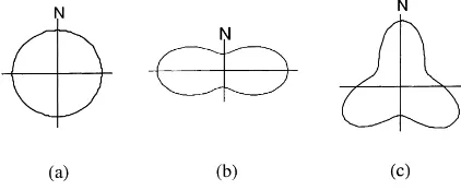
Fig. 1. Polar graphs showing various distributions of leaf azimuth density generated using Eq. (3) with distortion distribution d(φ)=0 (N indicates north). (a) T=0.00, S=1, R=0◦; (b) T=0.70, S=2,
R=90◦; (c) T=0.40, S=3, R=0◦ (note: T, S and R are thickness,
shape and rotation index, respectively).
of T will increase the distribution stretch or elonga-tion. The S index indicates the number of azimuth preferences, and this gives the distribution a distinct shape. When S=0 or 1, for example, the distribution shape is a circle (no azimuth preference); S=2 pro-duces a distribution with two azimuth preferences so the distribution looks like a ‘8’ or a stretched cir-cle; and S=3 produces three azimuth preferences so the distribution looks like three apices. The R index indicates the general canopy azimuth position, and varying its value rotates the distribution around the origin, where positive R rotates the distribution clock-wise. This rotation index is crucial in the characteri-sation of canopy heliotropism because R can be used
to describe canopy movement (Fig. 2 ). When S=1,
for example, varying the thickness index T can shift the centre of distribution to describe the canopy lean-ing or pointlean-ing toward a specific direction such as to-wards the sun. Greater values of T will shift the canopy even more. The rotation index R can then be used to characterise the movement or solar-tracking by the canopy.
Fig. 2. Simulation of a heliotropic canopy with T=0.55, S=1, and distortion distribution d(φ)=0. The canopy tracks the sun movement from (a) to (d) (N indicates north; arrow indicates the sun’s azimuth). (a) R=90◦ when sun is at east; (b) R=135◦when sun is at south-east; (c)
R=225◦when sun is at south-west; (d) R=270◦when sun is at west (note: T, S and R are thickness, shape and rotation index, respectively).
Fig. 1a is the distribution of a perfectly random leaf azimuth density. For this distribution, the canopy has no preferential azimuth direction, and this distribution is usually assumed by workers when canopy azimuth is unknown or not measured. Fig. 1b is a typical dis-tribution for maize canopies where their leaves tend to be orientated perpendicularly to the planting row di-rection. Sunflower has been shown to have a distribu-tion like in Fig. 1c (Lemeur, 1973b), where its leaves tend to be separated about 120◦from each other (i.e.
three azimuth preferences).
The distortion distribution d(φ) (that includes a S index as well) is an attempt to distort the distribu-tion in a controlled manner. Canopies in reality may not be distributed so regularly or smoothly as shown in Figs. 1 and 2. From Eq. (3), the term S(R−φ) in cos[S(R−φ)+d(φ)] is altered by a non-constant value taken from another cosine distribution described by
d(φ). Consequently, the exponential function in Eq. (3) is dependent on two cosine distributions, where
d(φ) acts to further alter (or ‘distort’) the term in the exponential function. From our experience, Eq. (3) is well-behaved when values of the indexes T, S, and
R are restricted in the range of 0.0–2.0, 0.0–3.0, and
0–300◦, respectively.
Since Eq. (3) characterises the spatial distribution of leaf azimuth, this equation could also be used in some detailed plant radiation models (e.g., the G-function in Ross and Nilson, 1966; Fukai and Loomis, 1976) to determine the radiant flux density within canopies. Nevertheless, it is difficult to integrate Eq. (3) analyt-ically; hence, integration must be done numerically (which can be done using most mathematical soft-ware). Eq. (3) should be normalised to unity over
the range (0–360◦) before one wishes to determine
(φ,φ+δφ), or before using Eq. (3) in plant radiation models.
3. Materials and methods
The usefulness of Eq. (3) was tested on two crops with differing canopy types: sunflower (Helianthus
an-nuus L. hybrid Sanluca) and maize (Zea mays L.
hy-brid Hudson). These two crops were planted on 22 May 1998 at Sonning Farm (51◦27′N; 0◦58′W). Field size was approximately 0.13 ha and planting rows were in the NE–SW direction. Planting density for each crop was 60,000 plants ha−1, and row spacing was 0.6 m. No irrigation was supplied throughout the growing season; the crops were rain-fed.
Canopy architecture measurements on maize and sunflower started 66 days after planting (27 July 1998), and continued every week for 5 weeks. For each data collection period, leaf azimuths of three sunflower plants and three maize plants were measured using a compass for 4–6 periods in a day. Canopy measure-ments usually begun at 10:00 hours and ended at 17:00 hours. In addition, leaf areas were measured using a leaf area machine (LI-COR, Lincoln, NE, USA; Model 3000).
The method described by Lemeur (1973b) was used to determine the leaf azimuth density. Leaf azimuths were categorised into eight classes of 45◦ intervals: 337.5–22.5, 22.5–67.5,. . ., 292.5–337.5◦. For each leaf azimuth class, the area of all leaves were pooled (summed), and the pooled area was divided by the total leaf area for all azimuth classes. Finally, division by π/4 (45◦) yielded the density for a leaf azimuth
class. This division was necessary so that integration of the leaf azimuth density over the range (0–360◦) is unity.
Eq. (3) was then fitted to the observed leaf azimuth densities. The indices T, S, and R were estimated by minimising the error sum of squares between observed and simulated densities. The error sum of squares was minimised using Microsoft Excel® Solver Version 8.0 (Microsoft Corp., Redmond, Washington, USA), which uses a non-linear optimisation algorithm called Generalized Reduced Gradient (Lasdon et al., 1978). The average error of estimation was calculated us-ing the statistic absolute mean error (AME) that com-pares n pairs of measured (M) and simulated (S) values
as
The same field experiment was repeated in the sec-ond year to test the fit of Eq. (3) against another data set of maize and sunflower. The second field experi-ment was exactly the same as the first except planting date was 5 May 1999, and field size was approximately 0.07 ha. The same canopy architecture measurements on maize and sunflower started 56 days after plant-ing (30 June 1999), and continued every week for two weeks. Leaf area and azimuth data were treated and analysed in the same way as described previously.
As an alternative way to observe the heliotropism of sunflower, the angle between the leaf normal and sun direction was calculated. This angle indicates how the sunflower leaf faces the sun. When the angle is 0◦, the leaf is at maximum exposure to the sun. Conversely, a 90◦angle indicates the leaf is at minimum exposure. This angleγ was calculated by
γ=arccos[cosθcosθL+sinθsinθLcos(φ−φL)] (4)
where θ is the sun inclination, θL the leaf
inclina-tion, φ the sun azimuth and φL is the leaf azimuth
(Ross, 1981). The various angles between the sun-flower leaves and sun direction were classified into six classes of 15◦ intervals: 0–15◦, 15–30◦,. . ., 75–90◦. The distribution ofγ was then expressed as the frac-tion of leaf area belonging in a particularγ class to the total leaf area.
Lastly, logistic regression was used to determine how well the three leaf azimuth indexes (T, S, and
R) could be used to discriminate between sunflower
and maize canopies. Discriminant analysis could also be used but this analysis requires more restrictive as-sumptions than those for logistic regression. Logistic regression analysis was by SPSS® Version 7.0 (SPSS Inc., Chicago, IL, USA). Before analysis, sunflower classification was coded as 0, and maize as 1.
4. Results and discussion
4.1. Leaf azimuth density of sunflower
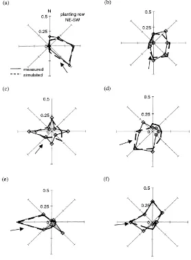
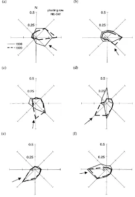
Fig. 3. Diurnal movement of sunflower canopy on 2 August 1998 (N indicates north; arrow indicates sun azimuth). (a) 10:30 hours, T=1.89, S=0.69, R=54.43◦; (b) 12:30 hours, T=0.81, S=0.59, R=64.17◦; (c) 14:30 hours, T=0.55, S=2.83, R=133.50◦; (d) 15:30 hours, T=1.15, S=0.73, R=170.17◦; (e) 17:00 hours, T=1.97, S=0.92, R=230.33◦; (f) 18:00 hours, T=1.40, S=1.35, R=255.54◦(note: T, S and
R are thickness, shape and rotation index, respectively).
experiment from 27 July to 26 August 1998. Fig. 3 shows a typical diurnal movement of sunflower from morning (about 10:30 hours; Fig. 3a) to late evening (about 18:00 hours; Fig. 3f) on 2 August. From morn-ing to noon (Fig. 3a and b), sunflower lagged the sun, with no parts of the sunflower canopy leading the sun. However, as the sun begun to align paral-lel to the planting row direction (about 14:30 hours; Fig. 3c), the canopy begun to disperse, orientating to a more random azimuth distribution. This dispersion
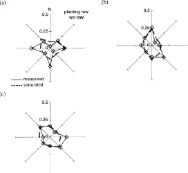
Fig. 4. Distribution of leaf azimuth density for sunflower when the sun was parallel to the planting row direction for the 1998 experiment (N indicates north). (a) 27 July, T=0.47, S=2.95, R=191.37◦; (b) 19 August, T=0.43, S=1.86, R=171.89; (c) 26 August, T=0.42, S=2.07, R=132.93◦(note: T, S and R are thickness, shape and rotation index, respectively).
elevation and irradiance was low, the canopy appeared to be shifting back to its normal or inert position.
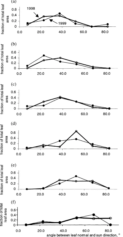
As the day progressed, the angle between sun-flower leaves (leaf normal direction) and sun direction increased (Fig. 5). This can be seen by the shift of distribution from left in the morning (Fig. 5a) to the right in the late evening (Fig. 5f). Observations were similar for both 1998 and 1999 experiments. In the
morning, most leaves were about 30◦ from the sun
direction (Fig. 5a). As the day progressed, this angle increased to about 50◦in the afternoon (Fig. 5d), and in the late evening, there was an increasing number of leaves that were 50◦or more from the sun direc-tion (Fig. 5f). These angles were larger from those reported elsewhere where the usual angle difference
observed was 20–30◦ (Polykarpov, 1954), 15–38◦
(Shell et al., 1974), or 25–35◦ (Ross, 1981). These differences were possibly due to differences in sun-flower varieties and growing conditions.
By varying the values of the leaf azimuth indexes (T, S, and R) of Eq. (3), the simulated densities matched the measured densities closely (Figs. 3 and
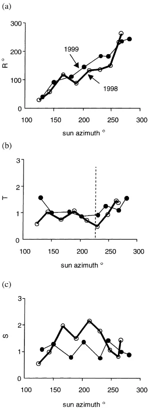
4). This is also shown in Fig. 6 where there was a close clustering of points along the 1:1 ratio line. The mean absolute estimation error AME for 1998 and 1999 experiments were 0.05 and 0.04, respectively. Plotting the estimation errors (simulated minus mea-sured) against the simulated values revealed no trend in estimation errors for both years (figure not shown). General relationships between the leaf azimuth indexes with sun position were sought. Of the three indexes, R had the most pronounced relationship with sun azimuth (Fig. 7a). The relationship between R and sun azimuth was linear for both years, and both having parallel linear slopes (slope of 1.2 for both 1998 and 1999 experiments). Varying R rotates the distribution around the origin. Thus, the linear rela-tionship between R and sun azimuth showed that R index had effectively characterised the solar-tracking movements of the canopy.
T index for both years were fairly constant (Fig. 7b).
Fig. 5. Diurnal changes to the distribution of angles between sunflower leaf normal and sun direction for the 1998 (2 August) and 1999 (8 July) experiment. (a) 10:30 hours; (b) 12:30 hours; (c) 14:30 hours; (d) 15:30 hours; (e) 17:00 hours; (f) 18:00 hours.
apparent that T would decrease sharply when the sun was parallel to the planting row direction. This was also observed, but less apparent, in the 1999 experi-ment, where T remained generally at minimum value as the sun gradually moved to a position parallel with the planting row. But as the sun moved away from this parallel position (after 13:30–14:30 hours), T would
Fig. 6. Comparison between simulated and measured leaf azimuth density for sunflower: (a) 1998, and (b) 1999 experiment.
increase again. This diurnal trend generally agreed with field observations. As stated earlier, progressively larger values of T produced distributions that are in-creasingly more elongated or ‘clumped’. Especially in the 1998 experiment, when the sun begun to align in parallel to the planting row, the distribution of leaf az-imuth density was observed to become progressively more circular or random (i.e. smaller T). But as the sun moved progressively further from the planting row direction, the density distribution was observed to be more clumped again (i.e. larger T).
Lastly, Fig. 7c shows the relationship between the
S index and sun azimuth. There was larger diurnal
Fig. 7. Relationship between sunflower leaf azimuth indexes with sun azimuth for the 1998 and 1999 experiments (dashed line in Fig. 7b indicates planting row direction).
fluctuations were also more uniform where the amount of increase in S was usually followed by a decrease of S in about the same amount. Consequently, S fluc-tuated rather uniformly about its mean value of 1.1. However, the fluctuations in the 1998 experiment were greater, and this indicated that the general shape of the azimuth density distribution (number of azimuth preferences) in the 1998 experiment was more vari-able than that in 1999.
In both experiments, azimuth density distribution generally tracked the sun in the same way (almost equal to R at a given sun position for both years), and the azimuth density distribution in the 1999 ex-periment was slightly more clumped than that in 1998 (slightly higher T for 1999 than 1998). The most obvi-ous difference between both experiments was S, where the sunflower canopy in the 1998 experiment would fluctuate between one to two azimuth preferences, but in the 1999 experiment, the sunflower canopy gener-ally showed one clear azimuth preference toward the sun direction (mean S of 1.1). Fig. 8 illustrates the mean azimuth densities for both years using the year’s respective mean values of T, S, and R. These three indexes were sensitive to the changes in azimuth den-sity distribution, and interpreting their diurnal changes complemented the interpretation of the distribution of angle difference between leaf normal and sun direc-tion as shown in Fig. 5. Though both years have rather similar diurnal distributions of angle difference be-tween leaf and sun, the changes in T, S, and R showed that there were some differences of azimuth density distributions between the two experiments.
This highlights the complex nature of heliotropism. Though both field experiments were set up to be the same, the growing conditions for both experiments were not. The growing condition during the data collection period for the 1998 experiment was drier (mean rainfall of 32 mm per month) than the 1999 experiment (mean rainfall of 54 mm per month). In addition, mean solar irradiance for the days when canopy architecture was measured in the first
exper-iment was 14 MJ/m2 per day. This was lower than
that in the 1999 experiment (mean solar irradiance
of 20 MJ/m2 per day). Ross (1981) observed that
Fig. 8. Mean leaf azimuth density for sunflower in the 1998 and 1999 experiments using the year’s respective mean values of the three indexes.
radiation interception; thus, reducing transpiration as well.
4.2. Leaf azimuth density of maize
As expected, maize canopies did not display any heliotropic behaviour. Comparing the azimuth den-sity distributions at different hours in a day (4–6 pe-riods) did not indicate any maize canopy movements or changes; that is, the azimuth distributions were
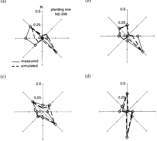
Fig. 9. Typical static distribution of leaf azimuth density for maize for the 1998 experiment. (a) 27 July, T=1.19, S=2.13, R=115.74◦; (b) 11 August, T=1.59, S=2.29, R=124.33◦; (c) 19 August, T=0.78, S=1.86, R=114.02◦; (d) 26 August, T=1.56, S=1.92, R=154.70◦ (note: T, S and R are thickness, shape and rotation index, respectively).
The simulated densities matched the measured den-sities closely with a clustering of points along the 1:1 ratio line (Fig. 10a and b). The mean absolute error of estimation AME was 0.05 and 0.04 for the 1998 and 1999 experiments, respectively. Plotting the esti-mation errors against the simulated values revealed no obvious trend in estimation errors for both years (fig-ure not shown).
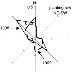
Unlike sunflower, the three leaf azimuth indexes for characterising the maize canopies were more constant because maize canopies did not follow the sun move-ment during the day. For the 1998 experimove-ment, the av-erage value of T was 1.4, S was 2.2, and R was 132◦. A S value of about 2 indicated two clear azimuth pref-erences with a distribution shaped like a ‘8’ (i.e. Fig. 1b); T of 1.4 indicated the maize distribution tended to be elongated (because most leaves were arranged at both opposite ends of the two azimuth preferences); and R of 132◦indicated an orientation that was almost perpendicular to the planting row direction. The mean indexes values for the 1999 experiment were almost equal to the 1998 experiment. For the 1999
experi-ment, the average value of T was 1.3, S was 2.1, and
R was 143◦. Fig. 11 shows the mean azimuth density distribution for maize for both 1998 and 1999 experi-ments using their respective mean values of the three indexes.
4.3. Crop classification
Logistic regression was used to determine how well the three leaf azimuth indexes discriminated
Table 1
Logistic regression analysis for crop classification (1998 experiment)a
Variable Coefficient Standard error Significance Odds ratio
T 3.247 0.984 0.001 25.720
S 2.664 0.797 0.008 14.349
R −0.003 0.007 0.642 0.997
Constant −8.601 2.573 0.008
Fig. 10. Comparison between simulated and measured leaf azimuth density for maize. (a) 1998 and (b) 1999 experiment.
Fig. 11. Mean leaf azimuth density for maize in the 1998 and 1999 experiments using the year’s respective mean values of the three indexes.
Table 2
Predicted crop classification using logistic regression (1998 exper-iment)
Actual classification Predicted classification Accuracy (%) Sunflower Maize
Sunflower 24 6 80.0
Maize 3 24 88.9
between sunflower and maize canopies. Table 1 shows the results of the logistic regression analysis for the 1998 experiment. Logistic regression revealed that these three indexes could be used to differentiate be-tween sunflower and maize canopies with a success rate greater than 80% (Table 2). Based on odds ra-tio (Table 1), the most important criteria or index to differentiate between sunflower and maize canopies was T, followed by S, then R. Odds ratio of an index is the increase in odds of being classified as a maize canopy for a unit increase of this index (everything else held constant). These results agreed with obser-vations that maize canopies usually had two clear azimuth preferences; were usually elongated (because leaves were mostly arranged at both opposite ends of the two azimuth preferences); and were usually orien-tated in a fixed position approximately perpendicular to the planting row. These three qualities of maize were generally uncharacteristic of sunflower. Similar results were obtained for the 1999 experiment, where
T, S, then R indexes were again identified as
impor-tant criteria to differentiate between sunflower and maize canopies. Success rate for crop classification for 1999 was also greater than 80%.
5. Conclusions
they had almost equal R index at a given sun az-imuth. However, the azimuth density distribution in the 1999 experiment (mean T of 1.2) was slightly more clumped than that in 1998 (mean T of 0.9), and that sunflower canopies in the 1998 experiment would fluctuate between one to two azimuth preferences (S between 0.6 and 2.2), but sunflower canopies in the 1999 experiment showed one azimuth preference (S between 0.8 and 1.4). For maize, mean T, S, and R for 1998 and 1999 were similar to each other (T=1.4 and 1.3, S=2.2 and 2.1, and R=132 and 143◦). These val-ues agreed with field observations because they also indicated that maize canopies were elongated, having two azimuth preferences that were perpendicular to planting row direction.
Further work on this equation is being planned especially to determine the possibility of linking the equation’s three azimuth indexes to any physical and biological plant basis, and the variability of these indexes in different environments. This equation is also being planned to be used in some detailed plant radiation models.
References
de Wit, C.T., 1965. Photosynthesis of Leaf Canopies. Agricultural Research Reports No. 663, Pudoc, Wageningen.
Ehleringer, J., Forseth, I., 1980. Solar tracking by plants. Science 210, 1094–1098.
Fukai, S., Loomis, R.S., 1976. Leaf display and light environment in row-planted cotton communities. Agric. Meteorol. 17, 353–379.
Jones, H.G., 1991. Plants and Microclimate: A Quantitative Approach to Environmental Plant Physiology, 2nd Edition. Cambridge University Press, Cambridge.
Lasdon, L.S., Waren, A., Jain, A., Ratner, M., 1978. Design and testing of a generalized reduced gradient code for nonlinear programming. ACM Trans. Math. Software 4, 34–50. Lemeur, R., 1973a. Effects of spatial leaf distribution on
penetration and interception of direct radiation. In: Slatyear, R.O. (Ed.), Proceedings of the Uppsala Symposium on Plants Response to Climatic Factors, 1970 (Ecology and Conservation 5). UNESCO, Paris, pp. 349–356.
Lemeur, R., 1973b. A method for simulating the direct solar radiation regime in sunflower: Jerusalem artichoke corn and soybean canopies using actual stand structure data. Agric. Meteorol. 12, 229–247.
Loomis, R.W., Williams, W.A., 1969. Productivity and the morphology of crop stands: patterns with leaves. In: Eastin, J.D., Haskins, F.A. Sullian, C.Y., van Bavel, C.H.M. (Eds.), Physiological Aspects of Crop Yield. Am. Soc. Agron., Madison, WI, pp. 27–47.
Polykarpov, G.G., 1954. Does blossoming sunflower head turn to the Sun? Sov. Nat. 5, 116–117 (in Russian).
Ross, J., 1981. The Radiation Regime and Architecture of Plant Stands. Dr. W. Junk Publishers, The Netherlands.
Ross, J., Nilson, T., 1966. Spatial orientation of leaves in plant canopy and its determination. In: Nichiporovich, A.A. (Ed.), Photosynthetic Systems with High Productivity. Engl. Trans. Israel Prog. Sci. Trans., Jerusalem, pp. 75–85.
Shell, G.S.G., Lang, A.R.G., 1975. Description of leaf orientation and heliotropic response of sunflower using directional statistics. Agric. Meteorol. 15, 33–48.
Shell, G.S.G., Lang, A.R.G., 1976. Movements of sunflower leaves over a 24 h period. Agric. Meteorol. 16, 161–170.