NETWORK DETECTION IN RASTER DATA USING MARKED POINT PROCESSES
A. Schmidt a, C. Kruse a, F. Rottensteiner a, U. Soergel b, C. Heipke a
a
Institute of Photogrammetry and GeoInformation, Leibniz Universität Hannover, Germany - (alena.schmidt, kruse, rottensteiner, heipke)@ipi.uni-hannover.de
b
Institute for Photogrammetry, University of Stuttgart, Germany - [email protected]
Commission III, WG III/4
KEY WORDS: Marked point processes, RJMCMC, graph, digital terrain models, networks
ABSTRACT:
We propose a new approach for the automatic detection of network structures in raster data. The model for the network structure is represented by a graph whose nodes and edges correspond to junction-points and to connecting line segments, respectively; nodes and edges are further described by certain parameters. We embed this model in the probabilistic framework of marked point processes and determine the most probable configuration of objects by stochastic sampling. That is, different graph configurations are constructed randomly by modifying the graph entity parameters, by adding and removing nodes and edges to/ from the current graph configuration. Each configuration is then evaluated based on the probabilities of the changes and an energy function describing the conformity with a predefined model. By using the Reversible Jump Markov Chain Monte Carlo sampler, a global optimum of the energy function is determined. We apply our method to the detection of river and tidal channel networks in digital terrain models. In comparison to our previous work, we introduce constraints concerning the flow direction of water into the energy function. Our goal is to analyse the influence of different parameter settings on the results of network detection in both, synthetic and real data. Our results show the general potential of our method for the detection of river networks in different types of terrain.
1. INTRODUCTION
Methods for automatic object detection can be subdivided into top-down and bottom-up approaches. For the latter, basic image processing methods such as segmentation are employed and the results are subsequently assigned to scene objects. In contrast, top-down approaches first express knowledge about the objects in suitable models and search for matches with the input data. Stochastic methods such as marked point processes (Møller J. and Waagepetersen R., 2004, Daley and Vere-Jones, 2003), which have been shown to achieve good results in various disciplines, belong to the top-down approaches. Marked point processes do not work locally, but rather find a globally optimal configuration of objects of a given type.
In the context of marked point processes, model knowledge about the objects to be detected can be expressed in different ways. In most cases, a simple geometric primitive which can be described by a small number of parameters is chosen to repre-sent an object in the scene. For instance, building contours are approximated by rectangles (Benedek et al., 2012, Chai et al., 2012, Tournaire et al., 2010, Ortner et al., 2007). The rectangles are distributed randomly in the input data and their conformity with the data is evaluated based on different criteria. In the cited papers, strong gradients of the grey values or heights at the rectangle borders and homogeneous values inside the rectangles are required for a rectangle to be accepted for the object con-figuration. Shadows are taken into account by evaluating the sun position (Benedek et al., 2012). Moreover, objects are re-quired not to overlap, and the model can be expanded to favour parallel objects (Ortner et al., 2007). Tournaire and Paparoditis (2009) as well as Li and Li (2010) also model objects by rectan-gles in the context of marked point processes. The former ex-tract dashed lines representing road markings from very high resolution aerial images, while the latter detect oil spills in synthetic aperture radar (SAR) data, integrating knowledge
about the distribution of the intensity in the backscattered radar signal. Alternative models are based on ellipses and circles, which were used by Perrin et al. (2005) to detect contour lines of tree crowns in optical data, whereas Descombes et al. (2009) applied such models to detect birds. The authors of both papers penalise overlapping objects and prefer a regular arrangement of the objects. Various geometric primitives are simultaneously considered in (Benedek and Martorella, 2014). The authors use lines and groups of points for the automatic detection of moving ships and airplanes in SAR images. First, the images are classi-fied into foreground and background; subsequently the models are fitted to the foreground pixels using marked point processes. Lafarge et al. (2010) developed a flexible approach for the detection of different types of objects in images. The authors set up a library composed of simple geometric patterns such as rectangles, lines and circles, which are defined by their lengths, orientations or radii. Here, the input data are evaluated based on the mean and standard deviation of the grey values inside and outside the proposed objects as well as the overlapping area between them. The authors report good results for different application such as the extraction of line networks, buildings and tree crowns.
The papers listed so far aim to detect isolated objects. Most of them model the objects as non-overlapping geometric primitives with similar image features or regular arrangement. For the detection of objects with a network structure, e.g. rivers and streets in remote sensing and blood vessels in medical data, the connectivity of objects can be integrated as an additional object property. This has been done in a number of studies which aim at the automatic detection of networks using marked point processes. Most of them are based on the Candy model devel-oped by Stoica et al. (2004), consisting of line segments having a certain width; two line segments are considered to be con-nected if the smallest Euclidian distance between their end-points is smaller than a predefined threshold. In the optimization The International Archives of the Photogrammetry, Remote Sensing and Spatial Information Sciences, Volume XLI-B3, 2016
process, the line segments are modified by changing their lengths and widths. Moreover, new line segments are added to or removed from the configuration. For the evaluation of each object configuration, segments which are not connected to other segments on both sides are penalised. The objects are also pe-nalised if they overlap, are too short, or enclose a small angle. The conformity of the object hypotheses with the input data is evaluated based on the homogeneity of the grey values of the pixels inside the segments and the grey value differences to the pixels outside the segment. These criteria can be adapted to the characteristics of the input data and, thus, good results for both, optical and SAR data are achieved. The authors succeed in detecting the major part of streets and river networks of their test data. Lacoste et al. (2005) refine the method and avoid constant penalisation terms by evaluating the segment configu-ration depending on the angle and the distance between two adjacent segments. Furthermore, the conformity with the input data is evaluated based on statistical tests. The authors detect street networks in optical images with a low false alarm rate even in case of occlusions by trees. However, the percentage of omission is quite high. For river networks, the authors observe large geometrical differences to the reference data, which are explained by the strong sinuosity of the rivers in the network. A similar approach is used by Sun et al. (2007) to detect vessels in medical data. The authors integrate the so-called vesselness in the evaluation of each segment, which is measured based on the eigenvalues of the Hessian matrix of the pixels values. An expansion of the Candy model to 3D data is realised by Stoica et al. (2007) and Kreher (2007), modelling the objects by cylin-ders instead of line segments.
In contrast to the methods mentioned above, Chai et al. (2013) model the network as a graph whose nodes correspond to junc-tion-points. In the sampling process, the nodes are iteratively connected by edges, which correspond to line segments and may have different widths. The edges are evaluated based on the homogeneity of the grey values inside the segments and the gradient magnitudes on the segment borders. The authors penal-ise graph configurations with non-connected components, atypical intersection angles and atypical numbers of outgoing edges (both compared to training data).
In this paper, we aim to take advantage of the benefits of marked point processes, i.e. the fact that they deliver a globally optimal solution and their flexibility thanks to the stochastic nature of the approach, in order to detect networks of rivers and tidal channels. Our input data are digital terrain models (DTM) derived from lidar point clouds. For that purpose, we extend the approach of Chai et al. (2013) to our application. As a novel feature and in comparison to our previous work (Schmidt et al., 2015), we integrate a model for the water flow direction and show its merits for the chosen application. In the following, we first describe the mathematical foundation of stochastic optimi-zation using marked point processes (Section 2). We then pre-sent the employed models for detecting rivers and tidal channel networks (Section 3). In Section 4, we show some experiments for data with varying terrain. Finally, conclusions and perspec-tives for future work are presented.
2. THEORTICAL BACKGROUND 2.1 Marked point processes
Point processes (for details see Møller and Waagepetersen, 2004 and Daley and Vere-Jones, 2003) belong to the group of stochastic processes. They are used for the description of phenomena which have a random characteristic, and, thus,
cannot be described in a completely deterministic way. A point process is a sequence of random variables , , where is the parameter set of the process. It is often represented by the time or location of the process (we are concerned with location here). takes values of the state space . In object extraction, point processes are used to find the most probable configuration of objects in a scene given the data. An object is described by its location li. In a marked point process, a mark mi, a
multidimen-sional random variable describing an object of a certain type at position li, is added to each point. If we characterise an object ui
= (li, mi) by its location and mark, a marked point process can
be thought of as a stochastic model of configurations of an unknown number n of such objects in a bounded region S (here: the DTM, thus the points li exist in = R
2 ).
There are different types of point processes. The Poisson point process ranks among the basic ones, it assumes a complete randomness of the objects, and the number ofobjects n follows a discrete Poisson distribution with parameter also called intensity parameter, which corresponds to the expected value for the number of objects. In the Poisson point process, adjacent objects do not interact. In practice, the assumption of complete randomness of the object distribution is often not justified, and more complex models are postulated instead. These models are described with respect to a reference point process, which is usually defined as the Poisson point process. In our model, we integrate interactions between adjacent objects by using Gibbs point processes, which are also applied in (Stoica et al., 2004), (Mallet et al., 2010) and others. In this setting the object con-figuration is described by a probability density function h which is related to a Gibbs energy U(.) to be minimised by
introduces prior knowledge about the object layout; our models for these two energy terms are described in Section 3.3. The
2.2 Reversible Jump Markov Chain Monte Carlo sampler Markov Chain Monte Carlo (MCMC) methods belong to the group of sampling approaches. The special feature of MCMC methods is that the samples are not drawn independently, but each sample Xt, , is drawn on the basis of a probability
distribution that depends on the previous sample Xt-1. Thus, the sequence of samples forms a Markov chain which is simulated in the space of possible configurations. If the number of objects constituting the optimal configuration were known or constant, it could be determined by MCMC sampling (Metropolis et al., 1953, Hastings, 1970). RJMCMC is an extension of MCMC that can deal with an unknown number of objects and a change of the parameter dimension between two sampling steps (Green, 1995). In each iteration t, the sampler proposes a change to the current configuration from a set of pre-defined types of changes. Each of the change types is associated The International Archives of the Photogrammetry, Remote Sensing and Spatial Information Sciences, Volume XLI-B3, 2016
with a density function Qi called kernel. Each kernel Qi is
reversible, i.e. each change can be reversed by applying another kernel. The types of changes and the kernels of our model are described in Section 3.2. A kernel Qi is chosen randomly
according to a proposition probability which may depend on the kernel type. The configuration Xt is changed according to
the kernel Qi, which results in a new configuration Xt+ 1.
Subsequently, the Green ratio R (Green, 1995) is calculated:
In (2), Ttis the temperature of simulated annealing in iteration t.
The kernel ratio
expresses the ratio of the probabilities for the change of the configuration from Xt+ 1 toXt
and vice versa, taking into account possible changes in the parameter dimension. Following Metropolis et al. (1953) and Hastings (1970) the new configuration Xt+ 1 is accepted with an
acceptance probability α and rejected with the probability 1-α, which is computed from R using
The four steps of (1) choosing a proposition kernel Qi, (2)
building the new configuration Xt+ 1, (3) computing the
acceptance rate α, and (4) accepting or rejecting the new configuration are repeated until a convergence criterion is achieved.
In order to find the optimum of the energy, the RJMCMC sampler is coupled with simulated annealing. For that reason, the parameter Tt referred to as temperature (Kirkpatrick et al.,
1983) is introduced in equation 2. The sequence of temperatures Tt tends to zero as . Theoretically, convergence to the
global optimum is guaranteed for all initial configurations X0 if
Tt is reduced (“cooled off”) using a logarithmic scheme. In
practice, a geometrical cooling scheme is generally introduced instead. It is faster and usually gives a good solution (Salamon et al., 2002, Tournaire et al., 2010).
3. METHODOLOGY
We use marked point processes with RJMCMC sampling and simulated annealing as described in Section 2 to detect a network of rivers or tidal channels. The network is modelled as an undirected graph whose nodes correspond to junction-points; the edges correspond to river or tidal channel segments. In the optimization process, the graph is iteratively changed and evaluated based on its conformity with a pre-defined model. We favour high DTM gradient magnitudes at the borders of the segments corresponding to the edges and we penalise confi-gurations consisting of non-connected components, overlapping segments, segments with atypical intersection angles and physically non-consistent networks.
In order to do so, three model specific definitions are required, which are described in the following subsections. First, we define the object representation of river and tidal channel networks (Section 3.1). Second, the types of change in the graph configuration which are applied during the sampling process are modelled (Section 3.2). Third, the energy function to be minimised during the global optimization is defined (Section 3.3). Note that the method presented in this paper is based on our previous work (Schmidt et al., 2015), where more details about some of these topics can be found.
3.1 Object model
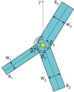
Our object model is based on an undirected graph. Similar to Chai et al. (2013) the nodes correspond to junction points. Each junction point possesses outgoing segments sj (j = 1,
..., ), see Figure 1 for nseg = 3. We characterize a junction
point by its image coordinates , and the orientation and width of each segment. The orientation is defined as counter-clockwise angle relative to the positive y-axis. In the sampling process, we iteratively build the graph by adding junction points to the configuration. If a new junction point is added in the neighbourhood of an existing one and fulfils some criteria (see Schmidt et al., 2015 for more details), both points are linked by a common segment. Such a segment is also added to the graph as an edge. Note that in particular in the early stage of the sampling process, a segment does not necessarily correspond to an edge in the graph; this is only the case for segments linking two junction points.
Figure 1. Example for a junction point with nseg = 3 outgoing
segments. Each segment sj is characterized by its width wj and
its direction βj.
3.2 Changes of the object configuration
In each iteration of the sampling process, we modify the graph describing the network of objects in the DTM. For that purpose, potential changes (also referred to as perturbations) that can be applied as well as the corresponding kernels Qi must be defined.
In this context, each perturbation is required to be reversible, i.e. for each perturbation there has to exist an inverse perturbation (Andrieu et al., 2003). We allow three types of change with related proposal probabilities pQM, pQT and pQB = pQD. On the
one hand, a node can be added to or removed from the current graph, which is accomplished by the birth-and-death kernel QBD.In the case of a birth event, all parameters are generated
based on learned probability density functions. Here, we assume a uniform distribution for each parameter (node position, number of segments, width and direction of each segment). The kernel ratio in equation (2) for this setting is
where pD and pB correspond to the probability for choosing a
birth or death event, respectively, λ is the intensity value of the Poisson point process which serves as reference process in our model (cf. Section 2.1) and n is the current number of nodes in the graph. For the death event, we model the kernel ratio by The International Archives of the Photogrammetry, Remote Sensing and Spatial Information Sciences, Volume XLI-B3, 2016
On the other hand, the parameters of the graph (node position, number of segments, width and direction of each segment) can be modified. In this study, we restrict the potential changes to changes of a junction point’s position and width; additional modifications are part of future research. For these events, associated with the translation kernel QT and themodification
kernel QM, respectively, the kernel ratio can be set to 1:
3.3 Energy model
3.3.1 Data Energy: The data energy Ud(Xt) (equation 1)
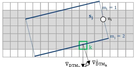
checks the consistency of the object configuration with the input data. Rivers and tidal channels are characterized by locally lower heights than their surroundings. Consequently, they are assumed to have high DTM gradient magnitudes on each bank and low gradient magnitudes in between. We determine the data energy from the DTM gradients at the segment borders by
In (7),
(see Fig. 2) is the component of the gradient of the DTM height at boundary pixel kj in direction of the normal
vector of the lateral edge mj {1, 2} of the segment sj (Figure
2). The sum of the gradients is taken over the nj pixels kj along
that edge; all gradients have equal weights. We only take into account the two lateral borders of the segment, potentially corresponding to the river or channel banks (bold lines in Fig. 2). To ensure that the value of the data term is above a predefined minimum value, we introduce a constant c.
3.3.2 Prior energy: Prior knowledge is integrated into the model in order to favour certain object configurations. We adopt the three terms of our previous work (see below and Schmidt el al., 2015) and in addition add a new term. The prior energy is thus modelled by
In (8) each term represents one of the characteristics of the network we intend to take into account in our model. In this way, a graph configuration with certain characteristics as pointed out in the subsequent paragraphs is favoured.
Non-overlapping segments: We penalise an object configuration in which the segments overlap. In this way, the accumulation of objects in regions with high data energy can be avoided. The corresponding energy term is calculated by the sum of the relative overlap area a of all combinations of segments si and sj
which are weighted by a penalising factor . Note that (1) we do not consider the overlap area of two segments which belong to the same junction point and (2) we only consider the larger relative overlap area of the two segments si and sj.
Graph connectivity: We want to obtain a configuration with only one graph and, thus, rate the connectivity of the nodes in the graph. For that purpose, we penalise all segments which do not link different nodes by
where ns is the number of segments in the graph which are
connected to only one node and ps is a constant penalising
factor.
Typical angles between edges: We favour intersection angles between edges which typically occur within river or tidal channel networks by
where na is the number of nodes which are linked by two or
more edges. For each of these nodes the angle between two edges is subtracted from the expected angle for the typical configuration which may be learned from the data or integrated as prior knowledge. The expected angle depends on the number of outgoing segments for each node, and pa is a
constant penalising factor.
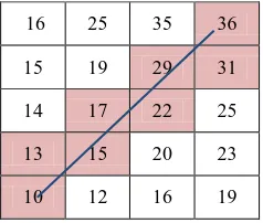
Physical consistency of the network: We take into account the flow direction of water by analysing the heights of the nodes and edges of the graph. The general idea is to take into account that water does not flow uphill. We integrate this physical knowledge using two criteria. First, each node needs to be connected by exactly one node with a lower height value but can have connections to an arbitrary number of nodes with a higher height value (Fig. 3) - this means that we do not consider basins, deltas or islands (which do not exist in our data) in our model. Second, each pixel on the medial axis of an edge has to show the same trend in the data, i.e. from the start to the end point all height values have to increase or decrease (Fig. 4); otherwise the edge is penalised. Note that we allow small deviations from this trend in order to be less susceptible to noise in the data. Thus, an edge is not penalised if the height of each pixel follows the trend of the edge within a tolerance of . Combining both criteria, the prior energy is modelled by
In (12) is the number of nodes violating the first criterion and is the number of edges violating the second criterion, whereas is a constant penalising factor.
Figure 2. The segment of a junction point (white circle) contributes to the data energy by the sum of the components of the gradients in the direction of the normal vector of each pixel k of the lateral edges. (The grey pixels indicate a channel / river in the DTM.)
.
Figure 3. Four nodes in a graph connected by edges. The arrows denote the flow direction of the water, determined on the basis of the heights at the junction points. For node 1 the first criterion is fulfilled: It has one neighbour with a lower height
and two neighbours with higher heights
.
25 35 36
15 19 29 31
14 17 22 25
13 15 20 23
10 12 16 19
Figure 4. DTM heights in a small local window, encoded by integer numbers. The upper right and the lower left corner of the window coincide with two junction points which are connected by an edge (blue line). The pixel values fulfil the second criterion: from the lower left corner to the upper right corner the height values grow continually (10-13-15-17-22-29-31-36).
4. EXPERIMENTS
We evaluate our method using three data sets (Section 4.1) for which we empirically set the parameters in our approach (Section 4.2). The aims of our experiments are twofold. First, we want to validate the energy function of our model by analysing the influence of each term (Section 4.3.). Second, we investigate the applicability of the method to data sets with completely different terrain types (Section 4.4).
4.1 Test data
For the evaluation of our method we use three data sets. Each of them consists of a DTM raster having a grid size of 1x1 m² (data set 1 and 2) and 0.5 x 0.5 m² (data set 3). While the first data set is a synthetic one, the other ones are generated from a laser scanning point cloud by using interpolation methods. The first data set represents a tidal channel network and consists of 700 x 550 m². Tidal channels are a special type of river furrowing the mudflat areas in coastal zones. A main characteristic of tidal channels is that they often form dendritic networks and exhibit a hierarchical structure in such a way that two smaller channels typically join to form a larger channel. In order to validate our method concerning the flow direction of water, the synthetic data have idealized height values: from the smaller channels to the bigger ones the heights gradually decrease without any noise in the data. The second data set, covering an area of 440 x 150 m² in the German Wadden Sea, consists of real data from a tidal channel network. In comparison to the synthetic data, the borders of the channels are less clear. Here, the transition to land is smoother, especially for the small channels. In general, the height gradients in scenes with tidal channels are very low. The difference between the lowest and the highest value in the real test site (including the
land) is only 1.4 m. This is in contrast to the third data set, which shows a river network in Vorarlberg, Austria, covering an area of 2500 x 2500 m². Here, the terrain is mountainous with height differences of nearly 250 m. For this data set also reference data for the medial axis of the river network are available. Experiments based on this DTM will help us to analyse the applicability of our method to scenes characterised by totally different terrain types.
4.2 Parameter settings
In our experiments, we set the parameters to values that were determined empirically based on our previous work (Schmidt et al., 2014, 2015). Unless noted otherwise, they are kept fixed for all tests. First, we give more weight to the prior energy than to the data term and, thus, set the parameter β in equation 1 to β = 0.09. The proposal probabilities of the kernels are set to pQM =
pQT= 0.45 and pQB = pQD = 0.05, whereas the probabilities for
choosing a birth or death event in equation 4 and 5 are pD = pB =
0.5. In order to speed up the computations, we set a threshold for the heights depending on the data and propose a new junction point in the birth event only at pixels whose height is below this threshold. The intensity parameter λ of the reference Poisson point process depends on the size of the test size is set to 30 (first and second data set) and 50 (third data set). For the prior knowledge about tidal channels we restrict the maximum width of a segment to the maximum width of channels in our scene which we manually measure in the data. The expected angles for adjacent edges are set to 180° or 135° for junction points with two segments which are the most common combination in our data. We calculate the difference for both values and take the smaller one for our prior term. For junction points with three segments (which is the maximum we allow) we use three values for the expected angles between the three segments, namely 180°, 135° and 45°, again using the smallest difference for the prior energy term. The parameter c in equation 7 is set to c = 200, and the initial temperature in equation 2 to Tt= 0 = 100. The standard values of the penalising
factors in the prior energy terms (equations 9-12) used for the three data sets are shown in Table 1. These values are used in the experiments described in Section 4.4, whereas in Section 4.3, where we want to assess the impact of the individual energy terms on the basis of the synthetic data set, we adapt these values as described in the text.
Table 1. Parameter settings of the penalising factors in the prior energy terms (equations 9-12).
4.3 Influence of each term in the energy function
Figure 5 shows how the object configuration in the synthetic data set evolves in the course of the sampling procedure, as junction points are added to or removed from the configuration or their parameters are changed. After 30 million iterations the tidal channel network is almost completely covered by segments (Fig. 5d). The contours of the channels correspond well to the borders of the segments, although the resultant graph is not completely connected.
Synthetic data
Wadden Sea
Austria
(overlapping areas) 2000 100 100 (non-connectivity) 100 100 100
(atypical angles) 10 5 1
(flow direction) 10 10 10
16
Figure 5. As the number of iterations t [in millions] increases, the tidal channel network is better and better described by the graph (green: junction points, yellow: their outgoing segments, red: edges in the graph).
Figure 6. Excluding the data term results in the construction of connected graphs which only consider data via the prior term for the flow direction. Increasing the corresponding penalising factor pf, the graph better and better approximates the channel
network.
Using the synthetic data set, we tested the influence of the individual terms of our energy function. First, we exclude the data term, so that only the prior knowledge about the charac-teristics of channel networks is taken into account. In this way, connected graphs are constructed in which the edges show the expected angles. Fig. 6a shows the results obtained when using the penalising factors in Table 1, except for the flow direction term, which is not considered (pf = 0). If we integrate
know-ledge about the flow direction, which does consider the DTM heights, the data have an impact on the result. The graph better and better approximates the network with increasing penalising factor . Figures 6b – 6d show the benefit of the results integrating the flow direction in the energy term.
We also analyse the influence of each prior term. By excluding the penalisation of overlapping areas, nodes and edges accumulate near the medial axes of the channels (Fig. 7). Segments with similar widths are sampled to nearly the same
positions. Thus, the graph does not represent the correct topology of the network. If we do not take into account the connectivity of the graph, the sampling results in several subgraphs (Fig. 8). Due to the data term, the segments still well coincide with the borders of the channels. However, we do not end up in a fully connected graph. Without consideration of typical angles in tidal channel networks, too many segments are added to the graph (Fig. 9). For instance, lots of junctions with degree 2 in the data are represented by nodes with degree 3 in the graph. If we exclude the term verifying the consistency of the flow directions (Fig. 10), the graph only slightly varies in comparison to the one in Figure 5d where all prior terms are taken into account. For the chosen weights, in our synthetic data the network is already well described by the further terms and the additional consideration of the flow direction does not significantly improve the results.
Figure 7. Results achieved by excluding the prior term penalising overlapping areas (po = 0).
Figure 8. Results achieved by excluding the prior term for graph connectivity (ps = 0).
Figure 9. Results achieved by excluding the prior term for typical angles (pa = 0).
= 0 = 1
10 = 1000
a) b)
c) d)
t = 1
t = 15 t = 30
a) b)
c) d)
Figure 10. Results achieved by excluding the prior term for the flow direction (pf = 0).
4.4 Applicability for different terrain types
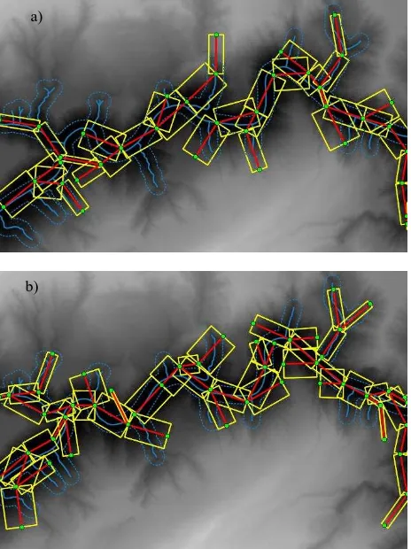
We also apply our approach to real data, using the values given in Table 1 for the penalising factors. Moreover, we adapt the maximum width a segment is allowed to have in the sampling process. For the Wadden Sea data, the graph describes the main tidal channel in the scene well: it is nearly completely covered by segments (Fig. 11a). Also some of the smaller channels are detected. By excluding the prior term for the flow direction, the number of detected small inlets increases (Fig. 11b). However, one segment (blue ellipse in Figure 11a and 11b) decreases in quality as it does not describe the correct route (and physical consistent flow) of the channel. For the third test site in Austria, reference data are available. We use the reference data for the evaluation and, first, only select all rivers which are below the threshold for the heights (see Section 4.2). We then derive a puffer with a width of 50 m and define all edge pixels lying in the puffer as correctly detected network parts. The completeness of the network is defined by all pixels of the reference network lying in the segments of our result. In this way, the completeness and correctness of our result are 71.7% and 90.2%, respectively, by using all prior terms (Fig. 12a). If we exclude the prior term for the flow direction, the completeness increases to 85.9% (Fig. 12b). However, the correctness decreases to 75.2% and, thus, shows the significance of this term.
5. CONCLUSION AND OUTLOOK
In this paper, we present a stochastic approach based on marked point processes for the automatic extraction of networks in raster data. We model the network as an undirected, acyclic graph which is iteratively built during the optimization process. The approach is evaluated on synthetic data and on two DTM derived from airborne lidar data. Our experiments showed that for all data sets, the most relevant tidal channels and rivers are detected, apart from some smaller inlets. In most cases, we end up in one single graph or only a small number of subgraphs. We also analysed the influence of the terms in our energy function and showed their relevance for the detection of river networks. The result decreases in quality if one of the terms is omitted. By integrating knowledge about the flow direction the results for the synthetic data and the DTM of the Wadden Sea are only slightly affected. However, for the mountainous test site the correctness of the detected network could be significantly improved by integrating this knowledge. Moreover, the application to different scenes with completely different terrain types demonstrated the transferability of our method.
In the future, we want to improve the strategy of adding new objects to an existing configuration. In our approach, junction
points are only proposed at pixels whose height is below a threshold. While this value helps to speed up the computation for the Wadden Sea data (where all channels have similar heights), the value is not meaningful for the Austria test site. We intend to replace it by a value based on terrain curvature. Furthermore, the reduction of parameters and the automatic learning of these parameters from training data are relevant topics.
Figure 11. Results for real data of a tidal channel network using (a) all prior terms and (b) by excluding the prior term for the flow direction (pf = 0).
Figure 12. Results for the test site in Austria using (a) all prior terms and (b) by excluding the prior term for the flow direction (pf = 0). Blue solid lines: reference data of the medial axes of
the river network, blue dotted line: puffer for evaluation. a)
b)
a)
b)
ACKNOWLEDGEMENTS
We would like to thank the State Department for Waterway, Coastal and Nature Conservation (NLWKN) of Lower Saxony for providing the Wadden Sea data and the State Office of Surveying and Geoinformation of Vorarlberg, Austria (http://www.vorarlberg.at/lvg), for providing the lidar and the reference data of Vorarlberg.
REFERENCES
Andrieu, C., 2003. An Introduction to MCMC for Machine Learning. Machine Learning, 50, pp. 5-43.
Benedek, C., Descombes, X., Zerubia, J., 2012. Building development monitoring in multitemporal remotely sensed image pairs with stochastic birthdeath dynamics. IEEE Transactions on Pattern Analysis and Machine Intelligence, 34 (1), pp. 33-50.
Benedek, C., Martorella, M., 2014. Moving target analysis in ISAR image sequences with a multiframe marked point process model. IEEE Transactions on Geoscience and Remote Sensing, 52 (4), pp. 2234-2246.
Chai, D., Förstner, W., Ying Yang, M., 2012. Combine Markov Random Fields and marked point processes to extract building from remotely sensed images. In: ISPRS Annals of Photogrammetry, Remote Sensing and Spatial Information Sciences, XXII-I-3 (September): pp. 365-370.
Chai, D., Förstner, W., Lafarge, F., 2013. Recovering line-networks in images by junction-point processes. IEEE Conference on Computer Vision and Pattern Recognition (CVPR), pp. 1894-1901.
Daley, D., Vere-Jones, D., 2003. An Introduction to the Theory of Point Processes: Volume I: Elementary Theory and Methods. New York, Berlin, Heidelberg, Springer, 2nd edition.
Descombes, X., Minlos, R., Zhizhina, E., 2009. Object extraction using a stochastic birth-and-death dynamics in continuum. Journal of Mathematical Imaging and Vision, 33 (3), pp. 347-359.
Green, P., 1995. Reversible Jump Markov Chains Monte Carlo computation and Bayesian model determination. Biometrika, 82(4), pp. 711–732.
Hastings, W., 1970. Monte Carlo sampling using Markov chains and their applications. Biometrika, 57(1), pp. 97–109.
Kirkpatrick, S., Gelatt, C. D., Vecchi, M. P., 1983. Optimization by Simulated Annealing. Science 220(4598), pp. 671-680.
Kreher, B.W., 2007. Detektion von Hirnnervenfasern auf der Basis von diffusionsgewichteten Magnetresonanzdaten. PhD thesis, Albert-Ludwigs-Universität Freiburg im Breisgau, Germany.
Lacoste, C., Descombes, X., Zerubia, J., 2005. Point processes for unsupervised line network extraction in remote sensing. IEEE Transactions on Pattern Analysis and Machine Intelli-gence, 27(2), pp. 1568–1579.
Lafarge, F., Gimel'Farb, G., Descombes, X., 2010. Geometric feature extraction by a multimarked point process. IEEE Transactions on Pattern Analysis and Machine Intelligence, 32 (9), pp. 1597-1609.
Li, Y., Li, J., 2010. Oil spill detection from SAR intensity imagery using a marked point process. Remote Sensing of Environment, 114 (7), pp. 1590-1601.
Mallet, C., Lafarge, F., Roux, M., Soergel, U., Bretar, F. Heipke, C., 2010. A marked point process for modeling lidar waveforms, IEEE Transactions on Image Processing, 19 (12), pp. 3204–3221.
Metropolis, M., Rosenbluth, A., Teller, A., and Teller, E., 1953. Equation of state calculations by fast computing machines, Journal of Chemical Physics, 21(6), pp. 1087–1092.
Møller, J., Waagepetersen, R., 2004. Statistical inference and simulation for spatial point processes. Chapman & Hall/CRC, Boca Raton, Fl., USA.
Ortner, M., Descombes, X., Zerubia, J., 2007. Building outline extraction from digital elevation models using marked point processes. International Journal of Computer Vision, 72 (2), pp. 107-132.
Perrin, G., Descombes, X., Zerubia, J., 2005. Adaptive simulated annealing for energy minimization problem in a marked point process application. Proc. Energy Minimization Methods in Computer Vision and Pattern Recognition, St Augustine, United States, Springer, Berlin-Heidelberg, Germany, 3757, pp. 3-17.
Salamon, P., Sibani, P., Frost, R., 2002. Facts, Conjectures and Improvements for Simulated Annealing. Society for Industrial and Applied Mathematics, Philadelphia, USA.
Schmidt, A., Rottensteiner, F., Soergel, U., Heipke, C. , 2014. Extraction of fluvial networks in lidar data using marked point processes. In: The International Archives of the Photogrammetry, Remote Sensing and Spatial Information Sciences XL-3, ISPRS Technical Commission III Symposium, Zurich, Switzerland, September 2014, pp. 297-304.
Schmidt, A., Rottensteiner, F., Soergel, U., Heipke, C., 2015. A graph based model for the detection of tidal channels using marked point processes. The International Archives of the Photogrammetry, Remote Sensing and Spatial Information Sciences, XL-3/W3, pp. 115-121.
Stoica, R., Descombes, X., Zerubia, J., 2004. A Gibbs point process for road extraction from remotely sensed images. International Journal of Computer Vision, 57 (2), pp.121-136.
Stoica, R., Martínez, V., Saar, E., 2007. A three-dimensional object point process for detection of cosmic laments. Journal of the Royal Statistical Society. Series C: Applied Statistics, 56 (4), pp. 459 - 477.
Sun, K., Sang, N., Zhang, T., 2007. Marked point process for vascular tree extraction on angiogram. IEEE Conference on Computer Vision and Pattern Recognition (CVPR), pp. 467– 478.
Tournaire, O., Paparoditis, N., Lafarge, F., 2009. Rectangular road marking detection with marked point processes. The International Archives of Photogrammetry, Remote Sensing and Spatial Information Sciences, XXXVI-3/W49A, pp. 73–78.
Tournaire O., Bredif, M., Boldo D., Durupt, M., 2010. An efficient stochastic approach for building footprint extraction from digital elevation models. ISPRS Journal of Photogrammetry and Remote Sensing, 65 (4), pp. 317 -327. The International Archives of the Photogrammetry, Remote Sensing and Spatial Information Sciences, Volume XLI-B3, 2016
![Figure 5. As the number of iterations t [in millions] increases, the tidal channel network is better and better described by the graph (green: junction points, yellow: their outgoing segments, red: edges in the graph)](https://thumb-ap.123doks.com/thumbv2/123dok/3288759.1403272/6.595.307.518.595.727/figure-iterations-millions-increases-described-junction-outgoing-segments.webp)