Explicit solution of a free boundary problem for
a nonlinear absorption model of mixed
saturated–unsaturated flow
Adriana C. Briozzo & Domingo A. Tarzia*
Departamento de Matema´tica, F.C.E., Universidad Austral, Paraguay 1950, (2000) Rosario, Argentina
(Received 11 November 1996; revised 23 March 1997; accepted 13 June 1997)
In wet soils, zones of saturation naturally develop in the vicinity of impermeable strata, surface ponds and subterranean cavities. Hydrology must be then concerned with transient flow through coexisting unsaturated and saturated zones. The models of advancing saturated zones necessarily involve a nonlinear free boundary problem.
A closed-form analytic solution is presented for a nonlinear diffusion model under conditions of ponding at the surface. The soil water diffusivity is restricted to the special functional form D(v)¼a=(b¹v)2, where v is the water content field to be determined and a, b are positive constants. The explicit solution depends on a parameter C (determined by the data of the problem), according to two cases: 1,C,C1 or C$C1, where C1 is a constant which is obtained as the unique solution of an equation. This result complements the study given in P. Broadbridge, Water Resources Research, 1990, 26, 2435–2443, in order to established when the explicit solution is available. The behavior of the bifurcation parameter C1 as a function of the driving potential is studied with the corresponding limits for small and large values. Moreover, the sorptivity is proven to be continuously differentiable function of the variable C.q1998 Elsevier Science Limited. All rights reserved
Key words: free boundary problem, mixed saturated–unsaturated flow, nonlinear absorption model.
1 INTRODUCTION
Following refs1,6, we consider a homogeneous soil which initially has some uniform volumetric water contentvn. At
times t .0, water is supplied at the surface x ¼0 under pressure head W0. Then, a mixed saturated–unsaturated
flow problem representing absorption of water by a soil with a constant pond depth at the surface is presented. At every time t the zone of saturation extends from x¼0 to x¼
s(t) (the free boundary), and the unsaturated zone extends for x.s(t). By assuming the Darcy’s law and neglecting the
gravity, the water flux is given by
v¼ ¹K(W)]W
]x, (1)
where W is the soil water matric potential and K is the hydraulic conductivity.
In the saturated zone we have1
W(x,t)¼W0¹
W0¹Ws
s(t) x; 0,x,s(t); (2)
and, the following free boundary problem eqns (3)–(7) arises for the unsaturated zone7:
v(s(t)þ,t)¼vs, t.0, (3) ]v
]t¼
]
]x D(v)
]v
]x
, x.s(t), t.0, (4)
¹Dð Þv ]v ]x s(t)
þ,t
ÿ
¼Ks
W0¹Ws
s(t) , t.0, (5)
v(x,0)¼v(þ`,t)¼vn, x.s(t), t.0, (6)
s(0)¼0 (7)
Printed in Great Britain. All rights reserved 0309-1708/98/$19.00 + 0.00 PII: S 0 3 0 9 - 1 7 0 8 ( 9 7 ) 0 0 0 2 6 - 2
713
where
.
x spatial coordinate
t time
v volumetric water content vn initial volumetric water content vs volumetric water content at saturation W soil water matric potential
W0 pond depth
Ws soil water potential at x¼s(t),Ws,W,W0 K hydraulic conductivity
Ks hydraulic conductivity at saturation D soil water diffusivity D¼KdW
dv
From now on we consider the free boundary problem eqns (3)–(7), where the position s(t) of the free boundary and the water fieldv(x,t) must be determined. We restrict our attention to the special functional form of the soil water diffusivity expressed by
D(v)¼ a
(b¹v)2 (8)
where a and b are positive constants. With this form of diffusivity, the nonlinear diffusion eqn (4) may be trans-formed in a linear one. Following ref.2, we normalize the water content variable as follows
Q¼ v¹vn
vs¹vn
(9) and we consider
C¼ b¹vn
vs¹vn
.1 parameter;
ls¼
a
(vs¹vn)C(C¹1)Ks
length scale;
ts¼
a C(C¹1)K2
s
time scale;
xp¼ x
ls
dimensionless length;
tp¼ t
ts
dimensionless time: 8
> > > > > > > > > > > > > > > > <
> > > > > > > > > > > > > > > > :
(10)
Then, problem eqns (3)–(7) is transformed into problem eqns (11)–(15)
]Q
]tp¼
]
]xp
C(C¹1)
(C¹Q)2
]Q
]xp
, xp.s
p(tp), tp.0, (11)
sp(0)¼0, (12)
Q(xp,0)¼Q(þ`,tp)¼0, xp.sp(tp), tp.0, (13)
Q(s p(tp)
þ,
tp)¼1, tp.0, (14)
¹C(C¹1)
(C¹Q)2
]Q
]xp sp(tp) þ,t
p
ÿ
¼W0p¹Wsp
sp(tp) , tp.0,
(15)
where
sp(tp)¼s(t)
ls
¼s(tstp)
ls
(16) is the position of the free boundary.
Now we define a dimensionless depth coordinate moving with the saturated–unsaturated interface
yp¼xp¹sp(tp).0, t
p¼tp.0; (17)
hence, we have the dimensionless free boundary problem eqns (18)–(22)
]Q
]t p
¼ ]
]y p
C(C¹1)
(C¹Q)2
]Q
]y p
þdsp
dtp
]Q
]y p
, yp.0, tp.0, (18) sp(0)¼0, (19)
Q(yp,0)¼Q(þ`,tp)¼0, yp.0, tp.0, (20)
Q(0,tp)¼1, tp.0, (21)
¹C(C¹1)
(C¹Q)2
]Q
]yp 0
þ,
tp
ÿ
¼Wop¹Wsp
sp(tp) , tp.0, (22)
where
W0p¼ W0
ls
dimensionless pond depth
Wsp¼ Ws
ls
dimensionless soil water potential at the moving saturated¹unsaturated interface:
The goal of the paper is to solve the dimensionless free boundary problem eqns (18)–(22). We will show an expli-cit to this problem which depends on a parameter C, according to two cases: 1,C,C1 or C$C1, where C1
is a constant (the bifurcation parameter) obtained as the unique solution of the following equation:
Q d 2
C¹1
p
¼ 2
C, C.1, (23)
where Q is a real function defined by Q(x)¼pp
xexp(x2)erfc(x), x.0, (24)
andd.0 is a parameter defined in eqn (43).
2 CLOSED-FORM ANALYTIC SOLUTION OF THE FREE BOUNDARY EQNS (18)–(22).
In order that the two boundary conditions eqns (3) and (5) are compatible, s(t) must be of the form
s(t)¼mpt, (25)
m being an unknown constant. By eqns (2) and (5), the
following expression
m¼2Ks W0¹Ws
ÿ
S , (26)
and v(s(t),t)¼S=2pt is the infiltration rate, where v is
related to W through the Darcy eqn (1). The sorptivity S is a basic hydraulic property relating cumulative intake I(t) (expressed as a length) to the square root of time for a one-dimensional sorption into a soil without gravity, i.e. I(t)¼Spt (Ref. 8). It has been shown in4,5that the domi-nant parameter governing the dynamics of infiltration at small times is the sorptivity S. Since S ia measure of the capil-lary uptake or removal of water, is essentially a property of the medium with some resemblance to permeability. When v is in cm s¹1and t in s, the unit of S is cm s¹12(Ref. 4).
Then, in terms of dimensionless variables we have sp(tp)¼mpptp (27) To linearize the diffusion eqn (4) we define the variables3
m¼C(C¹1)
and we obtain the problem eqns (30)–(33)
]m
Now we assume a similarity solution
m¼g(f), f¼ x
t
p : (35)
Then the problem eqns (30)–(33) reduces to the problem eqns (36)–(39)
The solution to the conditions eqns (36)–(38) is given by g(f)¼C¹1þCS where the coefficient gis unknown.
The extra boundary condition eqn (39) is consistent with this solution provided that
1
Since S andgverify the following relation (another method is given in Remark 3 and Appendix A)
S¼
In studying eqn (44), we shall consider two cases respec-tively corresponding to choose the sign (þ) or (¹).
Case 1: (sign þ in the expression of S as a function ofg) The eqn (44) may be written as
1
where H1 is defined by
H1(g,C)¼
Now we define the real function F1(g,C)¼
1
CH1(g,C)
, g$g0(C), C.1: (48)
which satisfies the following properties
(i) F1(g0(C),C)¼
Then, we have that the eqn (45) is equivalent to
F1(g,C)¼Q
g
2
, g$g0(C), C.1: (50)
Since Q satisfies the properties
(i) Q(0)¼0,
we conclude that eqn (50) admits a unique solution in the variablegif and only if
F1(g0(C),C)¼
where the real function M is defined by M(C)¼CQ g0(C) The function M satisfies the following properties
(i) M9(C).0, C.1,
Therefore, there exist a unique constant C1.1 such that
M(C1)¼C1Q
Moreover, by using eqn (53)iv we deduce
C1.2 (55)
Case 2: (sign ¹ in the expression of S as a function ofg) The eqn (44) may be written as
1
where H2 is defined by
H2(g,C)¼
which satisfies the following properties
(i) H2(g0(C),C)¼
Now we define the real function F2(g,C)¼
1
CH2(g,C)
, g$g0(C), C.1: (59)
which satisfies the following properties
(i) F2(g0(C),C)¼
Hence, the eqn (56) is equivalent to F2(g,C)¼Q
g
2
, g$g0(C), C.1: (61)
Taking into account the properties of functions Q and F2,
we deduce that eqn (59) admits a unique solution in the variable gif and only if
F2(g0(C),C)¼
Then, we have obtained the following result:
Theorem 1. Assume that C¼ ðb¹vnÞ=ðvs¹vnÞ.1.
and, the solution of the problem eqns (36)–(39) is given by
II) If C$C1: There exist a uniqueg2(C)$g0(C)such that
and, the solution of the problem eqns (36)–(39) is given by
g2(f)¼C¹1þ
Therefore, the solution of the problem eqns (36)–(39) is given by
The sorptivity S as a function of the variable C is given by
S(C)¼
defined by eqns (62) and (65) respectively.
The function S¼S(C) is continuously differentiable.
Moreover, we have
S(1þ)¼ þ`, S(þ`)¼0: (72)
elementary but tedious computations we obtain
]S1
On the other hand, by elementary computations we get eqn (72).
Remark 3. An alternative method to prove Theorem 1 was suggested by an anonymous referee and it is shown in the Appendix.
Finally, we invert the relations eqns (35), (29), (10) and (9) to obtain the parametric solution to the problem eqns (3)–(7), which depends on C.
Corollary 2. There exists a bifurcation parameter C1¼C1(d)¼C1(a,Ks,W0¹Ws,vs¹vn).1, for the
solu-tion of problem (3)–(7) which is given by:
3erfc x tions coincide one each other, that is
v1(x,t)¼v2(x,t)¼(vs¹vn)C1 1¹
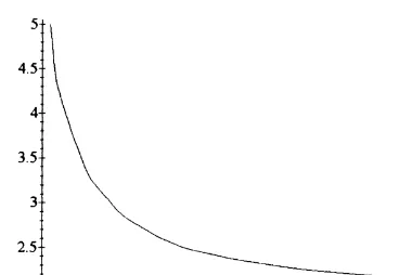
3 BEHAVIOR OF THE BIFURCATION
PARAMETER C1UPON THE DATA
solution of the eqn (23), as a function of the variable d
defined by eqn (43). See Fig. 1 and Table 1.
Lemma 3. We have that C1¼C1(d)satisfies the following properties:
(i) C1.2; (ii)
]C1
]d ,0, ;d.0;
(iii) lim
d→0þC1(d)¼ þ
`; (iv) lim
d→þ`C1(d)¼2 : 8
> <
> :
(91)
Moreover, we have that the inverse function d¼d(C1) is given explicitly by
d¼ 2
C1¹1
p Q
¹1 2 C1
, C1.2,
where Q¹1 is the inverse function of Q.
Proof.
(i) is the condition eqn (55). (ii) By using eqn (51) we have dC1
dd(d)¼
1 2
3
¹C1(d)
C1(d)¹1 p
Q9 d
C1(d)¹1 p
2
!
Q d
C1(d)¹1 p
2
!
þ C1(d)d
4 C1(d)¹1
p Q9
d C1(d)¹1 p
2
!
,0, d.0:
(iii) If the limit of C1ð Þd is finite whend→0
þ
we have a contradiction with eqn (23) because its left hand side goes to 0 and its right hand side goes to a positive number. Therefore eqn (91)iii holds.
(iv) If limd→þ`C1ð Þ ¼ þd `then we have a
contradic-tion with eqn (23) because its left hand side goes to 1 when dgoes to þ`(because of eqn (51)ii) while its right hand side goes to 0. Then, the limit of C1ð Þd is
finite ($2) whendgoes to þ`. Then, by eqn (51)ii, we get eqn (91)iv.
Analogously, we can study the bifurcation parameter C1
as a function of the driving potentialedefined by
e¼W0¹Ws (92)
Theorem 4. The function C1¼C1(e)satisfies the follow-ing properties:
(i) C1.2; (ii)
]C1
]e ,0, ;e.0;
(iii) lim
e→0þC1(e)¼ þ
`; (iv) lim
e→þ`C1(e)¼2 : 8
> <
> :
(93)
Proof. By taking into account the Lemma 4, and the
param-eters dandeare related by the following expression
d¼
me
p ,
withm¼8Ks vs¹vn
ÿ
a (94)
the results (i)–(iv) hold.
From Theorem 5 we obtain the following conclusions: (i) It is clear that only the ‘þ’ branch, in relation eqn (42), occurs when the driving potential e¼W0¹Ws
goes to zero because of eqn (93)iii). Therefore, the ‘¹’ branch has not physical meaning.
(ii) For the other cases (the driving potential
e¼W0¹Ws is positive) the two branches (‘þ’ and
‘¹’) in relation (42) have a physical meaning.
ACKNOWLEDGEMENTS
This paper has been sponsored by the Project #4798 Free
Boundary Problems for the Heat-Diffusion Equation from
CONICET, Rosario-Argentina. The authors appreciate the valuable suggestions by two anonymous referees which improved the paper.
Fig. 1. The bifurcation parameter C1 versus variable which are related by the eqn (23).
APPENDIX A
We shall show a new proof of Theorem 1 by studying a single trascendental equation for the sorptivity S. If we sub-stitute eqn (34) in eqn (41), we obtain for the unknown S the following equation
F(S,C)¼Qp(S,C), S.0 (C.1 : parameter) (A1)
where
F(S,C)¼g(S,C)
a p
CS ¼
1
Cþ
ad2(C¹1)
4S2C , S.0, C.1
(A2) and
Qp(S,C)¼Q g(S,C)
2
, S.0, C.1 (A3)
with
g(S,C)¼ S
a
p þ
a p
d2(C¹1)
4S , S.0, C.1 (A4) By elementary computations we deduce that the functions
Qpand F satisfy the following properties.
Lemma 5. We have:
(i)
Qp(0,C)¼Qp(þ`,C)¼1, C.1
; (ii)
]Qp ]S(S,C)¼
,0 if S,Sp, C.1
0 if S¼Sp, C.1 .0 if S.Sp, C.1
8
> > <
> > :
where
Sp¼Sp(C)¼
a p
2 g0(C)¼
dpa(C¹1)
2 (A5)
is the minimum point of function Qp with respect to S, for
all C.1.
(iii) Qp(Sp,C)¼Q g0(C)
2
, C.1.
Lemma 6. We have:
(i)F(0,C)¼ þ`,C.1;(ii)F(þ`,C)¼ 1
C,C.1;
(A6)
(iii)]F
]S(S,C),0, S.0, C.1; (iv)F(S
p,C)¼ 2
C,
C.1:
Theorem 7. The eqn (A1) for the sorptivity S with a
parameter C.1, admits a unique solution Sp
1.Sp if
1,C,C1 or, Sp
2,Sp if C.C1, where C1 is the unique solution of the eqn (23).
Proof. Functions F and Qp satisfy the following
rela-tions:
(a)F(Sp,C).Qp(Sp,C)
⇔ 2
C.Q
g0(C)
2
⇔
M(C),2⇔1,C,C1: (b)F(Sp,C),Qp(Sp,C)
⇔ 2
C,Q
g0(C)
2
⇔
M(C).2⇔C.C1:
Therefore, for a fixed C, we have that if 1,C,C1 the
abscisa Sp
1 of the intersection point of the graphs of the
functions F and Qp is to the right of the minimum point
Sp(Sp
1.Sp), in other case this point Sp2 is to the left of the
minimum point (Sp
2,Sp).
Now, we can relate the solutions Sp1and Sp2of the eqn (A1)
according to the two cases 1,C,C1and C.C1
respec-tively, which are given by the above Theorem 8, with the expressions eqns (64) and (67) obtained in Theorem 1.
Theorem 8. We have
(i)Sp
1¼S1(C)¼ a p
2 g1(C)þ
g2 1(C)¹g
2 0(C) q
,
1,C,C1
(ii)Sp
2¼S2(C)¼ a p
2 g2(C)¹
g2
2(C)¹g20(C) q
,
C.C1
(iii)Sp
1¼Sp2¼S(C1)¼ a p
2 g0(C1)¼
d
2
a(C1¹1) p
¼ 2(W0¹Ws)(vs¹vn)(C1¹1) p
, C¼C1:
Proof. Sp
1 and Sp2 must satisfy the expression eqn (42). On
the other hand, for 1,C,C1 we have
Sp
1.Sp¼
a
p
2 g0(C). Then Sp1 is given by the sign ‘þ’ in
eqn (42) (analogously for C.C1 we have Sp
2 is given by
the sign ‘¹’ in eqn (42)) because the functions g3(x)¼xþ
x2¹g2
0(C) q
, g4(x)¼x¹
x2¹g2
0(C) q
,
x.g0(C)
satisfy the following properties: g3(g0(C))¼g4(g0(C))¼g0(C),
g3(þ`)¼ þ`, g4(þ`)¼0,
g39(x).0, g49(x),0:
REFERENCES
of mixed saturated-unsaturated flow. Water Resources Research, 1990, 26, 2435–2443.
2. Broadbridge, P. & White, I. Constant rate rainfall infiltration: A versatile nonlinear model. 1. Analytic solutions. Water Resources Research, 1988, 24, 145–154.
3. Knight, J. H. & Philip, J. R. Exact solutions in nonlinear difussion. J. Eng. Math., 1974, 8, 219–227.
4. Philip, J. R. The theory of infiltration. 4. Sorptivity and alge-braic infiltration equations. Soil. Sci., 1957, 84, 257–264. 5. Philip, J. R. The theory of infiltration. 5. The influence of the
initial moisture content. Soil. Sci., 1958, 85, 329–339.
6. Philip, J. R. The theory of infiltration. 6. Effect of water depth over soil. Soil. Sci., 1958, 85, 278–286.
7. Tarzia, D. A., A bibliography on moving-free boundary pro-blems for the heat-difussion equation. The Stefan problem. Progetto Nazionale M. P. I., Equazione di evoluzione e appli-cazioni fisico-matematiche, Firenze, 1988 (with 2528 refer-ences). An updated one will give at the end of 1997 with more than 5000 on the subject.