Non-generic aspects of optimizing measures
in dynamical systems
February 2019
A Thesis for the Degree of Ph. D. in Science
Non-generic aspects of optimizing measures
in dynamical systems
February 2019
Graduate School of Science and Technology
Mao Shinoda
Contents
1 Introduction 1
2 Symbolic Dynamical Systems 7
2.1 Definitions . . . 7
2.1.1 Subshifts, words and languages . . . 7
2.1.2 Vertex and labeled edge shifts . . . 8
2.2 Examples . . . 10
2.2.1 Subshifts of finite type . . . 10
2.2.2 Sofic shifts and factor maps . . . 10
2.2.3 β and (−β) shifts . . . 11
2.2.4 Dyck shifts . . . 13
2.3 Invariant measures on symbolic systems . . . 16
2.4 Coding . . . 17
3 Structure of invariant measures and convex functional technique 19 3.1 Borel probability measures . . . 19
3.2 Simplex structure of invariant measures . . . 20
3.3 The Bishop-Phelps theorem . . . 21
3.4 Uncountably many extremal points . . . 24
4 Main theorems 27 4.1 Uncountably many maximizing measures . . . 27
4.2 Uncountably many Lyapunov maximizing measures . . . 30
4.2.1 Proof of Theorem C . . . 31
4.2.2 Preliminaries . . . 32
4.2.3 On the proof of the Realization Theorem . . . 34
5 Zero temperature limit problem 45 5.1 Finite systems . . . 45
5.2 Infinite systems . . . 46
A The Ma˜n´e-Conze-Guivarc’h lemma 54
B Multidimensional symbolic systems 60
B.1 Setting . . . 60 B.2 Wang tiling . . . 61
Chapter 1
Introduction
A dynamical system is a mathematical model of a phenomenon following a deterministic law of time evolution, as typified by differential equations and difference equations. Theory of dynamical systems, which is originated in the study of the three-body problem by Poincar´e, was established after the study in the 1960s by Smale and the discovery of “chaos” in applied fields [Lo63, LY75]. In this thesis we consider a discrete time dynamical system defined by a continuous self-map of a compact metric space. Unless otherwise stated, X denotes a compact metric space and T :X →X denotes a continuous map.
One way to investigate behaviour of a system is to consider the time average of a function φ which measures its “performance” at each point, that is
lim n→∞ 1 n n−1 ! k=0 φ◦Tk(x),
where Tk denotes the k times iteration of the map T. An elementary example of a
“performance function” is the characteristic functionχA of a subsetA. The time average of χA along with the orbit of a point xis the frequency with which the orbit hits A:
lim n→∞ 1 n n−1 ! k=0 χA◦Tk(x) = lim n→∞ 1 n# " k = 0,1, . . . , n−1 :Tk(x)∈A#.
This limit is called the hitting frequency, if it exists. It is natural to ask which orbits maximize the time average of a performance function. The selection of orbits attaining the maximum time average is the main purpose of ergodic optimization. A root of this theory is found in the works of Mather [Mat91] and Ma˜n´e [Man96, Man97] on the dynamics of the Euler-Lagrange flow: orbits with prescribed properties can be obtained by the Lagrangian, and the orbits are obtained as typical points for these measures (called action minimizing measures, see [So15]). Another root is found in the selection of unstable optimal periodic orbits in chaos control [OGY90, HO96a, YH99]. Resent progress of ergodic optimization is nicely surveyed by Jenkinson [J06, J18].
The question of time average can be interpreted as that of space average via the Birkhoff ergodic theorem. For a real-valued continuous function φ :X →R we have
sup x∈X lim sup n→∞ 1 n n−1 ! k=0 φ◦Tk(x) = max ν∈MT $ φ dν, (1.1)
whereMT denotes the space of allT-invariant Borel probability measures. AT-invariant
Borel probability measure attaining the maximum is called a maximizing measure for φ. Hence we can restate the question: which invariant measures are maximizing measures for a performance function? If a system admits only one invariant measure, not only the above question becomes trivial but also the time average of a continuous function at any point uniformly converges to its space average by the unique invariant measure [Wa82, Theorem 6.19]. Hence the case where MT is not a singleton is of our interest.
The setMT of invariant measures is a non-empty convex and compact set with respect
to the weak*-topology [Wa82, Theorem 6.10]. We pay attention to a system for which the space of invariant measures has a complicated structure. For example, the space of invariant measures of a topologically mixing subshift of finite type is thePoulsen simplex, i.e. an infinite dimensional simplex where the set of extremal points is dense. Extremal points of MT are ergodic measures [Wa82, Theorem 6.10]. A σ-invariant measure is
ergodic if µ(A) = 0 or µ(A) = 1 for every Borel set A such that σ−1A = A. As we will see in Section 3.2, any invariant measure allows a unique integral representation by a probability measure supported on the set of ergodic measures.
It is usually difficult to detect maximizing measures for individual performance func-tions. As far as the knowledge of the author, such results are only known for special functions on the angle-doubling map [Bou00]. Most results in ergodic optimization are on “typicality” of properties for maximizing measures: How large subset is contained in the set of performance functions for which a property holds? An important formulation of this notion is genericity. A subset R of a topological space is residual if it is an intersection of countably many open and dense subsets. Let F be a Baire space, i.e. every residual subset is dense inF. By Baire’s category theorem, if F is a complete metric space, then it is a Baire space. In Theorems A and B, for example, we consider the space of continuous functions onX with the supremum norm asF. A propertyP for elements inF isgeneric
if the set of φ inF satisfying P contains a residual subset.
It is proved by Jenkinson that uniqueness of maximizing measure for continuous func-tions is generic [J06]. Moreover, the unique measure is fully supported and has zero entropy, provided T has specification property [BJ02, Br08, Mo08]. For more regular functions the dynamics on the support of a unique maximizing measure is supposed to be periodic. Indeed there are several positive results for Lipschitz continuous functions by Contreras [Co16] and by Bochi and Zhang [BZ15]; for super-continuous functions by Quas and Siefken [QS12]; for H¨older continuous functions by Contreras, Lopes and Thieullen [CLT01]; for continuous functions satisfying the Walters condition by Bousch [Bou01].
In contrast to these results, main results of this thesis shed some light on continuous functions with multiple maximizing measures.
It is interesting to see the relation between the existence of multiple maximizing mea-sures and thermodynamic formalism. For a continuous functionφ andβ ∈Ran invariant measureµ is an equilibrium measure for βφ if it attains the following supremum:
sup µ∈MT % hµ+β $ φ dµ &
wherehµ denotes the Kolmogorov entropy. We callβ the inverse temperature parameter.
For a given continuous function φ consider a sequence {µβ} of equilibrium measures for
βφ. As we will see in Chapter 5, maximizing measures naturally appear as zero tem-perature limits of equilibrium measures: any accumulation point of {µβ} as β goes to
infinity becomes a maximizing measure for φ. Hence the uniqueness of maximizing mea-sure implies convergence of {µβ}. On the other hand, the limit does not always exist:
Chazottes and Hochman give examples of Lipschitz continuous functions for which the sequence {µβ} does not convergence [CH10]. Paying attention to oscillation of
equilib-rium measures at low temperature, we should study continuous functions with multiple maximizing measures. Existence of multiple maximizing measures cannot be a generic property by Jenkinson’s result on generic uniqueness. However, our main results say that such functions exist densely in the space of continuous functions.
Denote byC(X) the space of continuous functions endowed with the supremum norm. Theorem A ([Sh17, Theorem A]). Let (X, T) be a topologically mixing subshift of finite type. Then there exists a dense subset D of C(X) such that for every φ in D there exist uncountably many ergodic maximizing measures which are fully supported and have positive entropy.
In Theorem A, the notion of uncountably many maximizing measures crucially changes when we drop ergodicity. Every convex combination of ergodic maximizing measures is also a maximizing measures. Hence we can obtain uncountably many maximizing measures which are not ergodic, if there exist at least two ergodic ones. In Theorem A we claim the existence of uncountably manyergodicmaximizing measures, which is much different from that of uncountably many merely maximizing ones. Theorem A is obtained by slightly modifying a proof of the following theorem.
Theorem B ([Sh17, Theorem B]). Let T be a continuous self-map of a compact metric space X. Suppose the set Me of all ergodic measures is arcwise-connected. Then there
exists a dense subset D of C(X) such that for every φ ∈D there exist uncountably many ergodic maximizing measures.
Property of the setMeof all ergodic measures depends on “hyperbolicity” ofT.
The space of invariant measures of these systems is actually the Poulsen simplex [Sig74]. The denseness of the set of ergodic measures implies its arcwise-connectedness because the Poulsen simplex and the set of its extremal points are homeomorphic to the Hilbert cube [0,1]∞ and its interior (0,1)∞ respectively [GK16]. In the one-dimensional case, Blokh shows that continuous topologically mixing interval maps have specification prop-erty [Bl83] and a discontinuous version is studied in [Bu97]. The arcwise-connectedness of the set of ergodic measures is strictly weaker than the denseness of it. For example the set of ergodic measures of a Dyck shift is not dense but arcwise-connected, as we will see in Subsection 2.2.4. The connectedness of the set of ergodic measures for some partially hyperbolic systems is studied in [GP15]. On the other hand, there do exist systems for which Me is not arcwise-connected: Cortez and Rivera-Letelier show that for the
restric-tions of some logistic maps to the omega limit set of the critical points, the sets of ergodic measures become totally disconnected [CR10].
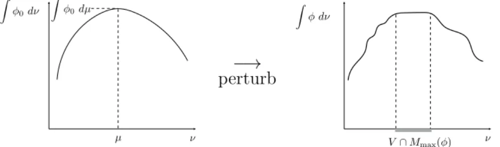
An idea of our proof of Theorem B is to perturb a given continuous function φ0 to create another continuous functionφso that the functionµ%→' φdµdefined on an arc of ergodic measures has a “flat” part (see Figure 1.1). The Bishop-Phelps theorem ensures such a perturbation. In order to use the Bishop-Phelps theorem, we use the fact that maximizing measures are characterized as “tangent measures” to the convex functional
Q:C(X)∋φ%→ max
ν∈MT
$
φ dν ∈R.
The use of the Bishop-Phelps theorem has been implied by [PU10] (see also [I79]).
0dµ µ 0d −→ perturb d V Mmax( )
Figure 1.1: A schematic picture of the perturbation of a performance function: a given function φ0 (left); the perturbed function φ (right).
Inspired by Theorem A we study existence of multiple Lyapunov maximizing mea-sures for piecewise expanding Markov maps. The dynamics of a piecewise expanding Markov map can be interpreted as that of a full shift by topological conjugacy. With this interpretation, we can apply Theorem A to the context of Lyapunov maximizing measure. We start with definition of piecewise expanding Markov maps. Letp≥2 be an integer
and {αi}pi=0−1,{βi}
p−1
i=0 sequences in [0,1] such that
0 =α0 <β0 <α1 <β1 <α2 <· · ·<βp−1 = 1.
PutX =(pi=0−1[αi,βi]. AC1 functionf :X →[0,1] is a piecewise expanding Markov map onX if it satisfies the following:
(E1) f maps each interval [αi,βi], i∈{0, . . . , p−1} diffeomorphically onto [0,1];
(E2) there exist constants) c > 0, λ > 1 such that for every n ≥ 1 and every x ∈
n−1
k=0f−k(X), |Dfn(x)|≥cλn.
Denote by E the space of piecewise expanding Markov maps on X endowed with theC1 topology given by the norm
∥f∥C1 = sup
x∈X|
f(x)|+ sup
x∈X|
Df(x)|.
As we will see in Section 4.2, the space E is an open subset of C1 functions on X, and hence becomes a (non-complete) Baire space.
Observe that there are points in X which cannot be infinitely iterated by f, because of gaps. Hence we restrict f toΛ(f) defined by
Λ(f) = *
n≥0
f−n(X).
Thus we obtain a dynamical system which is also denoted by f with a slight abuse of notation. Then Λ(f) is a Cantor set with a Markov partition given by the collection {[αi,βi]}ip=0−1 of intervals which topologically conjugates f to the full shift over psymbols. See Section 2.4 for more details.
Put χmax(f) = max µ∈Mf $ log|Df|dµ and χmin(f) = min µ∈Mf $ log|Df|dµ.
A measureµ∈Mf is Lyapunov maximizing if it is a maximizing measure for log|Df|:
$
log|Df|dµ=χmax(f).
Lyapunov minimizing measure is defined similarly, with χmax replaced by χmin. Since Lyapunov maximizing measure is defined for each maps, we discuss genericity or non-genericity with retard to maps instead of functions in the context of Lyapunov maximizing measure.
The notion of Lyapunov optimizing measures was introduced by Contreraset al[CLT01]. They showed that for an open dense subset of the space (β>αC1+β of expanding maps
of the circle in theC1+α topology, the Lyapunov maximizing measure is unique and
sup-ported on a periodic orbit. For a generic C1 expanding map of the circle, Jenkinson and Morris [JM08] proved that the Lyapunov maximizing measure is unique and has zero en-tropy. See Morita and Tokunaga [MT13], Tokunaga [T15] for extensions of the results of [JM08] to higher dimension. With the method of [JM08] one can show that for generic maps inE the Lyapunov maximizing measure is unique, and it is fully supported, has zero entropy. In the realm of non-genericity the structure of Lyapunov maximizing measures is in contrast.
Theorem C ([ST, Theorem A]). There exists a dense subset A of E such that the following holds for every f ∈A:
- χmin(f)̸=χmax(f);
- there exist uncountably many Lyapunov maximizing measures off which are ergodic, fully supported and have positive entropy;
- log|Df| is not H¨older continuous.
Statements analogous to Theorem C hold for Lyapunov minimizing measures. Since both proofs are identical, we restrict ourselves to Lyapunov maximizing ones.
The rest of this thesis consists as follows: In Chapter 2 we introduce symbolic systems where various kind of invariant measures can be obtained constructively. In addition to that, we will see the way to reduce a dynamical system with a Markov partition to a symbolic system. Essential parts of the proofs of Theorem A and Theorem B are explained in Chapter 3. Describing simplex structure of invariant measures, we will see how to use the Bishop-Phelps theorem in our context. Our main results are proved in Chapter 4. Most parts of this chapter are dedicated to prove the Realization theorem, which overcomes the most difficult part to convey symbolic results to piecewise expanding Markov maps. In Chapter 5 we describe the zero temperature limit problem in order to describe how maximizing measure is related to equilibrium measures.
Chapter 2
Symbolic Dynamical Systems
In this chapter we illustrate symbolic systems. A symbolic system consists of infinite sequences over finite alphabets. Though such sequences seem to be simple and tractable, various kinds of “subsystems” can be obtained by restricting sequences. We will see precise definitions and examples and explain graph representation in Section 2.1 and 2.2. Moreover, we will introduce examples of invariant measures in symbolic systems in Section 2.3.
Not only symbolic systems are interesting because of their variety, but also they are important because they are used to represent “chaotic” dynamical systems. As we will ex-plain in Section 2.4 dynamical systems with nice structure can be “coded” into a symbolic system. See [LM95] and [Ki98] for more details.
2.1
Definitions
2.1.1
Subshifts, words and languages
Let A be an alphabet set. An alphabet set is finite. Denote by N the set of nonnega-tive integers. Consider the space AN endowed with the product topology of the discrete topology and the shift map σ:AN →AN defined by
σ({xn}) = {xn+1}
for {xn}n∈N ∈ AN and n ≥ 0. Note that σ is continuous and is called the left shift. The
pair (AN,σ) is called the (one-sided) full shift over A. Let η>1. For x, y ∈AN define a metric dη by
dη(x, y) = η−N
where N = min{n ∈ N : xn ̸= yn}, the first site where alphabets of x and y do not
coincide. The topology induced by the metric dη coincides with the product topology of
A finite sequence ω over A is called a word. Let A∗ = (
n≥1An, the set of all words over A. For a word ω ∈ A∗ denote by |ω| its length, namely ω = ω
0ω1· · ·ω|ω|−1. For a word ω ∈ A∗ let [ω] = {x ∈ AN : x
k = ωk for every k ∈{0,1, . . . ,|ω|−1}} and call it a
cylinder set. We denote by ωn a word consisting ofn consequentω and byω∞ an element
consisting of infinite consequent ω.
A subset X ofAN is a subshift if it is closed andσ-invariant, i.e. σ(X)⊂X. We may write by σX the restriction of σ onX when we want to emphasis the base spaceX. Take
F ⊂A∗. We can define a subshift by F as follows; defineX
F ⊂AN by
XF =
"
x∈AN: no word from F appears in x#.
We call F a forbidden set and its elements forbidden words. Observe XF is closed and σ-invariant by the definition. Note that XF may be empty and that different forbidden
sets can define a same subshift. Every subshift can be defined in this way. IfF =∅, then
XF is the full shift.
Let X be a subshift over A. Define the language L(X) of X by L(X) ={ω ∈A∗ : [ω]∩X ̸=∅}.
Denote by L(X)n the set of words inL(X) with length n.
2.1.2
Vertex and labeled edge shifts
Adirected graphGconsists of disjoint, finite or countable setsV, E and mapsi, t :E →V. The sets V, E are called a vertex set and an edge set respectively. For each e ∈ E the map i assigns the vertex where e starts and t assigns the vertex where e terminates. A directed graph is finite if both the vertex and the edge sets are finite. We always assume that nov ∈V isstranded, i.e. for everyv ∈V there existe, e′ ∈E such thati(e) = v and t(e′) =v.
Definition 2.1 (Vertex shift). Let G = (V, E) be a finite directed graph where no two edges start and terminate at the same vertices. Set X = {x ∈ VN : there exists e ∈ E such that i(e) = xn, t(e) = xn+1 for every n ∈ N}. Observe X is closed and shift-invariant. We call X avertex shift.
Let G = (V, E) be a directed graph. For an alphabet set A a function φ :E → A is called alabelingof edges. We call a pair (G,φ) alabeled directed graph. A labeled directed graph (G,φ) is right-resolving if for each v ∈ V the edges starting from v carry different labels.
Definition 2.2 (Labeled edge shift). Let (G,φ) be a right-resorlving labeled directed graph. Set EN(G) ={{en}n∈N∈EN :t(en) = i(en+1) for every n ∈N}. We can naturally deduce a map Φ:EN(G)→AN from φ by
for every {en} ∈ EN and m ∈ N. The set Φ(EN(G)) is shift invariant but is not always
closed. (See Example 2.3). Set X be the closure of Φ(EN(G)) and call it a labeled edge shift.
An infinite sequence x∈ AN is called an infinite labeled path on (G,φ) if there exists {en}∈EN(G) such that x=Φ({en}).
Example 2.3. Let V = N and A ={0,1}. Set E1 ={e ∈V ×V :t(e) =i(e) + 1} and
E2 = {e ∈ V ×V : i(e) = +nk=1k for some n and t(e) = 0}, where i : V ×V → V is the projection map to the first element and t : V ×V → V is that to the second one. Consider the directed graph G= (V, E) whereE =E1∪E2. Define φ :E →A by
φ(e) =
⎧ ⎨ ⎩
1 if e ∈E2,
1 if e ∈E1 and t(e) =+nk=1k for some n, 0 else.
See also Figure 2.1. Let Φbe the induced map by φ. Observe that 0n1∞ ∈Φ(EN(G)) for
every n ≥1 but 0∞ ∈/ Φ(EN(G)). Hence Φ(EN(G)) is not closed.
0 1 2 3 4 5 6 7 1 1 1 1 1 1 0 0 0 0 0
Figure 2.1: A labeled directed graph
For a directed graph G= (V, E) define the adjacency matrix A= (ak,ℓ)(k,ℓ)∈V×V by
ak,ℓ = #{e∈E :i(e) =k, t(e) = ℓ}
for all (k, l) ∈ V ×V. Denote by ak,l(n) the (k, l)-entry of An for n ≥ 1. Observe that
a(k,nℓ) coincides with the number of n-step walks which start k and terminate ℓ. Using adjacency matrix, we can check dynamics of a labeled edge shift. A subshift is transitive
if for every pair of open setsU, W there existsn≥0 such that U∩σ−nW ̸=∅. A subshift
U ∩σ−kW ̸= ∅ for every k ≥ n. Let X be a labeled edge shift with a directed labeled
graph (G,φ). Let A be the adjacency matrix ofG. The shift space X is transitive if for
i, j ∈ V there exists n ≥ 0 such that ai,j(n) > 0. It is topologically mixing if for i, j ∈ V
there exists n0 such thata(i,jn) for every n≥n0.
2.2
Examples
2.2.1
Subshifts of finite type
A subshift X is a subshift of finite type if there exists a finite forbidden set F such that
X = XF. A subshift of finite type is M-step if the set of words with length M + 1 can
be chosen as a finite forbidden set. In particular a 1-step subshift of finite type is called aMarkov shift. A subshift is of finite type if and only if it is topologically conjugate with a Markov shift [LM95, Theorem 2.1.10]
Let X be a Markov shift over A with a finite forbidden set F. Consider a finite directed graph G= (V, E) such that V =A and E ={e ∈ V ×V :i(e)t(e)∈/ F} where
i : V ×V → V is the projection map to the first element and t : V → V is that to the second one. Then the vertex shift of Gbecomes X.
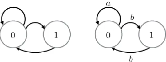
Example 2.4. ConsiderA11 ={0,1}andF ={11}and setX11 =XF. For every element
inX, there is no consequence 1. See Figure 2.2 for its graph representation.
0 1 0 1
a b
b
Figure 2.2: (left): The directed graph whose vertex shift is X11, (right): The labeled edge graph whose labeled edge shift is Xeven
2.2.2
Sofic shifts and factor maps
Let X, Y be subshifts. A map π : Y → X is σ-commute if σX ◦π = π ◦σY. A map
π : X →Y is a factor map if σ-commute and onto. The subshift X is called a factor of
Y. For (one-dimensional) subshifts every factor map can be represented by a block map [LM95, Theorem 6.2.9 (Curtis-Lyndon-Hedlund theorem)]. Consider alphabet setsAand
B. A map π : AN → B is called a block map with size N. A block map induces a shift
commuting map between AN and BN. Define π :AN →BN by
π({xn}) = {π(xnxn+1· · ·xn+N−1)}
for {xn}n∈N ∈AN. Observe that σBN ◦π =π◦σAN.
A subshift X is a soficshift if it is a factor of a subshift of finite type.
Example 2.5. ConsiderAeven ={a, b}andF ={ω ∈A∗ : no oddly consequentbappears inω}
and set Xeven = XF. Observe that Xeven is not of finite type. Define a block map π :A2
11→Aeven by
π(00) =a,π(01) =b and π(10) =b.
Then the image ofX11by the shift commuting mapπ induced byπ isXeven. HenceXeven
is sofic. See also Figure 2.2.
2.2.3
β
and
(
−
β
)
shifts
In this subsection we illustrate subshifts characterized by orders on full shifts. Important examples are β and (−β) shifts, which are not always sofic. Let A={0,1, . . . , p−1}. Definition 2.6 (lexicographical order). For x, y ∈ AN, x ≺ y if there exists i ≥ 0 such that xk =yk for every 0≤ k ≤i−1 and xi < yi. For x, y ∈AN, x≼y if either x=y or
x≺y. We call the order ≼ the lexicographical order.
Definition 2.7 (alternating (lexicographical) order). Forx, y ∈AN, x≺y if there exists
i ≥ 0 such that xk = yk for every 0 ≤ k ≤ i−1 and (−1)i(yi−xi) < 0. For x, y ∈ AN,
x≼yif eitherx=yorx≺y. We call the order≼the alternating (lexicographical) order. Consider the lexicographical or alternating order on AN. Take a maximal element a∈AN with regard to the order: σn(a)≼afor all n≥0. Set
Σa ={x∈AN:σn(x)≼a for every n≥0}.
Observe thatΣa is closed and shift invariant. By the definition,ω ∈L(Σa) if and only if ωi· · ·ω|ω|−1 ≼a0a1. . . a|ω|−i−1
for every 0≤i≤|ω|−1. For ω∈L(Σa) define
k(ω) =
%
max{k ≥1 :ω|ω|−k· · ·ω|ω|−1 =a0· · ·ak−1} if such k exists
0 else.
Set Fω ={x∈Σ
Lemma 2.8 ([SY, Lemma 4.1]). Take ω,ω′ ∈ L(Σa) such that k(ω) = k(ω′). Then Fω =Fω′
.
Let V ={k(ω) :ω∈L(Σa)} and consider it as a vertex set. Define an edge from i to j labeled by an alphabet a if there exists ω ∈L(Σa) such that ωa ∈L(Σa), k(ω) =i and k(ωa) =j. More precisely, in the lexicographical order case, there is an edge fromi toj
labeled byc if either of the following: • j =i+ 1 andc=ai;
• 0≤c≤ai−1, a0· · ·ai−1c∈L(Σa) and k(a0· · ·ai−1c) = j.
In the alternating order case, there is an edge from Vi to Vj labeled by c if either of the
following:
• j =i+ 1 andc=ai;
• when i is odd, ai+ 1≤c≤p−1,a0· · ·ai−1c∈L(Σa) and k(a0· · ·ai−1c) =j; • when i is even, 0≤c≤ai −1, a0· · ·ai−1c∈L(Σa) and k(a0· · ·ai−1c) =j
Denote by (G,φ) the labeled directed graph defined above. By the definition of (G,φ), we have
Σa ={x∈AN:x is an infinite labeled path on (G,φ)}.
Typical examples of subshifts represented by this way are β-shifts and (−β)-shift. A β-shift, which is introduced by Renyi [Re57], consists of β-expansions induced by a
β-transformationTβ : [0,1)→[0,1) defined by
Tβ(x) = βx− ⌊βx⌋
for everyx∈[0,1) where⌊ξ⌋ denotes the largest integer no more thanξ. Takeβ >1 and let b = min{n∈Z:β ≤n}. Define dβ,1 : [0,1)→{0,1, . . . , b−1} by
dβ,1(x) = ⌊βx⌋
for x ∈ [0,1). Then we get a sequence dβ(x) :={dβ,1(Tβnx)} for each x ∈ [0,1), which is
called the β-expansion of x. Let Σβ be the closure of {dβ(x) : x ∈ [0,1)}. Observe that
Σβ isσ-invariant. It is called theβ-shift. Letb= limx→1−0dβ(x). It is a maximal element
with regard to the lexicographical order and we have Σβ =Σb [Pa60].
A β-shift is of finite type if and only if b is finite: there existsn ≥1 such that bk = 0
for everyk≥n [Pa60]. Aβ-shift is sofic if and only ifbis eventually periodic: there exists
n ≥ 0 such that σn(b) is periodic [Bert86]. For every β > 1 the β-shift is topologically
A (−β)-shift, which is introduced by Ito and Sadahiro [IS09], consists of (−β)-expansions induced by (−β)-transformation T−β(0,1]→(0,1] by
T−β(x) = −βx+⌊βx⌋+ 1
for everyx∈(0,1]. This is not the original form by Ito and Sadahiro but the map defined above is topological conjugate with the original one. Take β > 1 and let b = ⌊β⌋+ 1. Defined−β,1 : (0,1]→{1, . . . , b} by
d−β,1(x) =⌊βx⌋+ 1
for x ∈ (0,1]. Then we get a sequence d−β(x) := {d−β,1(T−nβx)} for each x ∈ (0,1],
which is called the (−β)-expansion ofx. Let Σ−β be the closure of {d−β(x) : x∈(0,1]}.
Observe that Σ−β is σ-invariant. It is called the (−β)-shift. Let b = d−β(1), which is
a maximal element with regard to the alternating order. If b is not periodic with odd period, Σ−β =Σb and if b= (b1. . . bq)∞ with odd q,
Σ−β ={x∈{1, . . . , b}N : (1b1. . . bq−1(bq−1))∞ ≼σnx≼b for all n≥0}
[IS09]. A (−β)-shift is of finite type if b is periodic [FL09]. A (−β)-shift is sofic if b is eventually periodic [IS09].
We can easily find β > 1 for which the (−β)-shift is not transitive. The set of β
for which the (−β)-shift has the specification property is Lebesgue measure zero [Bu97]. However, the set is of full Housdorff dimension.
2.2.4
Dyck shifts
In this subsection we considerDyck shifts, for which the set of ergodic measures is arcwise-connected but not dense. Dyck shifts are first introduced by Krieger [Kr74] as an example of non-uniqueness of measure of maximal entropy. Dyck shifts are easy to understand by considering brackets. Alphabets are 2n symbols which consists of n pairs; each pair has left and right brackets. In the case of n = 2 we can write the four alphabets as (,[,],). The language of Dyck shifts are symbols in which the brackets are “opened and closed in the right order”: [()] is in the language but ((())] is not.
Let n ≥ 2. Set AL = {ak : 1 ≤ k ≤ n}, AR ={ak : 1 ≤ k ≤ n} and A =AL∪AR.
We regard an alphabet ak from AL as a left bracket and ak as the corresponding right
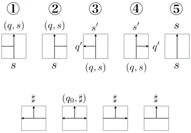
Define a transition function φ: (Σ∪{h})×A →Σ∪{h} by φ(u, v) = ⎧ ⎪ ⎪ ⎪ ⎪ ⎪ ⎪ ⎪ ⎪ ⎨ ⎪ ⎪ ⎪ ⎪ ⎪ ⎪ ⎪ ⎪ ⎩ uv if u∈(AL)∗ and v ∈AL, ε if u∈AL and v =u, h if u∈Am L, v ̸=um−1 where m≥1 u0· · ·um−2 if u∈AmL, v =um−1 where m≥2 v if u=ε, v ∈AL ε if u=ε, v ∈AR h if u=h.
We can extend it to the function Φ: (Σ∪{h})×A∗ →Σ∪{h} by
Φ(u, v0· · ·vm−1) =φ(φ(u, v0· · ·vm−2), vm−1)
for u∈Σ∪{h} and v0· · ·vm−1 ∈Am wherem ≥2. Define a forbidden setFD by
FD ={x∈A∗ : for every u∈Σ such that Φ(u, x) =h}
and define XFD by
XFD ={x∈AZ: there is no word from FD inx}.
Note that here we consider two-sided infinite sequences over A. Topology on AZ is the product topology of discrete topology. We consider the shift map extended to AZ in obvious way. (See also Appendix B.1).
Proposition 2.9 ([Cl]). The set Me of all ergodic measures of the Dyck shift is
arcwise-connected but is not dense in Me.
While essential parts of a proof are illustrated in [Cl], we try to give more precise proof.
Proof. Takex ∈XD. A bracket xi isclosed in x if it has the corresponding bracket in x:
there exists a subword ω0· · ·ωk−1 of xwhich includes xi such that Φ(ω0,ω1· · ·ωk−1) =ε. A bracket is open if it is not closed. We use the same terminologies with regards to a bracket in a wordx∈L(XD).
Let B− ⊂ X be the set of sequences where every left bracket is closed and B+ ⊂ X that of sequences where every right bracket is closed. First we show thatµ(B−∪B+) = 1 for every µ∈ Mσ(XD). For x ∈ XD let ℓ(x) = sup{i ∈Z : xi ∈ AL and it is open} and
r(x) = inf{i ∈ Z : xi ∈ AR and it is open}. Note that both ℓ(x) and r(x) is finite for
x∈XD \(B−∪B+). We can divide XD \(B−∪B+) into disjoint sets:
XD \(B−∪B+) = 0 i∈Z 0 j∈Z {x∈XD :l(x) =i, r(x) = j}.
Let Ai,j = {x ∈ XD : l(x) = i, r(x) = j}. Since σAi,j = Ai−1,j−1, we have µ(Ai,j) =
µ(A0,j−i) for every i, j ∈Z. Hence we can conclueµ(XD\(B−∪B+)) = 0. In particular,
we have µ(B−) = 1 orµ(B+) = 1 for every µ∈M
e(XD).
Let E(B−) be the set of ergodic measures on XD which gives probability one to
B−. Second we show that E(B−) is arcwise-connected. Set B = {0,1, . . . , n}. Define
ψ− :A→B by
ψ−(u) =
%
i if u=ai (∈AR),
0 if a∈AL
and let Ψ− : B− → BZ be the map induced by ψ
−, i.e. Ψ−({xk})ℓ = r−(xℓ) for every
{xk} ∈ B− and ℓ ∈ N. Let N ⊂ BZ be the set of sequences where infinitely many
consequent 0 appears. Since every left bracket is closed, the map Ψisσ-commute homeo-morphism from B− toBZ\N. The Dirac measure δ
0∞ is the only ergodic measure which
gives positive weight on N. Hence there is one-to-one correspondence between E(B−)
and Me(BZ)\ {δ0∞}. SinceMe(BZ) is arcwise-coneccted and we can avoid δ0∞, when we
connect ergodic measures in Me(BZ)\ {δ0∞}, E(B−) is arcwise-connected.
Similarly, we set E(B+) be the set of ergodic measures which gives probability one to
B+ and can show it is arcwise-connected. Since B−∩B+ ̸=∅, and we can easily find an ergodic measure in E(B−)∩E(B+), M
e(XD) is arcwise-connected.
Finally we show that Me(XD) is not dense inMT(XD). AssumeMe(XD) is dense in
MT(XD). Let ν = 12(δa∞
1 +δa2∞). For ε = 2−
11 take µ ∈ M
e such that d(µ,ν) < 2−11
wheredwill be defined in Section 3.2, which is compatible with the weak*-topology. Take a generic point x of µ. Then there exists N such that for every n≥N we have
1 n#{0≤k ≤n−1 :xk =a1}> 1 2 −2ε and 1 n#{0≤k ≤n−1 :xk=a2}> 1 2−2ε.
However there is no such a sequence in the Dyck shift. Taken ≥0 such that 210n ≥N. Looking at the first 210n alphabets in x, we have
#{0≤k ≤210n−1 :xk =a1}>511n, #{0≤k≤210n−1 :xk=a2}>511n
and the number of the other brackets is less than 2n. Considering left brackets which are open in x0· · ·x210n−1, we have
#{0≤k≤210n−1 :xk is a left bracket which is open in x0· · ·x210n−1}>509n. (2.1)
On the other hand, looking at the first 211n alphabets in x, we have
and the number of the other brackets are less than 4n. Hence we have
#{0≤k ≤211n−1 :xk is a right bracket which is open in x0· · ·x211n−1}>1018n
and
#{0≤k ≤211n−1 :x
k is a left bracket which is open in x0· · ·x211n−1}>1018n.
By the definition of Dyck shifts, no open left bracket exists at the left hand sides of any open right brackets: for ai ∈ AL and aj ∈ AR such that i ̸=j, if xki = ai and xkj = aj,
then kj < ki or there existsk ≥0 such thatki < k < kj and xk∈{ai, aj}. Therefore, the
right brackets which are open in x0· · ·x211n−1 should exist at the first 1030n alphabets,
i.e.
#{0≤k ≤1030n−1 :xk is a right bracket which is open in x0· · ·x211n−1}>1018n.
However (2.1) says that there are more than 509n open left brackets at the first 1024n alphabets. This is contradiction.
2.3
Invariant measures on symbolic systems
Throughout this section denote byΣp the full shift overA={0,1, . . . , p−1}. Recall that a σ-invariant measure is ergodic if µ(A) = 0 or µ(A) = 1 for every Borel set A such that
σ−1A=A. Simplest examples of invariant measure are periodic measures.
Example 2.10 (Periodic measure). Let x ∈ Σp be a periodic point with the smallest period n. A probability measure µdefined by
µ= 1 n n−1 ! k=0 δσkx
is called a periodic measure. It is easy to see that µ isσ-invariant and ergodic.
Forµ∈Mσ, define itssupportby supp (µ) =)C where the intersection is taken over
all closed sets with µ(C) = 1. The following examples are typical ergodic measures with full support.
Example 2.11 (Bernoulli measure). Define a probability measure µ′ on A by µ(i) = qi
for everyi∈A where+i∈Aqi = 1 andqi ≥0 for every i∈A. Then the product measure
µ on Σp is an ergodic σ-invariant Borel probability measure and is called a Bernoulli measure. Observe that if qi >0 for every i∈A, the Bernoulli measure has full support.
A generalization of Bernoulli measure is Markov measure, which is defined by using stochastic matrices. An n×n matrix P is a stochastic matrix if all its entries are non-negative and the sum of all entries for every row is one. A row vector q is a stationary probability vector for a stochastic matrixP if all its entriess are non-negative, the sum of all entries is one and satisfies qP =q. A non-negative matrix P isirreducible if for every
i, j there exists k ≥0 such that (Pk)
i,j >0. Note that by the Perron-Frobenius theorem
for an irreducible stochastic matrixP there exists a unique stationary probability vector
q all whose entries are positive [Ki98, Theorem 1.3.5]. A row vector is strictly positive if all its entries are positive.
Example 2.12 (Markov measure). Let P be a stochastic matrix andq = (q1, . . . , qp) be
a stationary probability vector for P. We define a Markov measure µ(q,P) as follows. For all cylinder sets of Σp define µ([k]) =qk for all alphabetsk and
µ([x0, x1, . . . , xm]) =qx0Px0,x1Px1,x2· · ·Pxm−1,xm
for all m ≥ 1, where Pk,l denotes the (k, l)-entries of P. Then this satisfies µ(∅) = 0
and σ-additivity on the algebra generated by the set of all cylinder sets. Hence it can be extended to a measure on Σp by the Carat´eodory extension theorem. Observe it is σ-invariant. We call theσ-invariant measure µ(q,P)aone-step Markov measure defined by the pair (q, P).
For a subshift of finite type X over A, let A be its adjacency matrix. Consider a stochastic matrix P such that for all i, j ∈A, Pi,j = 0 whenever Ai,j = 0. Then we can
obtain a Markov measure supported onX by the same way as above.
2.4
Coding
One way to understand dynamics of a system is create a topologically conjugate with a symbolic system. We start with an easy example of piecewise expanding Markov maps. LetX = [0,1 3,]∪[ 2 3,1],I0 = [0, 1 3] and I1 = [ 2 3,1]. Define f :X →[0,1] by f(x) = % 3x if x∈I0 3x−2 if x∈I1.
Obviously f is a piecewise expanding Markov map on X. Let Λ(f) = )n≥0f−nX. We
assign a 0,1 sequence to each x∈Λ(f) by coding its itinerary: define d:Λ(f)→{0,1}N by
d(x)i =j if fi(x)∈Ij (2.2)
for all x ∈ Λ(f) and i ∈ N. Observe that )n≥0f−nI
an is a singleton for every {an} ∈
d◦f = σ ◦d, which means (Λ(f), f) is topologically conjugate with the full shift over {0,1}. By this conjugacy we can interprets dynamics of (Λ(f), f) by infinite sequences over {0,1}.
The basic idea of this coding method is the following: we first divide a space into a finite regions, which we call a Markov parition. In the above case we choose a partition {I0, I1}. Second we track history of orbits and code their itinerary like (2.2). One thing we need to be careful is whether each sequence obtained by this coding corresponds to one point. Since f defined above is uniformly expanding, we can check it easily. For general piecewise expanding Markov maps, the condition (E2) ensures this point.
Other examples of this method are found in [KH95, Section 2.5, p.79], such as quadratic maps and Sinai’s horseshoe map. The existence of Markov partition is studied by many au-thors: for Hyperbolic toral automorphisms in [Berg67, AW67], for Anosov diffeomorphism in [Sin68], for pseudo-Anosov diffeomorphisms in [FS79] and for Axiom A diffeomorphisms in [Bow75] (See [Pe18] for more details).
Chapter 3
Structure of invariant measures and
convex functional technique
3.1
Borel probability measures
Let X be a compact metric space and B the Borel σ-algebra. Let C(X) be the Banach space of all continuous functions onX endowed with the supremum norm. The dual space
C(X)∗ of C(X) is the Banach space of all bounded linear functionals endowed with the
norm
∥F∥= sup{|F(φ)|:φ ∈C(X) with ∥φ∥= 1}. (3.1) LetM be the set of signed Borel measures on X and M1 be the set of Borel probability measures onX. Forµ∈Mits total variation|µ|is defined by|µ|(B) = sup+|µ(Bi)|for
every B ∈ B where the supremum runs over all partitions {Bi} of B. Set ∥µ∥ =|µ|(X)
and call it the total variation norm of µ
By Riesz’s representation theorem, there is a one-to-one correspondence betweenC(X)∗ and M in the sense that
Fµ(φ) =
$
φ dµ
for all φ∈ C(X). Moreover we have ∥Fµ∥ =∥µ∥. Throughout in this thesis, we use this
identification. Note that the set M1 is identified with
{F ∈C(X)∗ :F is positive and|F(1)|= 1}.
Recall that a bounded linear functionalF ∈C(X)∗ispositiveifF(φ)≥0 for allφ∈C(X) satisfying φ(x)≥0 for every x∈X.
In addition to (3.1) we consider the weak*-topology on M. The weak*-topology on M is the weakest topology which makes the map M∋ µ%→µ(φ)∈ R continuous for all
3.2
Simplex structure of invariant measures
Let (X, T) be a dynamical system where T is a continuous self-map on a compact metric space. Then MT is compact, metrizable and convex with regard to the weak*-topology.
Since C(X) is separable, there is a countable dense subset {fn}n∞=1 of C(X). For µ,ν ∈ MT define d(µ,ν) = ∞ ! n=1 |µ(fn)−ν(fn)| 2n∥f n∥ . (3.2)
Then it becomes a metric on MT and induces the weak*-topology. See [Wa82, Theorem
6.5] for compactness. Recall that a subset K⊂C(X)∗ isconvex if every convex
combina-tion of two points is contained inKwhere aconvex combinationofµ1, µ2, . . . , µn ∈C(X)∗
is the sum+nk=1akµk whereak ≥0 for allk = 1,2, . . . , nand+nk=1ak = 1. An elementµ
of a convex subset Kis not an extremal point if there exist ν1,ν2 ∈K \ {µ}and t∈(0,1) such that µ=tν1+ (1−t)ν2. We denote by ext(K) the set of extremal points of K. An extremal point of MT is ergodic i.e., ext(MT) =Me. ( See also [PU10].)
For µ ∈ MT there exists a unique Borel probability measure α on MT such that α(MT \ Me) = 0 and
µ(φ) =
$
Me
m(φ) dα(m)
for all φ∈ C(X) [PU10, Wa82]. We call α the disintegration of µ. For µ1, µ2 ∈ MT and
their disintegrations α1,α2, we have
∥µ1−µ2∥=∥α1−α2∥. (3.3) This equality plays an important role in the proof of Theorem A.
The unique integral representation and the equality (3.3) hold for more general set-tings. Let K be a non-empy compact metrizable convex susbset of C(X)∗ with regard to
the weak*-topology. Then the ext(K) is a Borel set [Ph01, Proposition 1.3]. An element
µ∈K is represented by a Borel probability measure α on K if
µ(φ) =
$
K
m(φ)dα(m) (3.4)
for allφ∈C(X). The setKis aChoquet simplexif eachµ∈Kis represented by a unique Borel probability measure α on K such that α(K \ext(K)) = 0. (See for more general definition [Ph01]).
From [Ru04, Appendix A.5] MT is a special case of the following. Let G be a closed
linear subspace of C(X)∗ such that µ ∈ G implies |µ| ∈ G. Then K = M(X)∩G is a
Choquet simplex. Moreover, forµ1, µ2 ∈Kand their decompositionsα1,α2 we have (3.3). In the case of invariant measures we putG ={µ∈C(X)∗ :T
3.3
The Bishop-Phelps theorem
In this section we prove the Bishop-Phelps theorem, following [I79, Theorem V.1.1]. It allows us to realize the perturbation in the space of continuous functions described in Introduction (see Figure 1.1). We show the Bishop-Phelps theorem in a general setting for the convenience of the reader. We begin with defining basic notions.
Definition 3.1. A functionalΓ:V →R on a Banach space V isconvex if
Γ(tφ+ (1−t)ψ)≤tΓ(φ) + (1−t)Γ(ψ) for all φ,ψ ∈V and t∈[0,1].
Let Γ : V → R be a convex and continuous functional on a Banach space V. A bounded linear functional F istangent toΓ atφ ∈V if
F(ψ)≤Γ(φ+ψ)−Γ(φ) (3.5) for all ψ ∈V.
A bounded linear functional F is boundedbyΓ if
F(ψ)≤Γ(ψ) for all ψ ∈V.
The dual space V∗ is a Banach space equipped with the norm
∥F∥= sup{|F(φ)|:φ ∈V with ∥φ∥= 1} (3.6) for all F ∈ V∗. We have reviewed that a Borel probability measure on a compact metric
space is identified with a bounded linear functional on the space of continuous functions which is positive and normalized. With this identification the notions of tangency and boundedness carry over to Borel probability measures.
The Bishop-Phelps theorem states that a Γ-bounded functional can be approximated byΓ-tangent ones with respect to the norm (3.6).
Theorem 3.2 ([I79, Theorem V.1.1.]). Let Γ : V → R be a convex and continuous functional on a Banach space V. For every bounded linear functional F0 bounded by Γ,
φ0 ∈ V and ε > 0, there exist a bounded linear functional F and φ˜ ∈ V such that F is
tangent to Γ at φ˜ and
∥F0−F∥ ≤ε and ∥φ0−φ˜∥ ≤ 1
ε(Γ(φ0)−F0(φ0) +s),
Proof of Theorem 3.2. Take φ0 ∈ V and ε > 0. Define Γ′(ψ) = Γ(ψ)−F0(ψ) +s for all
ψ ∈V wheres= sup{F0(ψ)−Γ(ψ) :ψ ∈V}. It is easy to seeΓ′ is continuous and convex. Let F′
0 = 0. Then F0′ is bounded by Γ′. and we have sup{F0′(ψ)−Γ′(ψ) : ψ ∈ V} = 0. Let ˜φ ∈V and F′ ∈V∗ which satisfy the conclusion for Γ′, φ0, ε and F0′. Then we have
∥φ0−φ˜∥ ≤ 1 εΓ ′(φ0) = 1 ε (Γ(φ0)−F0(φ0)−s) and F′(ψ)≤Γ′( ˜φ+ψ)−Γ′( ˜φ) =1Γ( ˜φ+ψ)−F0( ˜φ+ψ)−s2−1Γ( ˜φ)−F0( ˜φ)−s2 =Γ( ˜φ+ψ)−Γ( ˜φ)−F0(ψ)
for all ψ ∈V, which implies F0+F′ is tangent toΓ at ˜φ. Hence it is enough to show the case F0 = 0 and sup{F0(ψ)−Γ(ψ) :ψ ∈V}= 0.
For each φ ∈ V define C(φ) = {ψ ∈V :Γ(ψ)≤Γ(φ)−ε∥φ−ψ∥}. Observe C(φ) is closed and ψ ∈ C(φ) implies C(ψ) ⊂ C(φ). Take a sequence {φn}∞
n=0 of V such that
φn+1 ∈C(φn) and
Γ(φn+1)< ε
2n + inf{Γ(ψ) :ψ ∈C(φn)}.
Pick ψ ∈C(φn+1). By the choice of the sequence{φn}∞
n=0 we have Γ(φn+1)− ε 2n <Γ(ψ)≤Γ(φn+1)−ε∥φn+1−ψ∥ and ∥φn+1−ψ∥< 1 2n. (3.7) This implies {φn}∞
n=0 is a Cauchy sequence. Put ˜φ = limn→∞φn. Since C(φn) is closed,
˜
φ∈)n≥0C(φn). Moreover, the inequality (3.7) implies )n≥0C(φn) ={φ˜}. We have
Γ(ψ)≥0 for every ψ ∈V (3.8) because F0 = 0 is bounded by Γ. Since ˜φ∈C(φ0), we have
Γ( ˜φ)≤Γ(φ0)−ε∥φ0−φ˜∥. (3.9) By (3.8) and (3.9), we have
∥φ0−φ˜∥ ≤ 1
Define disjoint subsets
D={(ψ, y)∈V ×R:y <Γ( ˜φ)−ε∥φ˜−ψ∥}
and
E ={(ψ, y)∈V ×R:y ≥Γ(ψ)}.
ObserveDis open and convex andE is closed and convex. By the Hahn-Banach theorem there exists a continuous linear functional Λ:V ×R→R and t∈R such that
Λ(ψ, y)< t≤Λ(ψ′, y′) (3.10)
for all (ψ, y)∈D and (ψ′, y′)∈E. Define F(ψ) =−Λ(ψ,0) andL(y) = Λ(0, y). We may
assume L(y) = ky for some k ∈ R, since L is a linear map. The constant k is actually positive. Take y >Γ(φ0). By (3.8) and (3.9), we have
−y <−Γ(φ0)≤ −ε∥φ0−φ˜∥ ≤Γ( ˜φ)−ε∥φ0−φ˜∥. (3.11) Hence (φ0, y) ∈ E and (φ0,−y) ∈ D, which implies L(−y) < L(y). Since y is positive by (3.8), L is increasing and k > 0. Multiplying k−1, we may assume L(y) = y. Hence without loss of generality we may assume Λ is of the form Λ(ψ, y) =y−F(ψ).
Let ψ ∈V. By (3.10) we have sup (ψ,y)∈D y=Γ( ˜φ)−ε∥φ˜−ψ∥ ≤t+F(ψ)≤Γ(ψ) = inf (ψ,y)∈Ey. (3.12) Considering ψ = ˜φ, we have Γ( ˜φ)≤t+F( ˜φ)≤Γ( ˜φ). Hence t =Γ( ˜φ)−F( ˜φ). By (3.12) we have Γ( ˜φ)−ε∥φ˜−ψ∥ −F(ψ)≤Γ( ˜φ)−F( ˜φ)≤Γ(ψ)−F(ψ).
The first inequality gives
F( ˜φ)−F(ψ)≤ε∥φ˜−ψ∥
and the second inequality gives
Γ( ˜φ)−F( ˜φ) +F(ψ)≤Γ(ψ)
for all ψ ∈V. By considering ψ = ˜φ+ψ′ and ψ = ˜φ−ψ′ for arbitrary ψ′ ∈V, we have ∥F∥ ≤ε and F is tangent to Γat ˜φ. The proof is complete.
3.4
Uncountably many extremal points
Let X be a compact metric space and K be a Choquet simplex in C(X)∗. Define a
functionalQ:C(X)→Rby
Q(φ) = max{µ(φ) :µ∈K}.
Note that Q is continuous and convex. For φ ∈ C(X) an element µ ∈ K is maximizing
for φ ifQ(φ) = µ(φ). Denote byMmax(φ) the set of maximizing elements for φ. We show the existence of uncountably many maximizing extremal elements for a dense subset of continuous functions in this generalized setting. This section is dedicated to prove the following proposition.
Proposition 3.3 ([Sh17, Proposition 4.4]). Let K be a Choquet simplex in C(X)∗ such that the following holds.
(C1) for µ1, µ2 ∈K and their disintegrations α1,α2 we have ∥µ1−µ2∥=∥α1−α2∥; (C2) for µ ∈ ext(K) there exists a non-atomic Borel probability measure α on K such
that µ∈supp(α) and α(K \ext(K)) = 0.
Then there exists a dense subsetD of C(X) such that for every elementφ inD there exist uncountably many maximizing elements which are extremal points of K.
First we show that maximizing elements for φ are characterized by tangency to Q. This is proved by Br´emont in the case that K=MT [Br08, Lemma 2.3].
Proposition 3.4. For φ∈C(X)andµ∈C(X)∗, µ∈Mmax(φ)if and only ifµis tangent to Q at φ.
Proof. Let φ ∈C(X). By the definition of Q, µ∈ Mmax(φ) implies it is tangent to Q at
φ. We show the opposite direction. Take µ ∈ C(X)∗ which is tangent to Q at φ. For every ψ ∈C(X) we have
µ(ψ)≤Q(φ+ψ)−Q(φ)≤Q(ψ).
From [O07, Proposition 1.2.5] this impliesµ∈K. By using the inequality in the definition of tangency forψ =−φ, we have
µ(−φ)≤Q(φ−φ)−Q(φ) =−Q(φ).
Since µis linear, we have Q(φ)≤µ(φ). The proof is complete.
Second we consider the disintegration of a maximizing element for φ. The following proposition states that bounded liner functionals in the support of the disintegration of a maximizing element for φ are also maximizing forφ. The support of a disintegration α is defined by supp(α) =)C where the intersection is taken over all closed subsets C of K with α(C) = 1. Note thatα(supp(α)) = 1, since Khas a countable basis.
Proposition 3.5. Let µ∈ Mmax(φ) and let α be the disintegration of µ. Then supp(α)
is contained in Mmax(φ).
Proof. LetN ={ν ∈K:ν(φ)< µ(φ)}. Suppose α(N)>0. Then
µ(φ) = $ K m(φ) dα(m) = $ N m(φ) dα(m) + $ K\N m(φ) dα(m) <α(N)µ(φ) +α(K \N)µ(φ) =µ(φ).
This is a contradiction and then we haveα(N) = 0. SinceK \N =Mmax(φ) andMmax(φ) is closed, we have supp(α)⊂Mmax(φ).
Proof of Proposition 3.3. Note that every µ ∈K is bounded by Q. Pick φ0 ∈C(X) and 0 < ε < 1
2. Let µmax be a maximizing element for φ0. Without loss of generality we can assume µmax ∈ ext(K) by Proposition 3.5. Let ˜α be a non-atomic Borel probability measure on K for which (C2) holds with µmax. The continuity of ν %→ ν(φ0) and (C2) implies
˜
α3"µ∈ext(K) :Q(φ0)−ε2 ≤µ(φ0)
#4
>0. (3.13) Put Aε2 ={µ∈ ext(K) : Q(φ0)−ε2 ≤ µ(φ0)}. Denote by α0 the conditional measure of
α0 on Aε2, namely
α0(B) = 1 ˜
α(Aε2)α˜(Aε 2 ∩B)
for every Borel subset B of K. Note that α0(K \ext(K)) = 0. Let µ0 =
'
ext(K)m dα0(m). By applying Theorem 3.2 to φ0, µ0 and ε, there exist
φ∈C(X) and µ∈C(X)∗ such thatµ is tangent to Q atφ, ∥µ−µ0∥ ≤ε and ∥φ−φ0∥ ≤ 1 ε(Q(φ0)−µ0(φ0))≤ 1 εε 2 =ε.
Then φ is ε-close to φ0 and by Proposition 3.4 µis a maximizing element for φ.
Next we show the existence of uncountably many maximizing elements for φ which are extremal. Let α be the disintegration of µ and by (C1) we have
∥α−α0∥=∥µ−µ0∥ ≤ε. (3.14) Let ρ > 1−2ε > 0. Since α0 is a Borel probability measure and supp(α) is a closed set, there is an open set U such that supp(α) ⊂ U and α0(U \supp(α)) < ρ. Since K is a
metric space, there is a continuous function g :K→[0,1] which vanishes on K \U and is identically 1 on supp(α). Hence we have
α0(supp(α))>α0(U)−ρ≥
$
g dα0−ρ. The inequality in (3.14) implies
−ε≤
$
h dα−
$
h dα0 ≤ε for all h∈C(K) with ∥h∥= 1. Hence we have
α0(supp(α))> $ g dα0−ρ (3.15) ≥ $ g dα−ρ−ε ≥α(supp(α))−ρ−ε= 1−ρ−ε>0.
Since α0(supp(α)) = α0(ext(K)∩supp(α)) and α0 is non-atomic, supp(α) contains uncountably many extremal elements. By Proposition 3.5 we have supp(α) ⊂ Mmax(φ), and the proof is complete.
Chapter 4
Main theorems
Our main results are proved in this Chapter by following [Sh17] and [ST]. Using Propo-sition 3.3, we prove Theorems A and B. Then we show Theorem C by Theorem A and Realization Theorem.
4.1
Uncountably many maximizing measures
Recall Theorem A.
Theorem A ([Sh17, Theorem A]). Let (Σ,σ) be a topologically mixing subshift of finite type. There exists a dense subset D of C(Σ) such that for every φ in D there exist uncountably many ergodic maximizing measures with full support and positive entropy.
As we will see in Chapter 5, maximizing measures appear as zero temperature limit of equilibrium measures. In that context, it is interesting to pay attention to H¨older continuous functions in the dense subset D. The following corollary says such functions are cohomologous to constants.
Corollary 4.1 ([Sh17, Corollary]). Under the hypotheses of Theorem A, if φ in D is H¨older continuous, then there exists a continuous function u ∈ C(Σ) such that φ =
u−u◦σ+Q(φ).
We use Bousch’s result, which is called the Ma˜n´e-Conze-Guivarc’h lemma.
Theorem 4.2 ([Bou01, Th´eon`eme 1]). Suppose (X, T) is transitive and satisfing the weak expanding condition. For a continuous function f satisfying the Walters condition let Q(f) = maxµ∈MT
'
f dµ. Then there exists u∈C(X) such that for every y∈X u(y) =−Q(f) + max
T x=y(f+u)(x).
Proof of Corollary 4.1. First we reduce the proof to the case of Markov shifts. Assume that the consequence of Corollary 4.1 holds for every Markov shift. When we prove the above statement later, we only use the fact that φ has a maximizing measure with full support.
Let (Σ,σ) be a topologically mixing subshift of finite type. Since every subshift of finite type is topologically conjugate with a Markov shift, there exists a Markov shift (Σ′,σ) which is topologically conjugate with (Σ,σ) by a conjugacy mapΦ:Σ→Σ′. Take
φ ∈ D(Σ) which is H¨older continuous. Let φ′ = φ◦Φ−1. Since topologically conjugacy preserves support, φ′. has a maximzing measure with full support. Since φ′ is H¨older
continuous, we haveu′ ∈C(Σ′) such that φ′ =u′−u◦σ+Q(φ′). It is easy to check that
u=u′◦Φsatisfies φ=u−u◦σ+Q(φ).
Let (Σ,σ) be a Markov shift. Since a Markov shift satisfies the weak-expanding con-dition and a H¨older continuous function on a Markov shift satisfies the Walters concon-dition, we can use Theorem 4.2 (see also Appendix A). From Theorem 4.2 there exits u∈C(Σ) such thatu◦σ−u+Q(φ)≥φ. Writeφ =u◦σ−u+Q(φ)−r, wherer is continuous and satisfies r ≥ 0. We obtain ' φ dµ =Q(φ)−' r dν for all ν ∈ Mσ. Hence r ≥ 0 implies
µ ∈ Mmax(φ) if and only if supp(µ) ⊂ r−1{0}. Since φ has a maximizing measure with full support, r≡0.
In the proof of Theorem A we essentially use the simplex structure of Mσ and the
paths in Me constructed by Sigmund [Sig77]. The choice of these special paths enables
us to obtain properties of uncountably many ergodic maximizing measures. The strength of our proof is that we can control properties of uncountably many maximizing measures by choice of paths in Me. Losing information on support and entropy, we can use the
same recipe to get uncountably many maximising measures for more general systems. Let us say that Me is arcwise-connected if it is not a singleton and for every µ and ν ∈Me
such that µ ̸= ν there exists a homeomorphism [0,1] ∋ t %→ ft ∈ Me on its image such
that f0 =µ and f1 =ν.
Theorem B ([Sh17, Theorem B]). Let T be a continuous self-map of a compact metric space X. Suppose Me is arcwise-connected. There exists a dense subset D of C(X) such
that for every φ in D there exist uncountably many ergodic maximizing measures.
Recall Proposition 3.3.
Proposition 3.3 ([Sh17, Proposition 4.4]). Let K be a Choquet simplex in C(X)∗ such that the following holds.
(C1) for µ1, µ2 ∈K and their disintegrations α1,α2 we have ∥µ1−µ2∥=∥α1−α2∥; (C2) for µ ∈ ext(K) there exists a non-atomic Borel probability measure α on K such
Then there exists a dense subsetD of C(X) such that for every elementφ inD there exist uncountably many maximizing elements which are extremal points of K.
As we discussed in Section 3.2, MT is a Choquet simplex with (C1). In order to finish
the proof of Theorem B we construct a non-atomic measure on MT satisfying (C2).
Proof of Theorem B. Takeµ∈Me andν∈Me\{µ}. By the assumption, there exists an
arc f from µ toν. Let Leb[0,1] denote the Lebesgue measure on [0,1] and α =f∗Leb[0,1]. Then µ∈supp(α). Since f is a homeomorphism, the inverse image of a point in f([0,1]) is a singleton. Hence α is non-atomic. Since f([0,1])⊂Me, α(MT \ Me) = 0.
We see Sigmund’s result on paths between ergodic measures for subshift of finite type. For µ,ν ∈ Me a continuous function [0,1] ∋ t %→ ft ∈ Me which satisfies f0 = µ and
f1 =ν is called a path fromµ toν.
Theorem 4.3 ([Sig77]). Let (Σ,σ) be a topologically mixing subshift of finite type. Then for every µ,ν ∈Me there exists a pathf from µtoν with the following properties: (i) for
every measure m∈f([0,1]), f−1({m})is a countable set; (ii) every measure m∈f([0,1])
except for countably many ones is fully supported and has positive entropy.
Proof of Theorem A. Pickφ0 ∈C(Σ) and 0<ε< 12. We obtain a non-atomic Borel prob-ability measure on Me by modifying the proof of Theorem B. Let µbe a φ0-maximizing
measure and pick ν ∈ Me\ {µ}. Let f be a path from µ to ν for which the conclusion
of Theorem 4.3 holds. Since the inverse image of any point is countable, ˜α = f∗Leb[0,1] becomes non-atomic. By definition µ ∈ supp(˜α) and ˜α(Mσ \ Me) = 0. Then for ˜α the
inequality (3.13) holds.
Following the proof of Proposition 3.3, we define α0 to be the restriction of ˜α to the set Aε2 ={µ∈ Me :Q(φ0)−ε2 ≤µ(φ0)} and obtain φ ∈ C(Σ) and a Borel probability
measureα such that∥φ0−φ∥ ≤ε and supp(α)⊂Mmax(φ).
By Theorem 4.3, f([0,1]) contains uncountably many ergodic elements which are fully supported and have positive entropy. The definition of α0 impliesα0(Mσ\f([0,1])) = 0.
By (3.15) in the proof of Proposition 3.3 we have
α0(f([0,1])∩supp(α)) = α0(supp(α))>0.
Since α0 is non-atomic and f([0,1]) ⊂ Me, this implies f([0,1]) ∩ supp(α) contains
uncountably many ergodic elements which are fully supported and have positive entropy. By Proposition 3.5 we have
f([0,1])∩supp(α)⊂supp(α)⊂Mmax(φ) and the proof is complete.
4.2
Uncountably many Lyapunov maximizing
mea-sures
In this section we investigate Lyapunov maximizing measures for piecewise expanding Markov maps. Recall the definition of piecewise expanding Markov maps. Let p ≥2 be an integer and {αi}pi=0−1, {βi}pi=0−1 sequences in [0,1] such that
0 =α0 <β0 <α1 <β1 <α2 <· · ·<βp−1 = 1.
Put X =(pi=0−1[αi,βi]. A map f : X → [0,1] is a piecewise expanding Markov map onX
if it is a C1 map such that the following holds:
(E1) f maps each interval [αi,βi], i∈{0, . . . , p−1} diffeomorphically onto [0,1];
(E2) there exist constants) c > 0, λ > 1 such that for every n ≥ 1 and every x ∈
n−1
k=0f−k(X), |Dfn(x)|≥cλn.
Let E be the space of piecewise expanding Markov maps on X endowed with the C1 topology given by the norm
∥f∥C1 = sup
x∈X|
f(x)|+ sup
x∈X|
Df(x)|.
As we will see in Lemma 4.5, the spaceE is an open subset ofC1 functions onX. Since a non-empty open subset of a Baire space is also a Barite space,E becomes a (non-complete) Baire space.
For each f ∈E define
Λ(f) = *
n≥0
f−n(X).
Slightly abusing the notation, we denote by f the restriction of f to Λ(f).
As we illustrated in Section 2.4, (Λ(f), f) topologically conjugates with the full shift over p symbols. Let Σp = {0,1, . . . , p −1}N and πf : Σp → Λ(f) the topologically conjugacy defined by
{πf({ai}i≥0)}=
*
i≥0
f−i[αai,βai]
for every {ai}∈Σp. Theorem C is proved by combining Theorem A and the next lemma
which enables us to realize a perturbation inC(Σp) as a perturbation in E. Recall Theorem C.
Theorem C ([ST, Theorem A]). There exists a dense subset A of E such that the following holds for every f ∈A:
- χmin(f)̸=χmax(f);
- there exist uncountably many Lyapunov maximizing measures off which are ergodic, fully supported and have positive entropy;
- log|Df| is not H¨older continuous.
4.2.1
Proof of Theorem C
Lemma (the Realization Theorem). Letf0 ∈E be of classC2. For everyε>0 there exists a neighborhoodU of log|Df0|◦πf0 inC(Σp) such that for everyφ∈U there exists
f∞∈E such that
∥f0−f∞∥C1 ≤ε and log|Df∞|◦πf∞ =φ.
We finish the proof of Theorem C assuming the Realization Theorem.
Proof of Theorem C. Consider the dense subset Cσp of C(Σp) in Theorem A. Since C
2 maps are dense in E, the Realization Theorem implies that the set
5
A ={f ∈E: log|Df|◦πf ∈Cσp}
is dense in E. From Theorem A, if f ∈A5then there exist uncountable many Lyapunov maximizing measures which are ergodic, fully supported and have positive entropy.
LetE6denote the set of elements ofE for which there exist two periodic measures with different Lyapunov exponents. Clearly, iff ∈E6thenχmin(f)≠ χmax(f). SetA =A5∩E6. The set A satisfies the desired properties. Indeed, since E6is an open dense subset of E
and A5is a dense subset of E, A is a dense subset of E.
Let f ∈ A and suppose log|Df| is H¨older continuous. We use the result of Boush, Theorem 4.2 and derive a contradiction. The H¨older continuity of log|Df|and (E2) imply that log|Df| satisfies the Walters condition (See also Appendix A). Although (E2) does not imply the weak-expanding condition, (E2) implies that some iterate of f has this property: there exist an integer n ≥ 1 and λ > 1 such that |fn(x)−fn(y)| ≤ λ|x−y|
for all x, y in the same branch of fn. Since fn-invariant Borel probability measure is
weak*-approximated by periodic ones [Sig70], we have max
%$
log|Df| dµ:µ isfn-invariant
&
≤χmax(f).
By applying Theorem 4.2 to the map fn and the performance function −log|Df|, there exists a continuous function u such that
log|Df|≤u◦fn−u+ max
%$
log|Df| dµ:µis fn-invariant
&