Order of accuracy of numerical methods for fluid dynamics.

Vol.

9,

No.

2,

Juni

2014

Perancangan

Antena Mikrostrip Slot

untuk

Antena

Penerima

Sistem Televisi Digital

Adrian

Gulfyan

Putranto,

Aloysius

Adya

Pramudita-Penyelesaian

Analitik

Persamaan

Air

Dangkal

Pada Masalah Bendungan Bobol

Lusia Krismiyati Budiasih

Order of

Accuracy

of

Numerical Methods

for

Fluid

Dynamics

Sudi

Mungkasi

Penurunan Kandungan Minyak dan Lemak dalam

Air

Limbah

Menggunakan Perpaduan Proses

Elektrokoagulasi

dan

Adsorpsi

Sutanto,

Danang

Widjajanto

Pengenalan Nada Pianika Menggunakan Jendela Blackman

Dan

Ekstraksi

Giri

Transformasi

Fourier Gepat

Linggo.

Sumarno

Simulasi

Operasi

Logika

pada Dua Buah

Sinyal

Digital

Djoko

Untoro Suwarno,

KusminarTo,

Kuwat

Triyana

Efisiensi

Reduksi

Bunyi

Pada Penghalang

Bersusunan

Pagar

Dwiseno

Wihadi

Yogyakarta,

Juni 2014

tssN

1412

5641

Hlm.51-109

MediaTeknika

rssN

1412

5641

Editor in Chief

Associate Editors

Managing Editors

Administrator

Reviewers

Contact us

lssN

1412 5641

MediaTeknika

Volume

9

Nomor

2,

Juni

2014

Dr. lswanjono

Sudi Mungkasi, Ph.D.

Johanes Eka Priyatma, Ph.D. Dr. M. Linggo Sumarno

I Gusti Ketut Puja, M.T.

lwan Binanto, M.Cs.

Bernadeta Wuri Harini, M.T.

Catharina Maria Sri Wijayanti, S.Pd.

Dr. Hendra Gunawan Harno (Curtin University, Malaysia) Sudi Mungkasi, Ph.D. (USD)

Dr. Lidyasari (Unika Atma Jaya) Dr Iswanjono (USD)

I Gusti Ketut Puja, M.T. (USD) Dr. Pranowo (UAJY)

Media Teknika Journal Office Universitas Sanata Dharma Kampus

lll

Paingan Yogyakarta

Telp. (0274) 883037, 883986

ext.2310,2320

Fax. (0274) 886529

e-mail

: mediateknika@usd.ac.id

situs

: https://wrvw.usd.ac.id/lembaga/lppm

MediaTeknika

rs managed by Faculty of Science dan Technology, Sanata Dharma lJniversity for scientific

tssN 14125641

MediaTeknika

JurnalTeknologi

Vol.9, No.2,

2014

DAFTAR

ISI

perancangan Antena Mikrostrip Slot untuk Antena Penerima Sistem

Televisi

51-

58

Digital

Adrion Gulfon Putronto, Aloysius Adyo Pramudita

penyelesaian Analitik Persamaan Air Dangkal pada Masalah Bendungan

Bobol

59

-

70

Lusia Krismiyoti Budiosih

Order of Accuracy of Numerical Methods for Fluid

Dynamics

7t-76

SudiMungkosi

Penurunan Kandungan Minyak dan Lemak dalam Air Limbah

Menggunakan

77

-83

Perpaduan Proses Elektrokoagulasi dan Adsorpsi

Suto nto, Da na ng Widi oio nto

pengenalan _{Nada Pianika Menggunakan} Jendela Blackman dan

EkstrasiCiri

84-93

Transformasi Fourier CePat

Linggo Sumarno

simulasioperasiLogika pada Dua Buah

sinyalDigital

94-1OL

Djoko lJntoro Suworno, Kusminarto, Kuwot Triyona

Efisiensi Reduksi Bunyi pada Penghalang Bersusunan

pagar

102

-

109

iledlaTekn

i

ka

Jurnal Teknologi

Vol.9, No.2, Juni2014

.71

order

of

Accuracy

of

Numerical Methods

for

Fluid Dynamics

Sudi Mungkasi

Department of Mathematics, Faculty of Science _{and Technology, Sanata Dharma University,}

Mrican, Tromol pos 29, yogyakarta _{55002, lndonesia}

E-mail: sudi@usd.ac.id

Abstroct

This poper presents research results obout order of occurocy of numericol methods _{for fluid}

dynomics. High order occurote numerical methods are often desired. One could think that higher order

occurote numerical methods would olways leod to smoller numerical errors. However, this is misleoding.

A hiqh order occurote method does not meqn thot

it

is olways more accurote than a lower order

occurote method _for ony discretized domain. The truth of this cloim is demonstrated in this poper. We

consider _finite volume methods used to solve the shqllow woter equotions. These equotions _form a

mathemoticol model of _fluid dynomics governing shallow woter wqves or _{flows. Two} types of _finite

volume methods are implemented. The first is a _finite volume method which is second order occurate in

spoce _{but first} order dccurote in time. The second is a _finite volume method which

is

second order occurote in space as well as in time. One would hope that the second _finite volume method shoutd always produce smaller errors than the first. However, that is untrue, The _{first finite} volume method is

sometimes more accurqte thqn the second regordless of the quolity of the numericql solution.

Keywords: _finite volume methods, _fluid dynomics, order of accurocy, domain discretizotion

1. lntroduction

Some mathematical models for fluid flows are available in the literatures, such as the Saint-Venant model, the Boussinesq model, the Kortewig de Vries model, etc. To the author's knowledge, the most common in use for simulations of shallow water flows is the first, that is,

the

Saint-Venant _{model which was developed since 1892. This model is named after A.J.C.}

Barre de Saint-Venant (see the References _t1-7]).

The Saint-Venant model or as known as the shallow _{water equations can be used to} model and simulate flows in open channels. For example, we can simulate tsunami, flood, dam breaks, etc. using this model, as long as the flow or the wave is relatively shallow with respect

to the wave length. ln practice, researchers can now use either some software packages like ANUGA or Delf3D as an aid in the simulation, or code the numerical solver themselves.

A

well-known numerical solver

for the

shallow

water

equations

is

finite

volume method. This method is derived based on

the

integral equation rather than

the

differential equation of the model. Because _{integral equations do not need the assumption that solutions}

must be smooth, the finite volume method is able to handle smooth and nonsmooth solutions of the shallow water equations. This motivates the choice of finite volume method to be used

in

the

present paper, as

a

numerical method

in

interest. We use

the

Matlab programming

language to code the finite volume method of our work.

This paper shows that a lower order accurate method does not mean that

it

is always

less accurate than a higher order one in any condition. This claim was stated by LeVeque [g, 9]

without proof. We consider in this paper two types of finite volume methods

to

support the

truth

of this claim numerically. The

first

method is second order accurate in space but first order accurate in time. The second method is second order accurate in space and in time. We shall see that that the second method is actually less accurate in our simulations presented in

this paper.

72r

ISSN: 1412-5641

The rest of this paper is organized as follows. Section 2 provides the numerical method that we implement for simulations of water flows. Section 3 contains numerical results. Finally some concluding remarks are drawn in Section 4.

2. Research Method

ln this section we consider the one-dimensional shallow water equations that preserve

the steady state solutions to water motion. We refer to the work of Kurganov and Levy _[5] and

others [10, 11, L4-161for these equations. Assume

that

we are given a domain with space

variable

x

and time variable

l.

Both are free variables. We consider a bottom elevation given bV

B(r).

Water depth above the bottom is denoted by

h(x,t).

Water velocity is represented by

u(x,t).

We denote the free surface of water by

wi=

h + B

.ln

addition the acceleration due to gravity

is

g.

The one-dimensional shallow water equations

that

preserve

the

steady state solutions

to

water

motion are

then

given

by

the

following system

of two

simultaneous equations

w,

*

(hu)*

=0,

(hu\,

+l%

+

)s@

-u,'

].

=

-s(w

-

B)B.'

Again we refer to the work of Kurganov and Levy [K12002] for the discretization of equations (1) and (2).

It

is described as follows. We

first

consider the following general system

of

balance laws

(3)

e,*Y

*'

f

(q)

=

S(q,x,t)

where

xe

Rd

and

4€Rilsubject

to the initial condition

4(x,0)

= qo(x).We then take a

uniform cell-grid

x,

:

_{iLrc where}

Ax

is the cellwidth. The cellaverage

of

q(',t)

overthe

7 th cell is denoted bV

qiQ)

and is

| ***

(4)

Q 1(t)

::

:*[,",

r

q@,t)

&

. The system of balance laws can now be written

as

(5)

fia,at.

W

:

*f:

s(q(x,t),x,t)

&.

Further,

the

corresponding central-upw,rnd semi-discrete scheme

for the

system

of

balance laws

is

(G)

d

=

,,,

Hr.r,!D-H-,-rJ}-+S,(r),

*Ai\t)

Ar

,.

)'

with the numerical fluxes follows the formulation of Kurganov, Noelle and Petrova IKNP2001] and are given by

H,.,(t),=

W

.

**

(q.,.+

-

q,

-+).

-'i*i

-

i-i

t+i

t-i

Here q1*, :=

pi*r(xi*,,1)

and _ei*tr:=

pi(xr*rr,t)

are the right and the left values at the cell

interface

x

₌ X ,. , of a conservative non-oscillatory piecewise polynomial interpolant

l+i

q(x,t):)n/x,t)

x,.

I

(1) (2)

(71

illedlaTeknlka

Vol.9,

No.2, Juni 2014:

71-76

This polynomial interpolant is reconstructed

at

each

time

step from

the

previously computed cell averages,

{qiQ)}.

The notation

pr(.,t)

represents a polynomial of a specified

degree. The notation

y,

denotes

the

characteristic function over

the 7th

cell. ln addition, variables

aj*rare

the one-sided local speeds of wave propagation, which are determined by

oi.i

=

^*{^(#(r;)),^.(#*,.u,),

o},

(s)

,i*t:,"i,{a

(#r,.rr),0(#r,.,,),oi

(10)

discretizations of the source term.

Now coming back to the shallow water equations (1) and (2), we have

'

:l;,]'

r@)

=l%.!'r*-r,'],

s(q,*,')

:

[-

g(*0-

Du.f

(11)

Therefore, the one-sided local speeds ofwave propagation are

,,:*j=t

*t

,).+*

rfi,,ui*i+

rW,

o

.j,

$21

oi*i=mini

'i,

-

@,,ui*i-

rW,

o

.}'

(13)

Note that for our shallow water equations, a second _{order discretization of the} source term is

given by S---(')(/) = Q for the first component of the source vector and

ilediaTeknika

ISSN: 1412-5641

r73

for the second component of the source vector.

As in this paper we implement a second order finite volume method, a limiter is used

to suppress artificial oscillation in numerical solution. We use the minmod limiter

(14)

oi

=*nrn*(,#,L#)

(1s)

(16)

where

minmod(a,b)

::

j(s*f"l

+sgn(b))min(

a

l,

I b D.

This minmod limiter is implemented at every time step of _{the numerical evolution of finite}

volume methods.

3. NumericalResults

ln this section we provide a numerical demonstration for our claim that the method which is second order accurate in space and in time may actually less _{accurate than} the one

which is second order accurate in space but first order in time.

As a test case, we considera dam break problem with the spatial domain

-1<x<1.

lnitially

there is

dam

wall

at the point

x:0.

Note

that in this

paper

all

quantities are

measured in Systeme lntenational (Sl) units, so we omit the writings of units for simplicity. The

initial water depth on

the left of the wall

is

10,

while on

the

right

of the wall

is

4.

the

acceleration due to gravity is 9.81 .

74 I

ISSN:1412-5641

i

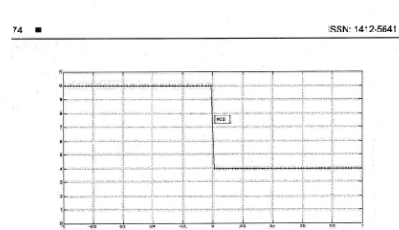
Figure 1. lnitial condition of water surface for the dam break problem at time / = 0.0 . Here the solid line

shows the analytical solution, whereas the dotted line shows the numerical solution using 100 cells.

Tabel 1. Numerical absolute .C errors for different numbers of

cells with second order in space and/irst order in time'

Number

of

Error of

cells

stage

Error of

discharge

Error of

velocity 100 200 400 800 1600

0.0478594

0,3738300

0,0243614

0,203973L

0.0109585

0.0868951

0.0053363

0.0425737

0.0026519

0,0215230

0.0600871

0.0296580

0.0135623 0.0055963 0.0032709

Tabel 2. Numerical absolute .C errors for different numbers of

cells with second order in space and second order in time. Number of

cells

Error of

stage

Error of

discharge

Error of

velocity 100 200 400 800 1600

0.0569322

0.4526225

0.0296662

0.2343232

0.0140053

0.1138955

0.0070051

0.0571872

0.0035362

0.0291737

0.0705843 0.0373933

0.0171898

0.0085543

o.0042862

As we run the simulations, absolute

D

errors are quantified at

time

I

=

0.05.

Those

errors are summarized in Table 1 and Table 2

for

various numbers

of

cells. Table 1 contains errors

for

different numbers

of

cells

with

second order in space and

first

order

in

time. ln

addition Table 2 presents errors

for

numbers of cells with second order in space and second

orderin time. Note that the analytical solution of this dam break problem has been derived by

Stoker[17] and extended

by MungkasilLz,13l.

This

test

case is also used by Goutal and

Maurel[3].

[image:7.584.56.498.38.293.2]

[image:8.612.6.598.19.821.2]

ilediaTeknika

ISSN: 1412-5641

Figure 2. Water surface for the breach of the dam at time I = 0.01, t = 0.04,1 _{= 0.08} . Here solid lines

show analytical solutions, whereas dotted lines show numerical solutions. The numerical solutions are

produced using the method which is second order in space and second order in time using 100 cells.

Slage ddambreat r.iet al I'me tso 025

75

I

0.6

o? o2

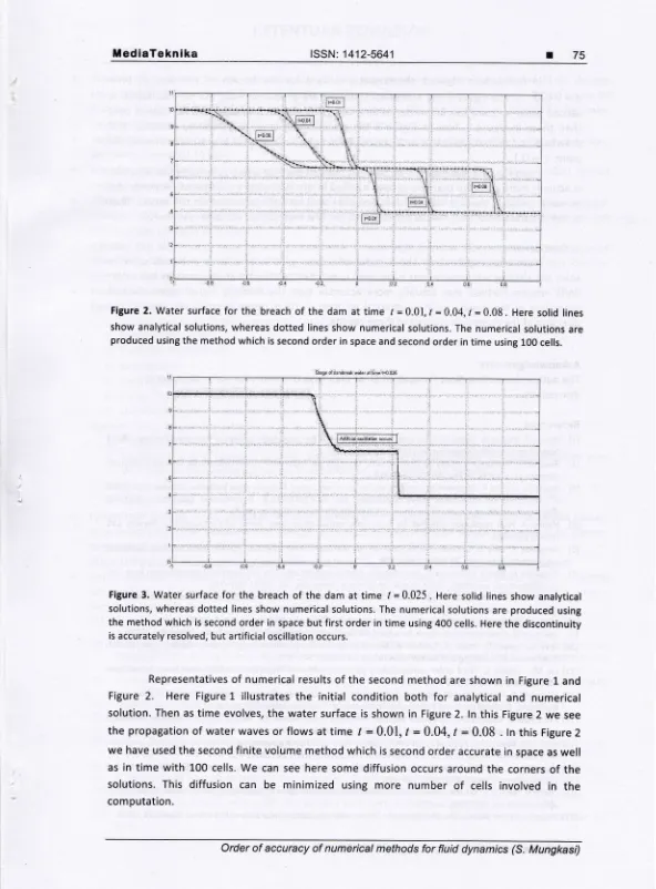
Figure 3. Water surface for the breach of the dam at time t =0.025. Here solid lines show analytical solutions, whereas dotted lines show numerical solutions. The numerical solutions are produced using

the method which is second order in space but first order in time using 400 cells. Here the discontinuity

is accurately resolved, but artificial oscillation occurs.

Representatives of numerical results of the second method are shown in Figure 1 and

Figure

2.

Here Figure

L

illustrates

the

initial

condition both

for

analytical and numerical solution. Then as time evolves, the water surface is shown in Figure 2. ln this Figure 2 we see

the propagation of water waves or flows at

time

I

:

0.01,

t :0.04, /

:

0.08 . ln this Figure 2

we have used the second finite volume method which is second order accurate in space as well as in time

with

100 cells. We can see here some diffusion occurs around the corners of the solutions. This diffusion

can

be

minimized using

more

number

of

cells involved

in

the computation.

76 I

ISSN:1412-5641

ln

comparison Figure

3

shows

water

surface

for the

breach

of the

dam

at

time

t =0.025.

ln this Figure3

the

numerical solutions are produced using

the

method which is

second order in space but first order in time using 400 cells. As we use more number of cells

than those

in

Figure 2, here

in

Figure 3

the

discontinuity is more accurately resolved. The

drawback of this method is that artificial oscillation occurs (see the water surface around the point

.r:

0

).

From Figure 2 and Figure 3 we see that the first method which is formally less accurate

is actually more accurate than the second method in the numerical experiments. However the minmod limiter in the first method does not work well, as artificial oscillation still occurs. That

is, the suppression of the artificial oscillation in the first method has not been successful.

4. Conctusion

Numerical experiments about order

of

accuracy

of finite

volume methods used to

solve the shallow water equations have been conducted. We find that the formally low.order

finite

volume method may actually more accurate than

the

formally higher order method regardless

of the

quality

of the

numerical solution. Further research could be taken in the direction of the numerical analysis of these results.

Acknowledgements

The author thanks Drs. Noor Hidayat, M.Si. of Brawijaya University for some stimulating

discussions.

I

References

111 Bianco F, puppo G, Russo G. High order central schemes for hyperbolic system of conservation laws, S/AM

Joarnol on Scientilic Computing, ?:L _{11999),294.322,}

fZt

Lir.frrr

F. Nonlineor sioiititi'ol finite volume methods for hyperbolic conservotion lows ond welbbalonced

schemes _for sources, Birkhauser, Bassel, 2004'

t3]

Goutal N, Maurel F., Momentum eqUation source term calculation & steady state validation, Proceedings of the

2'd Workshop on Dom-Break Wove Simulotion, No. HE-43/97/075/8, Deportement Loborotoire Notionol

d' Hydroulique, Groupe Hydraulique Fluviale, Eleetricite'de'France, Chatou, 1997'

t4]

Harten A. High resolution schemes for hyperbolic conservation laws. Jurnol of Computotionol Ph11sics, L35

ltgg7l,25b278.

151 Kurganov A, Levy D. Central-upwind schemes for the Saint-Venant system, ESAIM: Mathemoticql Modelling ond Numericol Anolysis,3S (2002),

397425.

l

16] Kurganov A, Noelle S, Petrova G. Semidiscrete centraFupwind schemes for hyperbolic conservation laws and

Hamilton-Jacobi equations. stAM Journol on scientific computing,23 (2001), 7O7-740.

171 Kurganov A, Tadmor E. New high-resolution central scheme for non-linier conservation laws and convection-diffusion equations, Jou rnal of Computqtionol Physics, 150.(2000), 247-282.

l8l

LeVeque RJ., Numerical methods _lor conservotion lows,znd Edition, Birkhauser, Basel, 1992.

t9l

LeVeque RJ, Finite-volume methods for hyperbolic problems, Cambridge University Press, Cambrid ge,2OO4.

[10] Levy D, Puppo G, Russo G. Central WENO schemes for hyperbolic systems of conservation laws, ESAIM:

Mothemtaticol Modelling and Numerical Anolysis,33 (1999), 547-571,

[11] Liu XD, Tadmor E. Third order nonoscillatory central scheme for hyperbolic conservation laws, Numerische

M oth e moti k, 79 (1998), 397 -425.

[12] Mungkasi S. A Study of well-balanced finite volume methods and refinement indicators for the shallow water equations, Thesis of Doctor of Philosophy, The Australian National University, Canberra, 2012.

[13] Mungkasi S, Roberts SG, Analytical solution involving shock waves for testing debris avalanche numerical

'

'

moOIts, Puie and Applied Geophysics, LGg (20121,187-1858.

[14] Naidoo R, Baboolal S. Application of the Kurganov-Levy semidiscrete numerical scheme to hyperbolic prOblems

with non-linear source tetm. Future Generation computer system,2o (2oo4l, 465473.

[15] Nessyahu H, Tadmor E. Non-oscillatory central differencing for hyperbolic conservation laws, Journol of Computational Physics, 87 (1990), 408-463.

[1G] Osher S, Tadmor E. On the convergence of difference approximation to scalar conservation laws, Mathemotics of Computotioa 5O (1988), 19-51.

[17] Stoker JJ. Woter Woves: The Mothematicol Theory with Application, lnterscience Publishers, New York, 1957.