T H E J O U R N A L O F H U M A N R E S O U R C E S • 45 • 2
Returns to Education
Alfonso Flores-Lagunes
Audrey Light
A B S T R A C T
Researchers often identify degree effects by including degree attainment (D) and years of schooling (S) in a wage model, yet the source of inde-pendent variation in these measures is not well understood. We argue that Sis negatively correlated with ability among degree-holders because the most able graduate the fastest, but positively correlated among dropouts because the most able benefit from increased schooling. Using NLSY79 data, we find support for this argument; our findings also suggest that highest grade completed is the preferred measure ofSfor dropouts, while age at school exit is a more informative measure for degree-holders.
I. Introduction
A central issue in labor economics is why credentialed workers (those with high school diplomas or college degrees) earn more than their non cre-dentialed counterparts. Such degree effects are consistent with sorting models of education (Arrow 1973; Spence 1973; Stiglitz 1975; Weiss 1983) in which employ-ers use credentials to identify workemploy-ers with desirable traits that cannot be directly observed.1Degree effects also are generated by human capital models (Becker 1964; Card 1995; Card 1999) if good learners are the ones who stay in school long enough to earn credentials, or if lumpiness in the learning process leads to more skill
ac-1. Following Weiss (1995), we use the term sorting to refer to both signaling and screening versions of the models.
Alfonso Flores-Lagunes is an assistant professor of food and resource economics at the University of Florida and a research fellow at IZA. Audrey Light is a professor of economics at Ohio State Univer-sity. The authors thank Lung-fei Lee and Ian Walker for useful discussions, Stephen Bronars for com-ments on an earlier draft, and Alex Shcherbakov for providing excellent research assistance. Alfonso Flores-Lagunes gratefully acknowledges financial support from the Industrial Relations Section at Princeton University. The data used in this article can be obtained beginning six months after publica-tion through three years hence from Audrey Light, Department of Economics, 410 Arps Hall, 1945 N. High Street, Columbus, OH 43210; light.20@osu.edu.
[Submitted August 2008; accepted February 2009]
quisition in degree years than in preceding years (Chiswick 1973; Lange and Topel 2006). Despite difficulties in distinguishing between these two competing models, the sorting versus human capital debate has dominated the degree effects literature for over 30 years.
Largely overlooked in this debate is the role of functional form in the interpre-tation of degree effects. In the earliest empirical studies (Taubman and Wales 1973; Hungerford and Solon 1987), degree effects were identified by including a nonlinear function of years of school (S) or categorical measures of degree attainment (D) in a log-wage model. More recently, analysts have taken advantage of richer survey data to implement a different identification strategy: Rather than includeS or Din their wage models, they control for both S and D (Frazis 1993; Jaeger and Page 1996; Arkes 1999; Park 1999; Ferrer and Riddell 2002). The interpretation of the resulting degree effects—defined as the wage gap between credentialed and non-credentialed workers conditional on years of schooling—is the focus of our analysis. When both S and D are included in a wage model, degree effects are identified because individuals with a given amount of schooling differ in their degree status or, stated differently, because years of schooling vary among individuals within a given degree category. We begin by considering how individuals’ schooling deci-sions could generate this variation inS and D. Among orthodox human capital and sorting models, only the sorting-cum-learning model of Weiss (1983) explains why
S and Dmight vary independently.2In Weiss’s model, individuals attend school for Syears and then take a test. High-ability individuals pass the test and earn a degree, while low-ability individuals terminate their schooling without a degree. While this behavioral framework justifies the inclusion of S and D in a wage model, it is inconsistent with the fact that individuals take varying amounts of time to earn identical degrees.
The empirical literature provides a number of explanations for why time to degree might vary across individuals. After documenting that the time typically needed to earn a college degree increased significantly between the 1970s and 1990s, Bound, Lovenheim, and Turner (2007); Bound and Turner (2007); and Turner (2004) con-sider such explanatory factors as declines in student preparedness as more high school graduates were drawn into college; corresponding declines in course avail-ability and other college resources that delay degree completion; and credit con-straints that led to increased in-school employment and enrollment interruptions among college students. Analyses of employment among high school and college students (Ruhm 1997; Light 1999; Oettinger 1999; Light 2001; Stinebrickner and Stinebrickner 2003; Parent 2006) and college transfer patterns (Hilmer 1997; Mc-Cormick and Carroll 1997; Hilmer 2000; Light and Strayer 2004) provide additional insights into why students vary in their time to degree completion.
To our knowledge, neither the theoretical nor empirical literature has considered a particular pattern that we find in the data: Wagesincrease with years of school (S) among both high school and college dropouts, but decrease in S among both
high school and college graduates. Given the lack of compelling explanations for the type of variation in S and D that would generate this particular pattern, we present a simple human capital model in which (i) individuals differ in ability; (ii) high-ability individuals acquire more skill than low-ability individuals during each year of school; (iii) degrees are awarded once a given skill threshold is reached; and (iv) lumpiness in learning causes individuals with varying ability levels to terminate their schooling upon crossing an identical degree threshold. In addition to predicting that high-ability individuals earn degrees and low-ability individuals do not, this model demonstrates how ability might be negatively correlated with time spent in school among degree holders: Everyone in this population reaches the same level of achievement, but the most able reach the threshold in the shortest time. Among individuals who do not earn a degree, however, those with the most ability stay in school the longest because they benefit from additional skill investments.
Our schooling model provides a rationale for including bothS and Din the log-wage function. Moreover, it leads us to specify a log-wage function in which theSslope varies across degree categories, and it predicts that theSslope is negative for degree holders and positive for nondegree holders. In contrast, earlier studies include in-dependent dummy variables for each degree category (D) and for schooling (S) (Frazis 1993; Jaeger and Page 1996; Arkes 1999; Park 1999; Ferrer and Riddell 2002), or they specify a fully interacted model with a dummy variable for everyS– Dcell (Jaeger and Page 1996; Park 1999). In the absence of an explicit theoretical justification for these functional forms, it is difficult to interpret the estimates.3
In estimating our log-wage model with data from the 1979 National Longitudinal Survey of Youth, we consider two additional issues. First, we acknowledge that the independent variation in S and D used for identification can arise from reporting errors as well as from the optimizing behavior described by our model. Because models that control for both S and D rely on variation in S within each degree category, the estimates are more vulnerable to noise than are estimates that rely on the total variation in the data. To contend with measurement error, we reestimate our wage equations withS and D data that are judged to be “clean” to determine whether seemingly error-ridden observations are driving our results. While misre-porting of bothS and Dhas been widely explored (Ashenfelter and Krueger 1994; Kane, Rouse, and Staiger 1999; Black, Berger, and Scott 2000; Bound, Brown, and Mathiowetz 2001; Flores-Lagunes and Light 2006), estimates from the “clean” sam-ple suggest that measurement error is not an important source of the independent variation inS and Dused to identify degree effects.
Second, we argue that the most common measure of years of school—namely, highest grade completed—is not always the preferred measure. For degree holders, we wish to know how long it takes to earn the credential. However, time to com-pletion is not fully captured by highest grade completed if the latter measures credits earned toward a degree—for example, high school graduates may report having
completed Grade 12 regardless of whether they earned their diploma in three, four, or five years. For this reason, age at school exit is our preferred measure of time spent in school for degree holders. Among dropouts, where our goal is to measure the skill acquisition that takes place prior to school exit, the opposite is true: Highest grade completed (that is, progress made toward a degree) is likely to be a better measure than age at school exit. In light of these concerns, we use both highest grade completed and age at school exit (conditional on work experience gained while in school) as alternative measures ofSin our wage models.
Our estimates reveal that the marginal effect ofSvaries across degree categories in the systematic manner predicted by our model: Each year ofSis associated with
higherwages among high school and college dropouts, and withlowerwages among high school and college graduates. For the two dropout categories, the positive slope is larger in magnitude (ranging from 0.02 to 0.05) and more precisely estimated whenSis measured as highest grade completed than whenSis measured as age at school exit. For the two degree categories, the negative estimates (ranging from
ⳮ0.002 toⳮ0.03) become much more precise when we measureSas age at school
exit rather than as highest grade completed. The independent variation inS and D
observed in the data appears to reflect important skill differences among individuals with a common degree status. By recasting degree effects as time in school effects conditional onD, we learn that dropouts who stay in school the longest are the most highly skilled of their type, as are graduates who complete their degrees in the shortest time.
II. Schooling Model
Our objective is to show why time spent in school (S) varies among individuals with a given degree status (D) and, in particular, why S is positively (negatively) correlated with ability among dropouts (graduates). We begin with a straightforward extension of Card’s (1995, 1999) formalization of Becker’s (1964) seminal model, in which individuals terminate their schooling when the marginal benefit equals the marginal cost. Becker (1964) and Card (1995, 1999) consider a single observed dimension—years of schooling (S)—in which to assess individuals: The moreSa worker has, the more skill and ability he is expected to embody. We augment this framework by assuming a degree is awarded to any individual who crosses a given skill threshold. We also assume that lumpiness in learning leads to a discontinuity in the human capital production function at the degree threshold. The discontinuity induces individuals with a range of abilities to terminate their schooling upon earning the degree—however, the more able among this group reach the thresh-old sooner than their less able counterparts because they acquire skill at a faster rate. Individuals who lack the ability to earn a degree never face the discontinuity, and instead make their schooling decision precisely as described in the Becker and Card models. Thus, dropouts exhibit the familiar pattern in which more able individuals stay in school longer than less able individuals.
rates and tastes. In addition, we assume that schools offer a single, identical degree and are essentially indistinguishable from one another—that is, we abstract from the role of school characteristics and programs of study in affecting how much a given individual will learn in a given amount of time. We make these simplifying as-sumptions in order to highlight the key features of our model. After presenting the model in Section IIA, we discuss in Section IIB the extent to which additional real world complexities might influence students’ schooling decisions.
A. Effects of Lumpiness in Learning on Schooling Decisions
We assume individual i chooses years of schooling (Si) to maximize the utility function
U
(
K,S)
⳱K(
S)
ⳮC(
S)
⳱g(
SA)
ⳮrS,(1) i i i i i i i
where Ki andAi represent individual-specific acquired skill and innate ability, re-spectively, and ris the discount rate. The function K(Si)⳱g(SiAi) is the human capital production function that describes how each additional year of school trans-lates into additional skill, andC(Si)⳱rSiis the associated cost function. In contrast to Card’s (1995, 1999) formulation we include skill, rather than earnings, as an argument in the utility function; the individual seeks to maximize the discounted, present value of skill which, along with ability, determines his postschool earnings.4
The substitution of Kifor earnings allows us to highlight the relationship between years of school and degree attainment, which we assume occurs whenever skill reaches the threshold KD. Following Card (1995, 1999), we assume skill increases withSat a decreasing rate, and that the marginal benefit ofSincreases inA. How-ever, we also assume that a discontinuity arises ing(SiAi) as the thresholdK
D is approached. This discontinuity only affects individuals whose ability is high enough to enable them to attain a degree, so we defer further discussion of this feature until we consider these individuals’ schooling decisions.
In Figure 1, we illustrate the schooling decisions of two individuals with relatively low levels of ability. Regardless of how long these individuals stay in school, their skill level does not get close enough to the thresholdKDfor lumpiness in learning to come into play. As a result, both individuals simply choose the schooling level at which the slope of their (continuous) production path equals the constant marginal cost r. For the individual with ability levelA1, this schooling level is S1; for his counterpart with the higher ability level A2, the optimal schooling level is S2. In short, individuals in this range of the ability distribution—all of whom leave school without degrees—exhibit the familiar pattern (Becker 1964; Card 1995; Card 1999) of positive correlation between ability, years of school, and skill.
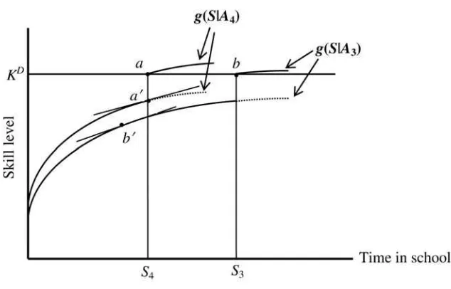
Next, we consider the schooling decisions of two individuals whose ability levels are sufficiently high to make degree attainment a possibility. Figure 2 shows that in the absence of any discontinuity, the individual with abilityA3finds his optimum at pointb⬘, while the individual with higher abilityA4choosesa⬘. As each individual
Time in school
Skill level
b
a
g
(
S
|
A
2)
g
(
S
|
A
1)
slope=
r
K
DS
1S
2Fig. 1
Time in school for low ability (A1) and high ability (A2) dropouts
Fig. 2
approaches skill threshold KD, however, his path shifts upward by a fixed amount. The upward shift in the production function (shown by the solid lines) is caused by lumpiness in learning—that is, individuals experience a contemporaneous increment in their skill level once they complete a program of study. This feature of the learning process was first suggested by Chiswick (1973) to explain how degree attainment could be associated with a larger wage increment than nondegree years in the ab-sence of job market signaling.
For the typeA4individual, the discontinuity shown in Figure 2 happens to occur
at the skill level associated withS4years of school, which is the point at which he would terminate his schooling in the absence of a discontinuity. The individual reaches an optimum (point a) on the higher path, and leaves schoolwitha degree afterS4years. The discontinuity induces the lower ability individual to move from
point b⬘ to point b (that is, to leave school with a degree after S3 years). More
generally, individuals in this ability range can choose to stay in school longer in order to exploit the benefits of lumpiness in learning, but the most able among them earn their degrees the fastest.
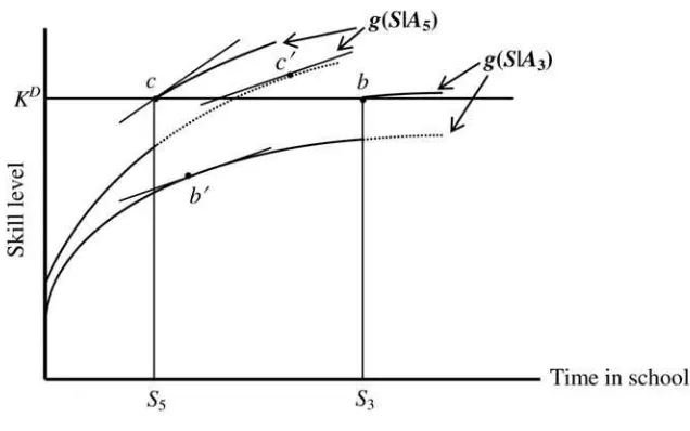
Thus far, we have assumed that lumpiness in learning produces a contempora-neous skill boost but does not affect the marginal cost or marginal benefit ofS. If the cost of continued schooling increases or tastes change once a degree is earned, then the discontinuity in the production function could be accompanied by an in-crease inr. If the productivity burst associated with degree completion is followed by a productivity slowdown, then the production function could not only shift up-ward but also flatten. Under either scenario (or a combination of the two), high-ability individuals might opt to leave schoolsoonerin response to the discontinuity. In Figure 3, we compare the typeA3individual from Figure 2 to an individual with ability A5 (which exceeds A4) under a scenario where marginal cost (r) increases
onceKDis reached. In the absence of a discontinuity or cost change, the individual with abilityA5would proceed beyond skill levelK
Dto pointc⬘.5If the upward shift
in his production path is accompanied by an increase inr, as shown in Figure 3, he chooses point c. In other words, he opts not to proceed beyond the degree. More generally, any increase in marginal cost or decrease in marginal benefit that accom-panies lumpiness in learning can cause typeA5individuals to join the typeA3and typeA4individuals in leaving school upon crossing the degree threshold. This leads
to even more variation in Samong individuals with identical degrees, while main-taining a negative relationship betweenSandA.
B. Additional Considerations
Our simple extension of Card’s (1995, 1999) schooling model demonstrates how particular patterns in the data might arise. While the pattern for dropouts (a positive relationship between S andA) emerges directly from the Card model, the reverse pattern for graduates is generated because we assume lumpiness in learning in
con-5. Pointc⬘in Figure 3 corresponds to staying in school beyond the single degree program that we assume is available. Clearly, we could extend our framework to include a higher degree, in which case the pro-duction function would contain another discontinuity at a skill level beyond KD
Fig. 3
Time in school for “higher” ability (A5) graduate who leaves school sooner in response to discontinuity
junction with the notion that degrees are awarded when a given skill level is reached. The notion thatS might represent something different for graduates than for drop-outs—and, as we demonstrate in Section V, the fact that the dropout-graduate con-trast holds at both the high school and college level—appears not to have been analyzed elsewhere in the literature.
The literature has extensively explored the broader issue of why time in school and time to degree (especiallycollegedegree) vary across individuals. Becker (1964) and Card (1995, 1999) describe precisely how factors affecting both marginal benefit and marginal cost affect a given individual’s schooling attainment. Bound, Loven-heim, and Turner (2007); Bound and Turner (2007); and Turner (2004) consider a range of factors to explain why the timing of college degree attainment slowed during the 1970s and 1980s. Research on the employment of high school and college students (Ruhm 1997; Light 1999; Oettinger 1999; Light 2001; Stinebrickner and Stinebrickner 2003; Parent 2006) and college transfer patterns (Hilmer 1997; Mc-Cormick and Carroll 1997; Hilmer 2000; Light and Strayer 2004) provide additional explanations for why years of school would vary across students. An exhaustive exploration of whySwould vary among individuals in a given degree/dropout cate-gory is beyond the scope of this study, but we consider a subset of issues that are potentially relevant to the interpretation of our findings.
are related to labor market productivity. The key issue for our analysis is that fi-nancially constrained students are the most likely to accumulate in-school employ-ment experience, which has been shown in some studies (Ruhm 1997; Light 2001) to have a direct effect on postschool earnings. Thus, variation inSamong individuals with a given degree status might reflect not only variation in ability, as assumed by our model, but variation in in-school experience as well. In estimating our wage models, we include detailed measures of both in-school and postschool work ex-perience. This enables us to assess the (degree-specific) effect of S on log-wages net of the effect of work experience.
By assuming that skill (KD) is identical among degree holders, we also abstract from the fact that school characteristics and programs of study can affect how much is learned, conditional on student ability or time spent in school; an extensive lit-erature explores the effects of school quality and college major on subsequent earn-ings (Brewer, Eide, and Ehrenberg 1999; Dale and Krueger 2002; Arcidiacono 2004; Altonji, Elder, and Taber 2005). A related issue is that college quality can affectS
if, for example, students at resource-constrained colleges are forced to delay their degree completion because of enrollment limits in courses needed to graduate. This phenomenon is shown by Bound, Lovenheim, and Turner (2007) and Bound and Turner (2007) to be an important determinant of secular increases in time to college degree completion, and it can potentially affect cross-sectional variation inSas well. Of course, resource squeezes on some college campuses cannot explain variation in
Samong high school graduates as well as college graduates, nor can it explain why
Sis wage enhancing among college dropouts. Nonetheless, we acknowledge that for college graduates, S can be negatively correlated with college quality as well as individual ability.
Our theoretical framework also makes the simplifying assumption that individuals face no uncertainty about their own abilities. Although this assumption is imposed more often than not in the schooling literature, uncertainty is worth discussing be-cause it has been invoked by Chiswick (1973) and Lange and Topel (2006) to explain how degree effects could arise in the absence of job market signaling or lumpiness in skill acquisition. The argument is that individuals discover their true ability over time, and that the least able drop out of school in response to this discovery while the more able—who learn more than the less able duringeveryyear of school—remain in school to complete the degree. We acknowledge that individ-uals may discover their true ability while in school and that the degree effects that we estimate in Section V might reflect this type of selection-on-ability in addition to lumpiness in learning.6 However, neither of these existing studies helps us
un-derstand whyS and D vary independently, or why the relationship betweenSand ability differs for graduates and dropouts.
III. Econometric strategy
In Section II, we assumed that each individual chooses his years of school (S) to maximize acquired skill (K) which, in conjunction with innate ability (A), determines his postschool starting wage. Employers cannot observeK and A
directly, but they can observe degree status andS. Thus, the prediction that emerges from our theoretical model is that wages increase with Samong dropouts and de-crease with Samong graduates, because Sis associated with higher ability among dropouts and lower ability among graduates.
To assess this prediction, we specify a wage function that allows log-wages to evolve with experience, and schooling attainment to affect the intercept (but not the experience slope) of the experience-earnings path (Mincer 1974). Our theoretical discussion calls for a functional form that allows the intercept of the log-wage path to increase with each successive degree category and to change with years of school-ing within each category. Thus, we specify the followschool-ing wage function:
4 4
Y⳱ ␣D Ⳮ ␦D SⳭZⳭu,
(2) i
兺
k ki兺
k ki i i ik⳱1 k⳱1
whereYiis the natural logarithm of the average hourly wage for individuali,Dkiis a vector of dummy variables identifying degree categories,Siis time in school,Zi is a vector of additional covariates (cumulative labor market experience and its square and dummies identifying race and gender), and ui represents unobserved factors. In contrast to the simplifying assumption made in Section II that workers earn a single degree upon reaching a given skill threshold, we now allow for two successive degrees. Specifically,Dkdistinguishes between high school dropouts (D1),
high school graduates (D2), college dropouts (D3), and college graduates (D4).7Our
model predicts that log-wages increase monotonically with each successive degree (␣1␣2␣3␣4), and that the effect ofS on these degree effects is positive for
dropouts (␦10,␦30) and negative for degree holders (␦20,␦40).
It is worth reiterating that our specification is not generally used in the degree effects literature. The orthodox approach—often dictated by a lack of independent data onS and D—is to use a spline function or step function inSand omit separate measures ofD(Hungerford and Solon 1987; Belman and Heywood 1991). Among studies that control for bothS and D, most include degree dummies and an inde-pendent (noninteracted) function of S (Frazis 1993; Jaeger and Page 1996; Arkes 1999; Park 1999; Ferrer and Riddell 2002). This is equivalent to imposing the re-striction␦
1⳱␦2⳱␦3⳱␦4, although some studies relax our restriction thatYis a linear
function of S. Jaeger and Page (1996) and Park (1999) propose alternative specifi-cations that allow for interactions between S and D, but they use an extremely flexible functional form that includes a parameter for every year-of-schooling/degree combination. We propose Equation 2 as the most parsimonious way to capture the
D–S-specific intercepts that are consistent with our schooling model.
Our goal is not to identify the causal effect of schooling on log-wages, but to assess the signs of the degree-specific schooling slopes unconditional on innate abil-ity. As long as S, DandZare known to employers and are reasonable proxies for productivity, we can use ordinary least squares (OLS) to estimated the parameters in Equation 2. While we maintain these assumptions, we cannot assume that our survey data are reported without error. Unfortunately, the instrumental variables and generalized method of moments estimators that are often used to account for mea-surement error inS or D(Ashenfelter and Krueger 1994; Kane, Rouse, and Staiger 1999; Black, Berger, and Scott 2000; Flores-Lagunes and Light 2006) are inappro-priate for our application because they allow only one covariate to be reported with error, and they require two, independent reports for the error-ridden variable.8In the
absence of a tractable estimation strategy that accounts for measurement error in both S and D, we compare estimates from our primary sample to those from an alternative sample of seemingly “clean” responses to determine whether our results are sensitive to the inclusion of seemingly erroneous data.9
The notation used in Equation 2 implies that we use cross-sectional data for estimation and, in fact, a cross-section composed of each individual’s postschool starting wage is our primary sample. We also use a panel sample consisting of annual wages reported by each sample member from school exit to the end of the obser-vation period. Regardless of which sample is used, we fit thesame lifecycle wage path and identify thesame S–D-specific intercepts; the “all wages” sample simply adds observations beyond the first year (or so) of experience, and potentially en-hances the precision of all parameter estimates. However, a disadvantage of the “all wages” sample is that estimates of ␣
k and␦k will be biased if unobserved factors affecting later wages (for example, employer learning and/or on-the-job training) are related to S and D. We present estimates based on the “all wages” sample for comparison, but prefer the cross-sectional sample of starting wages. We use ordinary least squares to estimate the models with both samples, but when using the panel (“all wages”) sample we correct the standard errors for nonindependence across observations for a given worker. All models are estimated after transforming the data into deviations from sample-specific grand means. We describe each sample in Section IV.
IV. Data
A. Sample Selection and Variable Definitions
We use data from the 1979 National Longitudinal Survey of Youth (NLSY79) to estimate the wage functions described in Section III. The NLSY79 began in 1979
8. We have an independent report of high school graduation status for a subset of respondents for whom high school transcripts were collected, but the NLSY79 does not provide similar validation data for college attendance and degrees. Similarly, we have sibling-reported highest grade completed for respondents with in-sample siblings, but these reports predate final schooling attainment for many respondents.
with a sample of 12,686 youth born in 1957–64, and it remains in progress today. Respondents were interviewed annually from 1979 to 1994 and biennially thereafter; 2004 is the last year for which data were available when we carried out the analysis. The NLSY79 is an ideal source of data for our analysis because respondents report their highest grade completed, dates of enrollment, and degree attainment; the survey also provides unusually detailed information on labor market activities, which en-ables us to net out the potentially confounding effects of work experience gained while in school.
The first step in our data creation process is to identify each respondent’s chro-nological sequence of diplomas and degrees received, along with the date when each credential was awarded. If an individual attended high school, college, or graduate school without earning a diploma or degree, we include his attendance spell and dropout date in the degree sequence. To construct this sequence, we use the follow-ing self-reported information: (i) whether the respondent holds a high school diploma or has passed the general educational development test (GED) at the date of the interview and, if so, the month and year of diploma/GED attainment; (ii) whether the respondent is enrolled in school at the time of the interview and, if not, the month and year of his last enrollment; (iii) the respondent’s enrollment status in every month since the last interview; (iv) the month/year the respondent last attended his first, second, and third most recent colleges; and (v) the type and month/year of receipt of as many as three diplomas and degrees or, in earlier survey years, of the highest degree.10 When identical diplomas or degrees are reported multiple times, we generally use the first-reported date; we resort to subsequently reported dates or to the enrollment timelines when information is missing.
We use this information to place each respondent into one of five categories: high school dropout, high school graduate, college dropout, college graduate (bachelor’s degree recipient) or graduate degree recipient. Those respondents who complete their schooling without interruption are classified according to their final degree or drop-out status. When individuals receive their schooling discontinuously, we assign them the dropout/degree status that prevails the first time they leave school for at least 18 months. Only 6 percent of respondents change their degree status between this 18-month school exit and their last school exit, so our estimates are not affected by which school exit date is used as long as we control for work experience gained during the interim. We are limited in our ability to form postbachelor’s degree categories because our theoretical model assumes that individuals holding a given degree are homogeneous with respect to acquired skill, and we lack the sample size to define separate categories for holders of master’s, professional, and doctoral de-grees. In addition, we are unable to identify the degree programs being pursued by graduate school dropouts. Thus, we combine all graduate degree holders—who make up 2.7 percent of the sample—into a single category (D5), but we do not include interactions betweenD5andSin our wage model. Graduate school dropouts remain in our sample as college graduates if they are nonenrolled for at least 18 months
between college and graduate school, and report a wage during the interim. As we demonstrate in Section V, our findings are unaffected by whether we categorize graduate students in this fashion, or eliminate them from the sample altogether; additional, unreported experiments, such as moving graduate school dropouts into a sixth category and adding interactions betweenS and the postcollege degree cate-gories also proved not to affect our inferences.
We choose not to segment the college dropout category into two-year college dropouts, two-year college graduates, and four-year college dropouts because these groups are conceptually indistinct, given the frequent use of two-year colleges as stepping stones to four-year colleges (Rouse 1995; Hilmer 1997; Light and Strayer 2004). For example, we would hesitate to argue that a student who earns an asso-ciate’s degree in two years and then spends one year at a four-year college differs in ability from a student who enrolls at a four-year college for three years. We substantiate this decision in Section V by demonstrating that eliminating two-year degree holders from the sample does not significantly affect our estimates. We also show that our inferences do not depend on whether we treat individuals with a GED as high school dropouts (our default classification) or high school graduates.
After classifying each sample member with respect to highest degree, the second step in our data creation process is to identify the corresponding years of school. During each interview, respondents are asked to report their current highest grade completed if they have attended school since the last interview. We use the value reported during the first interview after the degree or dropout date as one measure of time in school, which we now refer to asS1. As an alternative measure of time in school, we use the degree or dropout date in conjunction with the respondent’s birth date to determine the age (measured to the nearest month) at which he or she left school; we refer to this variable asS2.
The degree or dropout date used to defineS2 also serves as the career start date. With this date in hand, the next step in our data creation process is to select alter-native samples of postschool wages. Our cross-sectional starting wage sample uses the first wage reported after the degree is awarded or the individual drops out of school. Our “all wages” sample includes that same wage, plus a maximum of one wage per year reported by the individual over the remainder of the panel, which ends when he reenrolls in school or is last observed. Given our strategy of allowing the intercept of the age-earning profile to depend on an individual’sS–D combina-tion, each wage sample has its own advantage. The “all wages” sample provides more data with which to fit the log-wage path. The starting wage sample contains relatively little variation in postschool work experience, which minimizes the pos-sibility thatDandSare correlated with unmeasured components of work experience due, perhaps, to the most able workers investing more intensively in on-the-job training than less able workers.
history information available in the NLSY79 to construct a measure of cumulative weeks worked from the eighteenth birthday to the date when the wage is earned. In addition, we use the work experience reported by 16- and 17-year-olds (available for respondents who are younger than 18 when the survey begins) to compute av-erage work effort at age 16–17 as a fraction of work effort at age 18, by sex, race/ ethnicity, and degree status. We then use these averages to assign every sample member a measure of predicted, early experience. We control for actual experience since age 18 and its square, along with predicted early (younger than age 18) ex-perience in each of our wage models.
Our starting wage sample consists of a single observation for each of 11,712 individuals. While the original NLSY79 sample has 12,686 respondents, we elimi-nate 313 individuals for whom degree status, degree/dropout dates, and/or highest grade completed cannot be determined. We eliminate another 661 individuals be-cause a postschool wage is not reported. The “all wages” sample contains between one and 21 observations for the same 11,712 individuals, for a total of 126,019 observations.
In addition to analyzing the entire starting wage sample of 11,712 individuals, we also examine a subsample in which schooling and degree variables are judged to be “clean.” To construct this subsample, we exploit the fact that degree attainment and highest grade completed (S1) should conform to certain institutional norms if re-spondents consider their progress toward a degree when reporting their highest grade completed. We expect high school dropouts to complete grade 11 or lower, high school graduates to complete grade 12, college dropouts to complete at least grade 12 but less than grade 16, and college graduates to complete grade 16. In forming a “clean” sample, we eliminate individuals if their reported S1–D combination is sufficiently far from these expectations: We requireS1ⱕ12,S1⳱11–13, S1⳱12–
16,S1⳱15–19, andS1ⱖ16 for individuals in the high school dropout, high school
graduate, college dropout, college graduate, and graduate degree categories, respec-tively. This strategy eliminates roughly 3 percent of observations in each high school and college category, and 1.3 percent of the graduate degree holders. The remaining sample consists of 11,277 individuals for whom theS1 and D data are invariably less error-ridden than the data in the larger sample. By comparing estimates for our two samples, we can assess the effect of measurement error on the estimates.11We
do not construct a similar “clean” sample using our alternative variableS2 (age at school exit) because parttime and discontinuous enrollment often delay school exit. We control for these delays by including detailed experience measures in our wage model, but we lack clear expectations of the unconditional relationship between age at school exit and degree attainment.
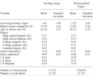
B. Summary Statistics
Table 1 reports summary statistics for the variables used to estimate wage models for both the starting wage and “all wages” samples. Table 2 contains a
Table 1
Summary Statistics for Selected Variables
Starting wages All postschool
wages
Variable Mean Standard
deviation
Mean Standard
deviation
Ln(average hourly wage) 1.81 1.09 2.23 2.02
Highest grade completed (S1) 12.49 2.44 12.40 2.36
Age at school exit (S2) 21.10 5.13 20.12 3.70
Degree
High school dropout (D1) 0.17 0.17
High school diploma (D2) 0.33 0.37
College dropout (D3) 0.34 0.32
College graduate (D4) 0.13 0.13
Graduate degree (D5) 0.03 0.01
Actual experiencea 2.74 4.02 9.21 6.88
Early experienceb 0.07 0.23 0.08 0.27
1 if male 0.51 0.53
1 if black 0.25 0.27
1 if Hispanic 0.16 0.18
Number of observations 11,712 126,019
Number of individuals 11,712 11,712
a. Hours worked from eighteenth birthday to date wage was earned, divided by 2,000. b. Hours worked between sixteenth and eighteenth birthday
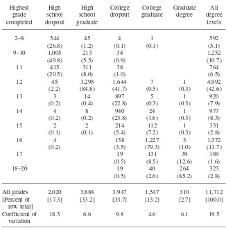
lation of highest grade completed (S1) and degree status (D). It is clear from these distributions that S1 varies considerably within D category. A comparison of the coefficient of variation across columns reveals that S1 varies far more within each dropout category than within each degree category; this conforms to the notion that
Table 2
Highest Grade Completed by Highest Degree Received
Highest
All grades 2,020 3,888 3,947 1,547 310 11,712 [Percent of
row total]
[17.3] [33.2] [33.7] [13.2] [2.7] [100.0]
Coefficient of variation
18.3 6.6 9.8 4.6 6.1 19.5
Note: The table shows the number of sample members reporting each S–D combination. Percents of column totals are in parentheses.
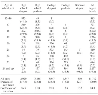
clear that this alternative measure of time in school varies far more within degree category than does highest grade completed. While there is no expected age at which individuals complete each degree category, given that school exit dates can be ex-tended by parttime or interrupted enrollment, it is interesting to note that only 86 percent of high school dropouts leave school by age 18, only 53 percent of high school graduates earn their degrees at age 18, and only 32 percent of college gradu-ates earn their degrees at age 22. In short, age at school exit diverges fromS1Ⳮ6
Table 3
Age at School Exit by Highest Degree Received
Age at
All ages 2,020 3,888 3,947 1,547 310 11,712 [Percent of
row total]
[17.3] [33.2] [33.7] [13.2] [2.7] [100.0]
Coefficient of variation
16.5 11.8 21.8 13.9 16.2 24.3
Note: The table shows the number of sample members reporting eachS–Dcombination. Percents of column totals are in parentheses.
V. Findings
Table 4 presents estimates of the degree-specific intercepts (␣
k) and
D–S interaction terms (␦k) for a variety of wage model specifications, all of which
use highest grade completed (S1) as our measure of time in school; additional pa-rameter estimates for each specification are in Table A1. We discuss these estimates before turning to the corresponding estimates in Tables 5 and A1 in which S1 is replaced with age at school exit (S2).
The
Journal
of
Human
Resources
Table 4
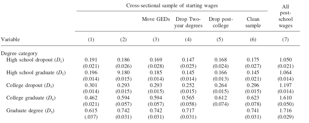
OLS Estimates of Alternative Wage Models Using Highest Grade Completed as Measure of Time in School
Cross-sectional sample of starting wages All
post-school wages Move GEDs Drop
Two-year degrees
Drop post-college
Clean sample
Variable (1) (2) (3) (4) (5) (6) (7)
Degree category
High school dropout (D1) 0.191 0.186 0.169 0.147 0.168 0.175 1.050
(0.021) (0.026) (0.028) (0.025) (0.024) (0.027) (0.021)
High school graduate (D2) 0.196 9.180 0.185 0.145 0.166 0.145 1.064
(0.014) (0.015) (0.014) (0.014) (0.013) (0.021) (0.014)
College dropout (D3) 0.301 0.293 0.293 0.252 0.264 0.296 1.197
(0.014) (0.015) (0.015) (0.015) (0.015) (0.015) (0.014)
College graduate (D4) 0.462 0.594 0.594 0.565 0.612 0.623 1.610
(0.021) (0.057) (0.057) (0.058) (0.074) (0.078) (0.050)
Graduate degree (D5) 0.615 0.742 0.742 0.717 0.741 1.716
Flores-Lagunes
and
Light
457
S1 interacted with
High school dropout (D1) 0.019 0.016 0.020 0.020 0.016 0.028
(0.006) (0.006) (0.006) (0.006) (0.006) (0.005)
High school graduate (D2) ⳮ0.002 0.006 ⳮ0.002 ⳮ0.002 ⳮ0.012 ⳮ0.014
(0.009) (0.007) (0.009) (0.009) (0.026) (0.007)
College dropout (D3) 0.039 0.039 0.028 0.040 0.040 0.053
(0.006) (0.006) (0.007) (0.006) (0.007) (0.005)
College graduate (D4) ⳮ0.015 ⳮ0.015 ⳮ0.016 ⳮ0.014 ⳮ0.028 ⳮ0.023
(0.015) (0.015) (0.015) (0.018) (0.022) (0.013)
Number of observations 11,712 11,712 11,712 10,900 10,999 11,277 126,019
Note: Column 3 moves GED recipients from categoryD1toD2. Column 4 omits two-year degree recipients from categoryD3. Column 5 omits graduate school dropouts
from categoryD4and all graduate degree recipients. Column 6 omits observations with highly implausible S–D combinations (see text for details). Column 7 uses annual
The
Journal
of
Human
Resources
Table 5
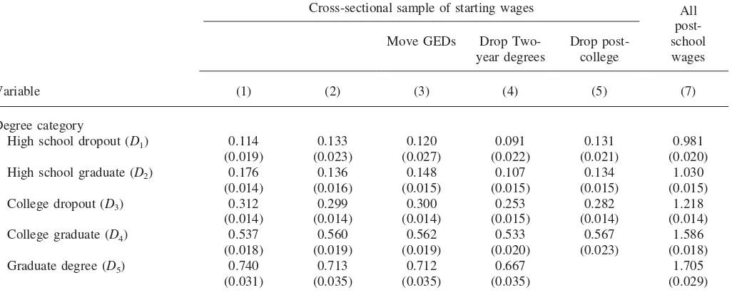
OLS Estimates of Alternative Wage Models Using Age at School Exit as Measure of Time in School
Cross-sectional sample of starting wages All
post-school wages Move GEDs Drop
Two-year degrees
Drop post-college
Variable (1) (2) (3) (4) (5) (7)
Degree category
High school dropout (D1) 0.114 0.133 0.120 0.091 0.131 0.981
(0.019) (0.023) (0.027) (0.022) (0.021) (0.020)
High school graduate (D2) 0.176 0.136 0.148 0.107 0.134 1.030
(0.014) (0.016) (0.015) (0.015) (0.015) (0.015)
College dropout (D3) 0.312 0.299 0.300 0.253 0.282 1.218
(0.014) (0.014) (0.014) (0.015) (0.014) (0.014)
College graduate (D4) 0.537 0.560 0.562 0.533 0.567 1.586
(0.018) (0.019) (0.019) (0.020) (0.023) (0.018)
Graduate degree (D5) 0.740 0.713 0.712 0.667 1.705
Flores-Lagunes
and
Light
459
S2 interacted with
High school dropout (D1) 0.003 0.001 0.002 0.006 0.009
(0.004) (0.005) (0.004) (0.004) (0.005)
High school graduate (D2) ⳮ0.019 ⳮ0.013 ⳮ0.019 ⳮ0.017 ⳮ0.023
(0.003) (0.003) (0.003) (0.003) (0.003)
College dropout (D3) 0.002 0.002 ⳮ0.001 0.006 0.001
(0.002) (0.002) (0.002) (0.002) (0.001)
College graduate (D4) ⳮ0.010 ⳮ0.010 ⳮ0.011 ⳮ0.013 ⳮ0.024
(0.003) (0.003) (0.003) (0.003) (0.003)
Number of observations 11,712 11,712 11,712 10,900 10,999 126,019
Note: Column 3 moves GED recipients from categoryD1toD2. Column 4 omits two-year degree recipients from categoryD3. Column 5 omits graduate school dropouts
from categoryD4and all graduate degree recipients. Column 6 uses annual wage observations reported from school exit to the observation period’s end; standard errors
effects conditional onS1. Based on the Column 1 estimates, we would predict that the gap in log wages between high school graduates and high school dropouts is 0.005 (0.196–0.191), the corresponding gap among college graduates and dropouts is 0.16 (0.462–0.301), and an additional year of school is associated with a 2 percent wage boost for all workers.12When we allow the relationship betweenS1 and log
wages to vary across degree categories (Column 2), we estimate a much larger college degree effect than what is seen in Column 1 (0.30 versus 0.16), and we reject at a 1 percent significance level the null hypothesis that the estimated S1 effects are equal across degree categories.
Moreover, the estimates in Column 2 provide support for our theoretical argument that wages increase (decrease) with time in school among dropouts (graduates). The estimated D–S coefficients are 0.019 and 0.039 for the high school and college dropout categories, respectively, and an imprecisely estimatedⳮ0.002 andⳮ0.015
for the corresponding graduates categories. These point estimates are consistent with the notion that time in school is positively correlated with ability for dropouts but negatively correlated with ability for degree holders. For the two degree categories, the imprecision of the estimated interaction terms is consistent with the evidence (Table 2) thatS1 varies less for graduates than for dropouts. Although the existing variation produces parameter estimates with the predicted signs, we believe highest grade completed is not the preferred measure of time in school for degree holders. In Columns 3–5 of Table 4, we assess the effects on our OLS estimates of re-classifying certain degree types. In Column 3, we move GED recipients from the high school dropout category to the high school graduate category. This increases the predicted log-wage gap associated with earning a high school degree but has relatively little effect on the estimated interaction effects. The estimated coefficient for the interaction betweenS1 andD2 reverses sign, but continues to be statistically insignificant. In Column 4, we eliminate two-year degree holders from the sample rather than include them in the college dropout category. Eliminating these relatively high wage earners leads to a decrease in the estimated S1 coefficient for college dropouts, but does not qualitatively affect our findings. In Column 5, we eliminate individuals with postcollege schooling from the sample. Again, this does not alter our inferences regarding the estimated effects ofS1 within each degree category.
Our next task is to assess the effects of measurement error on our estimates. In Column 6 of Table 4, we report estimates based on a “clean” sample that excludes observations where the reportedS–D combination is highly implausible (for exam-ple, no high school diploma butS1⳱16, orS1⳱12 and a bachelor’s degree). The
differences between these estimates and the corresponding estimates in Column 2 are not significantly different from zero. Despite the fact that the standard errors increase (as expected) when we switch to the clean sample, the estimatedS1 coef-ficients associated with the two degree categories actually become larger in absolute value. The “clean” estimates are consistent with the predictions of our model and with the notion that measurement error inS and Dis relatively unimportant.
The final column of estimates in Table 4 is based on our “all wages” sample. We maintain our original degree classifications and include seemingly error-ridden ob-servations in this sample, so the Column 7 estimates should be compared to the estimates shown in Column 2. Qualitatively, the Column 7 estimates substantiate the evidence seen in Column 2: Predicted log-wages increase with each successive degree category and increase (decrease) with each additional year of school for dropouts (graduates). Quantitatively, all four estimated coefficients for the S1–D
interactions are slightly larger in absolute value when we use the “all wages” sample than when we rely on the cross-sectional sample, although the college dropout cate-gory is the only one for which we reject the null hypothesis of pair-wise equality across models.13This comparison suggests thatSmight be weakly, positively
cor-related with unobserved factors that increase log-wages as the career unfolds. Such a correlation could arise for at least two reasons. First, although we assume em-ployers useDandSto discern worker productivity at the outset of the career, they may not completely learn their workers’ true abilities for a few years, at which point they further reward the high-S (high ability) individuals. Altonji and Pierret (2001) and Lange (2007) provide evidence of this form of employer learning. Second,
high-S (high ability) workers might gain work experience that is not captured by our cumulative experience variable, or simply receive higher returns to on-the-job train-ing. Because we do not allow the experience paths to differ across S–D categories, such fanning out on the basis of ability would be subsumed by our estimated inter-cepts. In general, however, a switch to the “all wages” sample produces only minor changes to the point estimates, and does not significantly affect our key findings.
Next, we ask how our estimates change when we replace highest grade completed (S1) with age at school exit (S2) as our measure of time in school. Table 5 contains estimates for wage models that use this alternative measure, but are otherwise iden-tical to the corresponding specifications in Columns 1–5 and 7 of Table 4; the Column 6 estimates are omitted from Table 5 because we lack priors on the uncon-ditional relationship between degree and age at school exit needed to select a “clean” sample.
In comparing the estimates shown in Columns 1 and 2 of Table 5, we again reject at a 1 percent significance level the equal slope restriction imposed by Specification 1. Using the preferred Specification 2, we find that replacing highest grade completed with age at school exit has little effect on the estimated degree effects, although we now predict a slightly larger wage gap between college dropouts and high school graduates than what is seen in Table 4. However, switching schooling measures has a significant effect on the estimated coefficients for theS–Dinteractions. In Column 2 of Table 4, we saw that the estimatedS1 coefficient is positive (and significant) for dropouts and negative (but insignificant) for graduates. The parameter estimates have the same signs in Table 5, but now the estimated coefficients for both dropout categories are essentially zero (0.002–0.003 with standard errors at least as large as the parameter estimates) while the estimated coefficients for the two degree cate-gories are precisely estimated and, in the case of high school graduates, larger in
absolute value (ⳮ0.019 versus ⳮ0.002 in Table 4).14 The estimates change very
little when we reclassify GED recipients as high school graduates (Column 3), elim-inate two-year degree holders (Column 4), or drop individuals with postcollege schooling (Column 5). When we switch to the “all wages” sample (Specification 7), the estimated effect ofS2 continues to be zero for the two dropout categories, but becomes larger in absolute value for the two degree categories—although, using conventional significance levels, we reject the null hypothesis of equality across models for the college graduate category only.
To understand why our estimates are sensitive to the manner in which we measure time in school, it is useful to consider the two degree categories (high school and college graduates) separately from the two dropout categories. Even if holders of a given degree do not have identical levels of acquired skill, as assumed by our theoretical model, they complete similar programs and earn a similar number of credits. Consider one individual who earns a high school diploma at age 18, and another who earns the same diploma a year earlier. Both should report their highest grade completed as 12 to reflect the fact that they completed the final year of their program, but their reported school exit dates should differ because one of them completed the program more quickly than the other. In short, age at school exit is a more informative measure of what we wish to know about degree recipients— namely, the speed with which they complete a common grade or degree program. Therefore, it comes as no surprise that the estimatedS2 slopes in Table 5 (based on age at school exit) predict that degree holders earn approximately 2 percent less (for high school graduates) and 1–2 percent less (for college graduates) for every extra year they take to graduate, whereas the corresponding estimates in Table 4 (based on highest grade completed) lack statistical significance.
In contrast, we believe highest grade completed is a more informative measure than age at school exit for both dropout categories. Our goal is to measure the amount of school completed (that is, credits earned) in order to control for hetero-geneity in skill among individuals with a given nondegree status. If reported accu-rately, highest grade completed is likely to be the preferred measure of schooling attainment for this purpose, given that future dropouts may “drag out” the time to school exit by failing courses, being truant, and otherwise spending time neither learning nor acquiring work experience. We believe the estimated slope coefficients in Table 4, which imply that high school (college) dropouts earn 2–3 percent (3–5 percent) more for every year spent in school, are preferred for assessing the effects of time spent in school among these individuals.
We can offer additional evidence to substantiate the argument that age at school exit is the preferred measure for degree holders in the sense that it measures (inverse) innate ability, whereas highest grade completed is the preferred measure of skill and ability among dropouts. In 1980, over 90 percent of NLSY79 respondents completed the Armed Services Vocational Aptitude Battery (ASVAB). NLSY79 users have access not only to individual ASVAB scores, but also to scores for the Armed Forces
Qualification Test (AFQT), which are computed from respondents’ scores on four parts of the ASVAB (word knowledge, paragraph comprehension, arithmetic rea-soning, and mathematics knowledge). Because AFQT scores are considered to be good measures of premarket skills (Neal and Johnson 1996), we assess their cor-relation with both measures of time spent in school for each degree-specific subsam-ple.15Among individuals in both degree categories, age-adjusted AFQT scores are strongly, negatively correlated with age at school exit but not with highest grade completed. Within both dropout categories, age-adjusted AFQT scores are strongly, positively correlated with highest grade completed, whereas the correlations with age at school exit are small and negative for college school dropouts and zero for high school dropouts.
VI. Concluding Comments
Our analysis begins with the observation that researchers often iden-tify degree effects by controlling for both degree attainment (D) and years of school-ing (S) in a wage model without considering why these two measures of schooling attainment would vary independently. We argue that individuals with a given degree are roughly homogenous with respect to acquired skill, but because the more able can earn their degrees relatively quickly,Sis negatively correlated with innate ability among this population. Conversely, individuals who drop out of a given degree program vary considerably with respect to both innate ability and acquired skill, and
S is positively correlated with these traits. Our simple extension of Card’s (1995, 1999) schooling model justifies the inclusion of bothDandSin a wage model, and suggests that the effect of schooling on log-wages should be allowed to differ across degree categories.
In estimating wage models that control for bothDandSusing data from the 1979 National Longitudinal Survey of Youth, we identify a number of patterns that are consistent with our model. First, we find that the data resoundingly reject the re-striction that the effect of years of school on log-wages is equal across degree categories—in other words, it is important to include degree dummies (D) andS–D
interactions, rather than simply controlling forS and D. Second, our estimates in-dicate that additional time in school is associated with higher wages for high school dropouts and college dropouts, but with lower wages for high school graduates and college graduates. Third, schooling effects for the two dropout categories are esti-mated more precisely when we use highest grade completed as the measure of S
than when we use age at school exit. For the two graduate categories, the opposite is true. Fourth, our estimates prove to be largely invariant to our attempts to account for measurement error in self-reportedS and D, which suggests that the independent variation in these two dimensions of schooling attainment is not dominated by “noise.”
The fact that our alternative measures of time spent in school (age at school exit and highest grade completed) appear to capture different information for degree holders and dropouts is a useful finding in its own right. We argue that high school and college graduates are expected to complete grades 12 and 16, respectively, and that, as a result, the age at which they earn their degrees is a more informative measure of ability than is their highest grade completed. Conversely, highest grade completed is a useful measure of progress made toward a degree among dropouts, whereas variation in age at school exit might reflect time spent neither gaining work experience (which we are able to control for separately) nor learning. Our estimates suggest that individuals within a given degree or dropout category vary considerably with respect to their ability and/or acquired skill, and that additional measures of schooling attainment are useful for explaining variation in postschool wages. While ours is not the first study to view schooling attainment as a multidimensional con-struct, we suspect there is far more to be learned by exploring heterogeneity in completion patterns among individuals with a given level of schooling attainment.
References
Altonji, Joseph G., Todd E. Elder, and Christopher R. Taber. 2005. “Selection on Observed and Unobserved Variables: Assessing the Effectiveness of Catholic Schools.”Journal of Political Economy113(1):151–84.
Altonji, Joseph G., and Charles R. Pierret. 2001. “Employer Learning and Statistical Discrimination.”Quarterly Journal of Economics116(1):313–50.
Arcidiacono, Peter. 2004. “Ability Sorting and the Returns to College Major.”Journal of Econometrics121(1):343–75.
Arkes, Jeremy. 1999. “What Do Educational Credentials Signal and Why Do Employers Value Credentials?”Economics of Education Review18(1):133–41.
Arrow, Kenneth J. 1973. “Higher Education as a Filter.”Journal of Public Economics 2(3):193–216.
Ashenfelter, Orley, and Alan Krueger. 1994. “Estimates of the Economic Returns to Schooling from a New Sample of Twins.”American Economic Review84(5):1157–73. Becker, Gary. 1964.Human Capital; a Theoretical and Empirical Analysis, with Special
Reference to Education. New York: Columbia University Press (for the National Bureau of Economic Research).
Belman, Dale, and John S. Heywood. 1991. “Sheepskin Effects in the Returns to Education: An Examination of Women and Minorities.”Review of Economics and Statistics 73(4):720–24.
Black, Dan A., Mark C. Berger, and Frank A. Scott. 2000. “Bounding Parameter Estimates with Nonclassical Measurement Error.”Journal of the American Statistical Association 95(451):739–48.
Bound, John, Charles Brown, and Nancy Mathiowetz. 2001. “Measurement Error in Survey Data.” InHandbook of Econometrics, Volume 5, ed. James J. Heckman and Edward E. Leamer, 3705–843. Amsterdam: Elsevier Science.
Bound, John, Michael F. Lovenheim, and Sarah Turner. 2007. “Understanding the Increased Time to the Baccalaureate Degree.”Research Report 07–626, Population Studies Center. Ann Arbor: University of Michigan.
Brewer, Dominic J., Eric R. Eide, and Ronald G. Ehrenberg. 1999. “Does It Pay to Attend an Elite Private College? Cross-Cohort Evidence on the Effects of College Type on Earnings.”Journal of Human Resources34(1):104–23.
Card, David. 1995. “Earnings, Schooling, and Ability Revisited.” InResearch in Labor Economics, Volume 14, ed. Solomon Polachek, 23–48. Greenwich, Conn.: JAI Press. ———. 1999. “The Causal Effect of Education on Earnings.” InHandbook of Labor
Economics, Volume 3, ed. Orley Ashenfelter and David Card, 1801–63. Amsterdam: Elsevier Science B.V.
Chiswick, Barry. 1973. “Schooling, Screening, and Income.” InDoes College Matter? Some Evidence on the Impact of Higher Education, ed. Lewis C. Solomon and Paul J. Taubman, 151–59. New York: Academic Press.
Dale, Stacy Berg, and Alan B. Krueger. 2002. “Estimating the Payoff to Attending a More Selective College: An Application of Selection on Observables and Unobservables.” Quarterly Journal of Economics117(4):1491–1527.
Ferrer, Ana M., and W. Craig Riddell. 2002. “The Role of Credentials in the Canadian Labour Market.”Canadian Journal of Economics35(4):879–905.
Flores-Lagunes, Alfonso, and Audrey Light. 2006. “Measurement Error in Schooling: Evidence from Samples of Siblings and Identical Twins.”Contributions to Economic Analysis and Policy5(1), article 14.
Frazis, Harvey. 1993. “Selection Bias and the Degree Effect.“Journal of Human Resources 28(3):538–54.
Freeman, Richard B. 1984. “Longitudinal Analyses of the Effects of Trade Unions.” Journal of Labor Economics2(1):1–26.
Groot, Wim, and Hessel Oosterbeek. 1994. “Earnings Effects of Different Components of Schooling: Human Capital versus Screening.”Review of Economics and Statistics 76(2):317–21.
Hilmer, Michael J. 1997. “Does Community College Attendance Provide a Strategic Path to a Higher Quality Education?”Economics of Education Review17(1): 59–68.
———. 2000. “Does the Return to University Quality Differ for Transfer Students and Direct Attendees?”Economics of Education Review19(1):47–61.
Hungerford, Thomas, and Gary Solon. 1987. “Sheepskin Effects in the Returns to Education.”Review of Economics and Statistics69(1):175–7.
Jaeger, David A., and Marianne E. Page. 1996. “Degrees Matter: New Evidence on Sheepskin Effects in the Returns to Education.”Review of Economics and Statistics 78(4):733–40.
Kane, Thomas J., Cecilia Elena Rouse, and Douglas Staiger. 1999. “Estimating Returns to Schooling When Schooling is Misreported.”Working Paper 7235. Cambridge: National Bureau of Economic Research.
Lange, Fabian, and Robert Topel. 2006. “The Social Returns to Education and Human Capital.” InHandbook of the Economics of Education, Volume 1, ed. Eric Hanushek and Finis Welch, 459–510. Amsterdam: North-Holland.
Lange, Fabian. 2007. “The Speed of Employer Learning.”Journal of Labor Economics 25(1):1–35.
Lee, Lung-fei, and Robert H. Porter. 1984. “Switching Regression Models with Imperfect Sample Separation Information with an Application to Cartel Stability.”Econometrica 52(2):391–418.
Light, Audrey. 1999. “High School Employment, High School Curriculum, and Post-School Wages.”Economics of Education Review18(3):291–309.
Light, Audrey, and Wayne Strayer. 2004. “Who Receives the College Wage Premium? Assessing the Labor Market Returns to Degrees and College Transfer Patterns.”Journal of Human Resources39(3):746–73.
McCormick, Alexander C., and C. Dennis Carroll. 1997. “Transfer Behavior Among Beginning Postsecondary Students: 1989–94.”Statistical Analysis Report NCES97-266, National Center for Education Statistics. Washington, D.C.: U.S. Department of Education.
Mincer, Jacob. 1974.Schooling, Experience and Earnings. New York: Columbia University Press.
Neal, Derek A., and William R. Johnson. 1996. “The Role of Pre-Market Factors in Black-White Wage Differences.”Journal of Political Economy104(5):869–95.
Oettinger, Gerald S. 1999. “Does High School Employment Affect High School Academic Performance?”Industrial and Labor Relations Review53(1):136–51.
Parent, Daniel. 2006. “Work While in High School in Canada: Its Labour Market and Educational Attainment Effects.”Canadian Journal of Economics39(4):1125–50. Park, Jin-Heum. 1999. “Estimation of Sheepskin Effects Using the Old and the New
Measures of Educational Attainment in the Current Population Survey.”Economics Letters62(2):237–40.
Rouse, Cecilia Elena. 1995. “Democratization or Diversion? The Effect of Community Colleges on Education Attainment.”Journal of Business and Economic Statistics 13(2):217–24.
Ruhm, Christopher. 1997. “Is High School Employment Consumption or Investment?” Journal of Labor Economics15(4):735–76.
Spence, Michael. 1973. “Job Market Signaling.”Quarterly Journal of Economics87(3): 355–74.
Stiglitz, Joseph E. 1975. “The Theory of ‘Screening,’ Education, and the Distribution of Income.”American Economic Review65(3): 283–300.
Stinebrickner, Ralph, and Todd Stinebrickner. 2003. “Working During School and Academic Performance.”Journal of Labor Economics21(2):473–491.
Taubman, Paul J., and Terence J. Wales. 1973. “Higher Education, Mental Ability, and Screening.”Journal of Political Economy81(1): 28–55.
Turner, Sarah. 2004. “Going to College and Finishing College: Explaining Different Educational Outcomes.” InCollege Choices: The Economics of Where to Go, When to Go, and How to Pay for It, ed. Caroline M. Hoxby, 13–56. Chicago: University of Chicago Press (for the National Bureau of Economic Research).
Weiss, Andrew. 1983. “A Sorting-cum-Learning Model of Education.”Journal of Political Economy91(3): 420–42.