The Impact of Increased Tax Subsidies
on the Insurance Coverage of
Self-Employed Families
Evidence from the 1996-2004 Medical
Expenditure Panel Survey
Thomas M. Selden
a b s t r a c t
The share of health insurance premiums that self-employed workers can deduct when computing federal income taxes rose from 30 percent in 1996 to 100 percent in 2003. Data from the 1996-2004 Medical Expenditure Panel Survey are used to show that the increased tax subsidy was associated with substantial increases in private coverage among self-employed workers and their spouses. Estimated effects on public coverage and the coverage of children were smaller in magnitude and less precisely estimated. Simulation results show that much of the post-1996 subsidy increase represented an inframarginal transfer to persons who would have had held private insurance anyway. Nevertheless, increased subsidization expanded private coverage by 1.1 to 1.7 million persons, at a cost per newly insured person less than $2,300 in all simulations—a cost below that found in simulations of more broadly based subsidies.
I. Introduction
Self-employed workers and their families have substantially lower private coverage rates than do employed workers and their families. In 2004, 77.9
Thomas M. Selden is an economist at the Agency for Healthcare Research and Quality. The author has benefited from the helpful comments of Jessica Banthin, Joel Cohen, Steven Cohen, Partha Deb, Tim Dowd, Jonathan Gruber, James Poterba, and two anonymous referees. He takes responsibility for all remaining errors. The paper represents the views of the author, and no official endorsement by the Agency for Healthcare Research and Quality or the Department of Health and Human Services is intended or should be inferred. The data used in this article can be obtained beginning March 2010 through February 2013. Due to the confidential nature of the data, they are solely for use within MEPS Data Centers. Contact the author regarding application details at the Division of Modeling and Simulation, Center for Financing, Access and Cost Trends, Agency for Healthcare Research and Quality, 540 Gaither Road, Rockville, Maryland 20850, PH: 301-427-1677, tselden@ahrq.gov.
½Submitted July 2006; accepted September 2007
ISSN 022-166X E-ISSN 1548-8004Ó2009 by the Board of Regents of the University of Wisconsin System
percent of adults in employed families had private coverage versus only 47.9 percent of adults in self-employed families. The uninsurance rate for adults in employed families was 16.7 percent versus 40.2 percent among adults in self-employed fami-lies.1A main reason for these differences is that employed workers primarily obtain
insurance through employer-sponsored groups with low administrative costs and minimal risk rating, whereas self-employed workers typically purchase nongroup or small-group coverage with much higher loads and more risk rating.2Another con-tributing factor, however, may be that one of the main public policy levers for health insurance—tax subsidization of private premiums—has historically been targeted at employed workers more than the self-employed (Monheit and Harvey 1993; Gruber and Poterba 1994; Burman et al. 2003).
In an effort to address this imbalance in tax subsidies, federal and state govern-ments have gradually increased subsidies to self-employment coverage over the past two decades. The federal government enacted the first self-employment tax deduc-tion of 25 percent in 1986, subsequently increasing the deducdeduc-tion to 30 percent by 1996 and 100 percent as of 2003. Many states also increased tax subsidies for pre-miums of the employed. Even so, health insurance tax subsidies for the self-employed continue to lag behind those for employer-sponsored insurance (ESI), because ESI is exempt from payroll taxation for Social Security and Medicare, whereas self-employed subsidies remain subject to the analogous self-employment tax. This has prompted calls for further subsidy equalization, even as large and growing aggre-gate tax expenditures for the employed, combined with declining employment-related coverage rates, have raised questions regarding whether the tax treatment of employed workers should be fundamentally restructured.3
Did subsidy increases for self-employed workers expand private coverage? Or was the main effect an income transfer to self-employed workers already purchasing cov-erage? Despite the magnitude of the subsidy increase – and the magnitude of uninsur-ance rates among the self-employed – this policy change has received little attention in the economics literature. The lone prior analysis is by Gruber and Poterba (G&P 1994), who used Current Population Survey data from the 1980s to examine the initial federal subsidy increase. To help fill this gap, I examine data from the 1996-2004 Medical Ex-penditure Panel Survey (MEPS), a data set that spans the period of greatest change in the self-employed health insurance deduction. I follow G&P’s strategy of using employed workers and their families as controls for the self-employed treatment group. In addition, I refine their approach in several respects—changes necessitated in part be-cause the post-1996 deductibility increases for the self-employed were phased in more gradually than the policy change G&P studied.
Tax-price elasticities for private coverage of the self-employed are found to exceed -1.0 and in some cases -2.0, depending on the tax price measure used and the choice of control group. Private coverage responses for children of the self-employed are smaller than those found for adults. Increased tax subsidies may also partially crowd out public coverage, especially among children, although the magnitude and
1. Author’s calculations using 2004 Medical Expenditure Panel Survey (described below). See also Monheit and Vistnes (1997).
2. Pauly and Nichols (2002) and references therein. 3. Selden and Gray (2006) and references therein.
significance of this effect varies across models. Finally, the paper applies the esti-mated models to the 2004 sample of self-employed families to simulate the budget-ary and coverage impacts of the post-1996 subsidy increase. The simulation finds that increased subsidization expanded private coverage by 1.1 to 1.7 million persons. While much of the post-1996 subsidy increase represented an inframarginal transfer to persons who would have had held private insurance anyway, the cost per newly insured person was less than $2,300 in all models. This is below the lowest cost per newly insured person in Gruber’s (2005) simulations of more broadly based sub-sidies. Low costs per newly insured arise because estimated coverage responses are relatively large and because low private coverage rates among the self-employed helped to reduce inframarginal transfers. Subsidy-driven reductions in public cover-age may have also helped reduce the net cost of the subsidy increase.
II. Tax Incentives for Health Insurance
For employed workers, employer contributions to ESI premiums are excluded from Social Security and Medicare payroll taxes (employer and employee), federal income taxes, and state income taxes. Employee contributions for ESI are of-ten tax-preferred as well, through the use of Section 125 cafeteria plans. In contrast, until the mid-1980s the only federal tax subsidy for health insurance purchases by (unincorporated) self-employed workers was the itemized income tax deduction for excess medical expenditures—a deduction that likely played only a small role in their insurance demand.4
The Tax Reform Act of 1986 (TRA86) took the first step toward equalization by allowing self-employed workers to deduct 25 percent of their premiums from income prior to calculation of adjusted gross income (AGI). This percentage was increased to 30 percent by the start of my analysis in 1996, and then rose to 40 percent in 1997, 45 percent in 1998, 60 percent in 1999-2001, 70 percent in 2002, and finally 100 percent starting in 2003. During this time, many states also increased deductions for self-employment premiums from state income taxation. Despite these changes, subsidies for the self-employed are lower than for employed workers, because premiums re-main subject to the self-employment tax.5
The ‘‘tax price’’ formalizes the cost in terms of (after-tax) consumption of spend-ing a dollar on premiums:
TPðt;uÞ ¼
ð12tFED
2tST2tSSÞ
ð1 +tSSÞ employed
12uFEDtFED2uSTtST selfemployed
8 > > <
> > :
ð1Þ
4. Medical expenditures and premiums in excess of 7.5 percent of adjusted gross income (AGI) could be treated as an itemized deduction on federal taxes throughout the period of this analysis. Many states had similar provisions.
5. Social Security and Medicare taxes for employed workers are paid through employer and employee pay-roll taxes, each at 7.65 percent, for a combined total of 15.3 percent (with an upper income phase out). The self-employment tax serves an analogous purpose and is also 15.3 percent (with an upper income phase-out).
where tFED, tST, and tSS are marginal tax rates for federal income, state income, and Social Security/Medicare.6The termsuFED anduST are federal and state shares
of premiums that self-employed workers can deduct from AGI—the focus of this analysis.7
An alternative measure is G&P’s relative price of coverage (RP), which is the ratio of (a) the after-tax price of purchasing health care through an insurance plan to (b) the after-tax price of purchasing health care directly if one is uninsured.8Health care purchased through insurance coverage offers the advantage of tax subsidization, but it also entails the payment of an administrative load, which can be over 10 percent for group coverage and over 40 percent for nongroup coverage (Pauly and Percy 2000). In contrast, the uninsured pay no load, but health expenditures are only tax-preferred through the excess medical expenditure deduction on federal income taxes (with many states applying similar policies). In the widespread case in which employer and employee premium contributions are tax-preferred,
RPðTP;t;l;v;dÞ ¼
ð1+lÞ ð12vÞTPðt;uÞ+v½12d
PRIV
ðtF+tSTÞ
12dUNINðtF+tSTÞ
ð2Þ
wherevis the share of health care paid as out-of-pocket copayments among insured
workers (so that 12vis the share covered by insurance),lis the administrative load,
dPRIV is the share of out-of-pocket spending that are itemized if the worker takes up
coverage, and dUNIN is the corresponding share if not privately insured.9 Through
dPRIV, this approach incorporates the fact that before 2003 self-employed workers
would have found it advantageous in some cases to treat premium expenses as item-izable excess medical deductions rather than partially deducting them as self-employed premiums.10
6. Studies using the simple tax price include Gruber (2002); Gruber and Lettau (2004); Bernard and Selden (2003); Gruber and McKnight (2003); Chernew, Cutler, and Keenan (2005a,b). Royalty (2000) employs a similar approach of simply regressing coverage on the combined marginal tax rate.
7. Filers do not need to itemize deductions in order to benefit from this ‘‘above the line’’ deduction. The empirical work carefully accounts for the earned income tax credit (EITC). Prior to 2002, the EITC basis for employed workers included nontaxable compensation (such as employer premium contributions), so that the EITC was not affected by shifts in the compensation mix from cash wages to health benefits. Start-ing in 2002, nontaxed compensation for employed workers was excluded from EITC calculations, so that a shift from taxed to nontaxed compensation would reduce earnings on which the EITC is based. This greatly increased (reduced) the tax price of nontaxed benefits for workers in the phase-in (phase-out) ranges of the EITC. In all years, EITC calculations for self-employed workers were unaffected by their health insurance expenditures. See, for instance, Internal Revenue Service (2001, 2002).
8. G&P in turn cite Phelps (1992). See also Gruber and Poterba (1996a,b).
9. In the empirical work, I modify Equation 2 to allow for the share of employee premium contributions that are not tax-preferred (following G&P).
10. Apart from G&P,RPhas primarily been used in simulations given its richer detail regarding loading factors, itemized deductions, and employer versus employee premium contributions (see, for instance, Gruber and Poterba 1996a,b, and Selden and Moeller 2000). Note that even this more detailed measure does not account either for the discounts that insurers typically negotiate or for the availability of public coverage and other public and private dimensions of the ‘‘safety net.’’
III. Data and Methods
The basic empirical strategy is to use data from the 1996–2004 MEPS11to estimate probit equations for coverage as a function ofTPand RP, with employed workers or a subset thereof serving as a control group for the self-employed ‘‘treatment’’ group. MEPS is a stratified and clustered random sample of households. When combined with sample weights, each year of MEPS is designed to yield nation-ally representative estimates of insurance coverage, medical expenditures, insurance premiums, and a wide range of other health-related and socioeconomic characteristics for persons in the civilian, noninstitutionalized population. All standard errors and sta-tistical tests have been adjusted for the complex design of MEPS, intrafamily correla-tion, and the fact that many individuals appear in two subsequent years of data.
Workers are defined as adults aged 19–64 who were employed at some point during the year. Workers’ families are defined using ‘‘health insurance eligibility units,’’ com-prising persons who were related by blood, marriage, or adoption, and who would typ-ically be eligible for coverage under a private family policy. As explained below, persons in families with both employed and self-employed workers are classified for the main estimates as being in employed families. Using this definition, the combined sample con-tains 100,223 adults in employed families, 7,271 adults in self-employed families, 56,600 children in employed families, and 3,805 children in self-employed families.12
Persons are deemed to have private (public) insurance if they held private (public) coverage at any point during the calendar year.13Thus, the uninsured are those lack-ing coverage for the entire calendar year.
State and year-specific tax simulations are performed using TAXSIM 6.4 (Feenberg and Coutts 1993).14These marginal tax rates are supplemented with infor-mation from state income tax booklets regarding the treatment of self-employed pre-mium expenditures and excess medical deductions.
The probit equations for coverage include a self-employed dummy variable, cate-gorical variables for sex, race/ethnicity, age (eight categories), education (no high school, high school or GED, any college, post-graduate), the number of adults in the family, the number of children in the family, disposable family income (11 catego-ries), interest and dividend income (four categocatego-ries), home ownership, and a dummy for sole proprietorships versus partnerships (for the self-employed). I also control for an expenditure-weighted index of age and self-reported health, summed within the family (12 categories).15 Employment characteristics are from the first current
11. For more on the MEPS see Cohen et al. (1996) and Cohen (1997).
12. Classifying workers solely on the basis of their own employment status, the (sample-weighted) percent-age of all workers percent-age 16 and over who are self-employed in MEPS was 8.2 percent in 1996 and 7.6 percent in 2003. These percentages are very close to the corresponding estimates from the Current Population Survey of 8.3 percent in 1996 and 7.5 percent in 2003 (calculated from Bureau of Labor Statistics 2004). 13. I count only private health insurance plans that provide hospital and physician coverage.
14. The National Bureau of Economic Research provides TAXSIM at http://www.nber.org/;taxsim (last accessed February, 2007).
15. The index weights are mean expenditures in a privately insured population by sex, age, and self-reported health. Using expenditure cell means as weights to measure self-self-reported health yields a cardinal measure that can easily be summed to create a family-level measure of risk. See Pauly and Herring (1999) and Bundorf, Herring, and Pauly (2005). Family rather than individual risk is used as a control variable, because obtaining health insurance is often (but not always) a family-level decision.
main job observed during the year. For dual earner families, I use the characteristics of the job that is most likely to offer coverage based on an auxiliary model of employer offers as a function of job characteristics (as in Rechovsky, Strunk, and Ginsburg 2005). The main estimates exclude persons in families in which there is a government employee.16Self-employed persons employed by incorporated establishments are clas-sified as employed (consistent with tax law). Job characteristics include industry (12 dummies),17establishment size dummies (under 50, 50-199, 200 and over) fully inter-acted with an indicator for working at a multi-establishment firm, and hours worked (under 15, 15 to 34, 35 to 40, and over 40). The model also includes state dummies, to guard against state tax rates capturing spurious state characteristics,18and year dum-mies, to capture the average effect of medical care and premium inflation, among other changes. Because rising medical prices and premiums might have differentially af-fected the self-employed, I also interact the self-employment indicator with the (na-tionwide) Consumer Price Index for Medical Care.19
A. Calculating G&P’s Relative Price
AlthoughRPincorporates several important dimensions of insurance choice that are missing from the simple tax price, calculating this measure requires additional (pro-spective) information on expenditures and a more detailed tax simulation. I follow G&P in calculating RP using worker-specific marginal tax rates, combined with MEPS-based estimates of v, dPRIV, and dUNIN computed as averages for the employed and self-employed groups within broad family-size and family income cat-egories. Using sample averages is consistent with the idea that health insurance is purchased on a prospective basis. The administrative loading factors are assumed to be 12 percent for employment-related coverage and 40 percent for plans purchased by the self-employed.20
B. Changes in TP, RP, and Private Coverage—Implications for Model Identification
Table 1 gives selected sample means for 1996 and 2004 by employment status.TP
andRPwere both essentially constant among employed families, but declined sig-nificantly among self-employed families.TPandRPfor the self-employed in 2004 remain well above the tax prices faced by the employed, primarily because self-employed premiums remained subject to self-employment taxation.
16. At issue is whether the public sector is an appropriate control group for the self-employed. The impact of excluding these cases is very minor.
17. Actually, there are twice as many distinct industry dummy variables in order to accommodate the shift in industry coding between 2001 and 2002 from SIC to NAICS.
18. Small sample sizes for certain states necessitated combining nine of the state dummies into Census re-gion dummies.
19. To enhance precision, models for children exclude this additional trend.
20. Pauly and Percy (2000) report loss ratios through 1995 showing a long-term downward trend to loading factors that are just slightly higher than these values. As a specification check, I considered smallerlvalues in construction ofRP, reflecting not only the possibility of lower loading factors but also the fact that health care purchased through insurance is typically purchased at a substantial negotiated discount to charges (see, for instance, Bernard and Selden 2006, and Anderson 2007). Results usingl¼0 for employed andl¼0.2 for the self-employed yielded substantially similar results.
Table 1
Characteristics of Persons in Employed and Self-Employed Families, 1996 and 2004
Persons in Employed Familiesa
Persons in Self-Employed Familiesa
1996 2004 1996 2004
(A) (B) (C) (D)
Difference in Differences (D-C)-(B-A)
Tax pricesb
Simple tax price (TP) 0.668 0.681§ 0.933† 0.828§† 20.117‡
(0.003) (0.002) (0.003) (0.007) (0.008)
Relative price (RP) 0.913 0.913 1.225† 1.123§† 20.102‡
(0.002) (0.002) (0.002) (0.005) (0.005)
Insurance coverage (percent) Adults (19-64)
Private 79.4 77.9 52.4† 47.9† 23.0
(0.8) (0.6) (2.8) (2.6) (3.6)
Public 6.9 7.7 9.6† 14.7§† 4.2
(0.4) (0.3) (1.3) (2.1) (2.3)
Uninsured 15.7 16.7 39.7† 40.2† 20.5
(0.6) (0.5) (2.7) (2.3) (3.3)
Children (0-18)
Private 71.4 65.7§ 49.2† 45.3† 1.8
(1.5) (1.1) (5.3) (4.9) (6.5)
Public 21.7 31.6§ 26.3 41.1§ 4.9
(1.3) (1.1) (4.4) (4.9) (6.3)
Uninsured 11.4 8.0§ 26.7† 18.3† 25.0
(0.8) (0.5) (4.1) (3.6) (5.2)
(continued)
Selden
Table 1 (continued)
Persons in Employed Familiesa
Persons in Self-Employed Familiesa
1996 2004 1996 2004
(A) (B) (C) (D)
Difference in Differences (D-C)-(B-A)
Other characteristicsb
Male (percent) 50.8 50.4 55.4† 55.6† 0.05
(0.5) (0.3) (1.7) (1.4) (2.4)
Age 45 and older (percent) 27.5 33.8§ 42.2† 45.1† 23.3
(0.7) (0.7) (2.6) (2.2) (3.4)
Race/ethnicity (percent)
Hispanic 11.7 15.0§ 10.9 12.2† 22.0
(0.8) (0.8) (1.7) (1.4) (1.9)
Black, non-Hispanic 10.3 10.1 9.2 8.7§ 20.3
(0.7) (0.6) (1.5) (1.0) (2.1)
White & other 78.0 75.0§ 79.9 79.0† 2.2
(1.0) (1.0) (2.3) (1.8) (2.7)
Number of adults in family 1.69 1.64§ 1.60† 1.46§† 20.10‡
(0.01) (0.01) (0.03) (0.02) (0.04)
Number of children in family 0.89 0.82§ 0.87 0.75 20.05
(0.02) (0.02) (0.08) (0.06) (0.09)
Educationc(percent)
High school 77.6 75.6§ 71.2† 73.2 3.9
(0.8) (0.6) (2.8) (2.1) (3.5)
Any college 8.9 10.3 14.7† 11.8
24.2
(0.6) (0.5) (2.2) (1.8) (2.7)
122
The
Journal
of
Human
High health riskd(percent) 20.2 20.4 22.0 19.8 22.5
(0.8) (0.6) (2.4) (2.2) (3.3)
Family income relative to Federal Poverty Line (percent)
#200 percent 26.6 23.7§ 30.6 33.1† 5.4
(1.0) (0.7) (2.7) (2.3) (3.6)
200–400 percent 35.3 34.2§ 26.2† 32.5 7.3
(0.9) (0.7) (2.5) (2.3) (3.8)
> 400 percent 38.1 42.1§ 43.2 34.4§† 212.7‡
(1.1) (0.9) (3.0) (2.4) (3.9)
Asset incomee> $100 (percent) 35.2 26.2§ 37.2 27.3§
20.9
(1.0) (0.9) (2.8) (2.5) (3.9)
Part-time workerf(percent) 15.2 16.7 31.6† 27.6†
25.5
(0.6) (0.5) (2.4) (2.1) (3.4)
Dual earner family (percent) 42.9 40.2§ 29.9† 13.2§† 214.0‡
(0.9) (0.7) (2.9) (1.7) (3.5)
Firmsize < 50g(percent) 22.6 22.7 98.3† 98.3† 20.2
(0.7) (0.6) (0.6) (0.7) (1.3)
Adult population (age 19-64)
Total (millions) 101.6 115.5§ 8.6 9.0 n.a.
(3.4) (4.3) (0.5) (0.5)
Percentage 92.2 92.8 7.8 7.2 n.a.
(0.5) (0.4) (0.5) (0.4)
Child population (age 0-18)
Total (millions) 50.4 52.0 4.0 3.9 n.a.
(2.0) (1.8) (0.4) (0.4)
Percentage 92.6 93.1 7.4 6.9 n.a.
(0.7) (0.6) (0.7) (0.6)
Adult sample sizes (all years)
Main analysish 100,223 7,271
(continued)
Selden
Table 1 (continued)
Persons in Employed Familiesa
Persons in Self-Employed Familiesa
1996 2004 1996 2004
(A) (B) (C) (D)
Difference in Differences (D-C)-(B-A)
Propensity- matched analysisi 34,564 7,271
Child sample sizes (all years)
Main analysish 56,600 3,805
Propensity- matched analysisi 20,369 3,805
Source: Standard errors (in parentheses) and statistical tests are adjusted for the complex design of the MEPS sample. Indicators of statistical significance:§significantly different at 5 percent level from 1996 estimate for same employment category;†self-employed estimate is significantly different at the 5 percent level from employed estimate in same year; and‡difference-in-differences significantly different from zero at the 5 percent level.
a. Estimates are for all persons in employed and self-employed families (not just the workers therein). Employed families include those with a mixture of employed and self-employed adults.
b. Computed using the adult sample. Means for children show similar patterns.
c. Estimate reflects adult in the family with the most education. High school category includes GED. Any college includes advanced degrees. Omitted category is no high school degree or GED.
d. Health risk for the family exceeds $6,000 based on average expenditures (in 2003 dollars) of privately insured persons of similar age, sex, and self-reported health. e. Interest and dividend income summed within the family.
f. Estimate reflects employment status of adult in family who works the most hours.
g. Estimate reflects employment status of adult whose job is most likely to offer health insurance as determined by an auxiliary probit of offer on job characteristics. Category includes only single-location firms with fewer than 50 employees.
h. Sample sizes are for all years in the analysis.
i. Sample sizes for propensity-matched analysis exclude employed observations not on common support (observations with 0 likelihood of being self-employed).
124
The
Journal
of
Human
Despite reductions inTPandRP, there was no corresponding increase in private cov-erage rates among the self-employed between 1996 and 2004. Indeed, private covcov-erage declined slightly faster among adults in self-employed families than among adults in employed families. This difference is not statistically significant and can be almost en-tirely explained by changes in the composition of the self-employed.21Nevertheless, even adjusted private coverage rates provide no time-series evidence of a subsidy effect. This absence of clear time-series evidence contrasts with G&P’s finding that TRA86 was associated with an unadjusted 6.7 percent increase in self-employed private coverage rates relative to employed private coverage rates. One explanation is that whereas TRA86 was a discrete subsidy increase, the post-1996 subsidy increases were phased in gradually during a period with other important changes, such as expanded eligibility for public cov-erage and a 41.4 percent inflation-adjusted increase in the premiums paid by self-employed policyholders.22Although TRA86 only increased the deductible share from
0 to 25 percent, marginal tax rates were higher in the late 1980s, so that TRA86 led to a one-year reduction inRPthat was nearly three quarters of the entire post-1996 reduction. Despite the gradual nature of the post-1996 subsidy increase and the lack of com-pelling time-series evidence, the post-1996 changes nevertheless provide a valuable source of policy-driven tax price variation. The post-1996 changes generate larger sub-sidy differences than the cross-state variation upon which much of the ESI literature relies. Moreover, the nature of the policy change allows a simpler identification strat-egy than required in ESI studies (see below). For these reasons, and in view of the pol-icy relevance of evidence regarding tax subsidies for small group and nongroup coverage, it remains useful to examine this change—so long as sufficient care is taken to avoid sources of confounding variation, both over time and across income brackets.
C. Controlling for Bracket Effects
The literature has long realized the potential for the tax price effect to be contaminated by omitted family characteristics that are correlated with both marginal tax rates and coverage (Feenberg 1989). In ESI studies, the obvious solution of including marginal tax rates as control variables is impractical due to high correlations withTPorRP. For example, regressingRPon marginal tax rates in my sample of employed workers yields anR2of 0.996. A common solution is to instrument for the tax price using state, state*year, or state*year*income decile variation in state tax schedules. This approach, while theoretically sound, relies on limited identifying variation – variation that might easily be contaminated by confounding state (or state*year) differences.
A major advantage of studying the self-employed deduction is that changes inu
create variation in tax prices that is unrelated to marginal tax rates. One strategy used by G&P exploits this variation through multivariate difference-in-differences estima-tion that replaces the tax price with pre/post dummy variables. This solves the prob-lem of confounding bracket effects. However, the cost of this arm’s length approach is that pre/post dummy variables obscure the variation in how increased deductibility
21. Changes in the composition of the self-employed group explain 4.41 percentage points of the 4.46 per-centage point decline in private coverage.
22. Real growth from 1996 to 2004 in single premiums paid by self-employed workers in single-person firms (the group for which self-reported premium data are most complete). Premium growth is not adjusted for changes in the age or health risk of policyholders or for changes in benefits.
affected workers in different marginal tax brackets, and retaining this cross-sectional variation proves necessary for obtaining precise estimates in my post-1996 sample.23 My strategy is instead simply to use marginal tax rates as control variables.24In the sample of adults in self-employed families, regressing RP on marginal tax rates yieldsR2¼0.476 (orR2¼0.695 forTP), so that tax price effects remain identified despite directly controlling for bracket effects.
D. Using Employed Workers as the Control Group
As G&P note, there are obvious drawbacks to using the entire employed sample as con-trols for the self-employed, given that employed workers acquire coverage through a complex process involving job choice, employer benefit design, and worker takeup (Pauly 1997). Of particular concern are families with workers employed by large firms (see Table 1), since large firms might have been less responsive than small firms or the self-employed to rapid premium increases. Other important differences between the treatment and control groups include income, part time employment, and number of working adults. For this reason, I also present results obtained by reweighting the con-trol group to align with the self-employed sample’s distribution of the estimated pro-pensity for being self-employed.25The rationale for propensity-based reweighting is that it downweights observations in the control group that are different, based on ob-servable characteristics, from observations in the treatment group.26
A final consideration regarding choice of control group regards the exogeneity of self-employment versus employment with respect to the tax subsidy. At issue is whether larger subsidies differentially induced persons with unobservably higher insurance demand to become self-employed. Holtz-Eakin, Penrod, and Rosen (1996) examine this issue, finding no evidence of a relationship.27Moreover, Table 1 shows that the percentage of self-employed in high health risk families—a group likely to have above average insurance demand—declined between 1996 and 2004 (though not significantly).28 For these reasons, the analysis assumes there are no
23. My efforts to estimate DD models with MEPS data were unsuccessful. While some specifications yielded results similar to my main results, marginal effect and elasticity point estimates were highly sen-sitive to minor changes in the set of included control variables and standard errors were very large. 24. Thomasson (2003) also controls directly for marginal tax rates in her analysis of the initial codification of the employer exclusion in 1954. In that study, as in the present study, one can directly control for mar-ginal tax rates because of a policy shift affecting how marmar-ginal tax rates affect the tax price.
25. The propensity score adjustment uses 100 points of support in increments of 0.01, aligning control group weight totals in each cell to those of the treatment group. The propensity model includes all control variables in the main regressions, plusRPcomputed as if both groups were self-employed. Employed group observations not on the common support were dropped from the analysis. For a recent application of pro-pensity score reweighting in health economics, see Shen and Zuckerman (2005).
26. Doing so yields results that are very similar to the cruder approach of using small, single-location establishments as controls.
27. See also Meer and Rosen (2004).
28. This difference is not statistically significant. More rigorously, I estimated the probability of being self-employed as a probit function of nonemployment-related characteristics and the tax subsidy. The marginal effect of the tax subsidy was small, wrong-signed, and not significantly different from zero. As a further test, I included an indicator for being in the top quartile with respect to the predicted probability of having private coverage (estimated using only person characteristics and the self-employed sample), as well as its interaction with the tax subsidy. Marginal effects for both ‘‘high-demand’’ and ‘‘lower-demand’’ groups were again small, wrong-signed, and not statistically significant.
unobservable differences between the employed and self-employed that would con-found estimation of tax price effects.
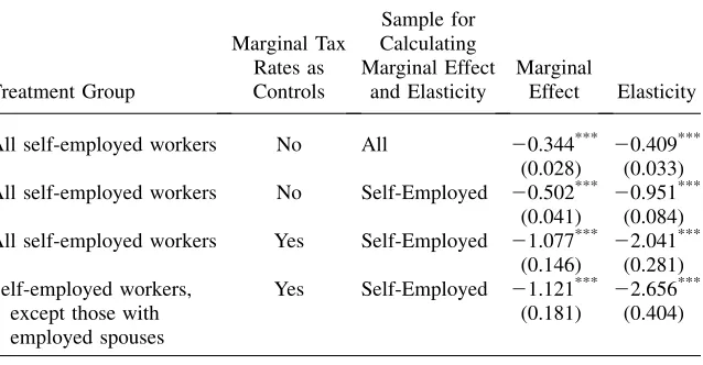
IV. Results
Table 2 presentsRP results for workers in an effort to replicate as nearly as possible the results from Table V in G&P and to clarify other differences in my approach. The first row follows G&P’s methodology, yielding a marginal ef-fect of -0.344.29The associated elasticity is -0.409, obtained by multiplying the mar-ginal effect times the sample average of RP and dividing by the sample average private coverage rate. In view of the differences in data source, period of analysis, and policy change being studied, these are remarkably close to G&P’s findings of a marginal effect of -0.248 and an elasticity of -0.28.30
Three methodological changes yield substantially higher results. The first is to use the same coefficient estimates, but to compute the marginal effect and elasticity using only self-employed workers in 2004, rather than the entire sample of employed and self-employed workers.31 Doing so yields a more policy-relevant effect of the treatment on the treated. This increases the marginal effect by a factor of nearly 1.5. Indeed, the elasticity more than doubles, because self-employed workers have higherRP and lower coverage rates than the overall sample. Adding marginal tax rates as control variables for confounding tax bracket effects yields a marginal effect of -1.077 and an elasticity of -2.041, with little loss of precision (the relative standard errors increase only slightly). In the final row of Table 2, I treat workers in mixed employed/self-employed families as if they were employed. On average across years, 42.2 percent of all self-employed workers are in mixed families (s.e.¼0.8). Legally, self-employed workers are only eligible for the self-employed premium deduction if they do not have an employed spouse who is offered coverage. More fundamentally, mixed families look more like the employed than the self-employed on all relevant dimensions, including insurance coverage, and the main pathway to insurance cov-erage for these families is through ESI held by the employed spouse.32 Refining the treatment group in this way yields an incrementally larger marginal effect of -1.121. The elasticity increases more, to -2.656, because private coverage rates in purely self-employed families are lower than in mixed families.
This elasticity might strike some readers as being implausible large. However, sev-eral comments are in order. First, whereas estimates at the top of Table 2 are close to G&P’s RP results, their unadjusted difference-in-differences estimate of 0.067 (G&P, Table VI) translates into a self-employed marginal effect of -0.91 (dividing by the RP
29. Following G&P, I calculate marginal effects by adding a small (0.01) increase inRPto each observa-tion and computing the mean change in the predicted probabilities.
30. G&P report the semi-elasticity, which I have converted to an elasticity using coverage estimates for self-employed and employed workers from their Table IV.
31. The 2004 sample is used because the self-employed population changed over time and results for the most recent group of employed are most relevant for policy. Results for the entire group of self-employed, however, are very similar.
32. For example, the private coverage rate in 2004 among adults in mixed employment families was 82.9 percent (s.e.¼2.0) versus 77.9 percent (s.e. 0.6) among all adults in employed families and 47.9 percent (s.e.¼2.6) among adults in purely self-employed families.
difference-in-differences) and an elasticity of -1.74 (multiplying and dividing by av-erage RP and avav-erage covav-erage, respectively). Furthermore, G&P’s preferred and most frequently cited result is the unmarried worker semi-elasticity from their mul-tivariate differences-in-differences model. That estimate, like the estimates at the bottom of Table 2, avoids both the problem of omitted marginal tax rates and the confounding effects of mixed employment among self-employed workers with employed spouses. Their semi-elasticity estimate of -1.78 is substantially larger than the semi-elasticity of -1.238 corresponding to the bottom row of Table 2.33
A second consideration is that RP-based estimates are intrinsically different from results based onTP, which are more commonly reported in the tax price literature. TheTPmodel corresponding to the RP results in the last row of Table 2 yields a mar-ginal effect of -1.023 (s.e.¼0.192) and an elasticity of -1.783 (s.e.¼0.326).34
Third, it is important to distinguish betweentax price elasticities and premium
elasticities. Premium elasticities reflect the impact on coverage of a one dollar
Table 2
Impact of Methodology on Results for Private Coverage of Self-Employed Workers
Treatment Group
Marginal Tax Rates as Controls
Sample for Calculating Marginal Effect
and Elasticity
Marginal
Effect Elasticity
All self-employed workers No All 20.344*** 20.409***
(0.028) (0.033)
All self-employed workers No Self-Employed 20.502*** 20.951***
(0.041) (0.084)
All self-employed workers Yes Self-Employed 21.077*** 22.041***
(0.146) (0.281)
Self-employed workers, except those with employed spouses
Yes Self-Employed 21.121*** 22.656***
(0.181) (0.404)
Results based on G&P’s relative price measure (RP), which measures the cost of acquiring health care if privately insured (inclusive of loading factors and all tax subsidies) divided by the cost of acquiring health care if uninsured (adjusting only for the potential itemization of excess medical spending). Marginal effects are changes in coverage probabilities in response to a 0.01 increase in the price. Elasticities computed by multiplying the marginal effect by mean price and dividing by mean coverage rate. Standard errors (in pa-rentheses) are adjusted for the complex design of the survey using the method of balanced repeated repli-cates.***Denotes significantly different from zero at 1 percent level.
33. Semi-elasticity is the marginal effect times the average price. Dividing G&P’s semi-elasticity by their 52 percent average private coverage rate for unmarried self-employed workers yields an elasticity of -3.42. Note, however, that it is difficult to interpret G&P’s multivariate DD results insofar as marginal effects were calculated based on changing only the interaction term in their probit equation (Ai and Norton 2003). 34. Adjusting theRPresults using the average derivative ofRPwith respect toTPin the sample yields results very similar to those reported forTP, showing that theRPandTPresults are essentially measuring the same responses.
increase in the premium and have generally been found to be smaller than -0.5 even in the small group and nongroup markets.35However, premium-based results fre-quently reflect changes in underlying medical costs, health risks, and benefits – all of which are likely to affect demand for coverage.36
Fourth, it is reasonable to expect larger marginal effects and elasticities for the self-employed than for the employed groups studied in most other tax price analyses. The entrepreneurial nature of the self-employed, combined with the small sizes of most self-employed enterprises and the higher loading factors they face, may trans-late into greater responsiveness to price signals. In fact, computing marginal effects and elasticities foremployedworkers based on the model at the bottom of Table 2 yields a marginal effect of -0.762 (s.e.¼0.125) and an elasticity of -0.883 (s.e.¼0.147). Corresponding TP-based estimates for employed workers are a mar-ginal effect of -0.699 (s.e.¼0.137) and an elasticity of -0.604 (s.e.¼0.119). These are approximately at the midpoint of the tax price literature foremployedworkers, thereby providing an important validity check on theself-employedresults.37
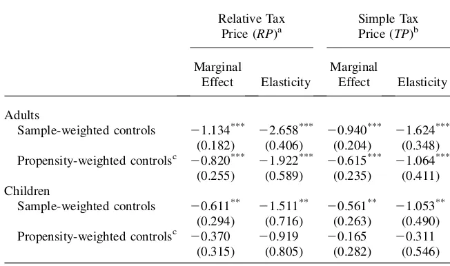
Table 3 expands the analysis to include all adults and children in self-employed (and employed) families. The main (sample weighted) results for adults mirror those for workers. In contrast, applying propensity score adjusted weights to the control group yields smaller marginal effects and elasticities. These estimates, however, have larger relative standard errors than the sample-weighted results, reflecting at least in part the smaller effective sample size in the propensity-weighted models.
The bottom portion of Table 3 presents results for children. Marginal effect point estimates are smaller for children than for adults, although the differences are not statistically significant. Smaller marginal effects for children’s coverage are consis-tent with parents being more risk averse regarding children’s coverage than adults in
35. A partial list of premium-based studies includes Chernew, Frick, and McLaughlin (1997); Short and Taylor (1989); Marquis and Long (1995, 2001); Feldman et al. (1997); Blumberg, Nichols, and Banthin (2001); Cooper and Vistnes (2003); Cutler (2003); Marquis et al. (2004); Monheit and Vistnes (2005); Buchmueller and Ohri (2006); Auerbach and Ohri (2006).
36. One study that does isolate the pure effect of premium changes finds an elasticity of only -0.16 (Buchmueller and Ohri 2006). However, this result is for early retirees aged 55-64, and the applicability to the self-employed is unclear.
37. Royalty’s (2000) analysis of offers among employed workers between 1988 and 1993 finds a marginal effect of -0.90 with respect to the combined marginal tax rate (rather thanTPorRP). Adjusting her esti-mates using the mean derivative ofTPwith respect to the combined marginal tax rate in my sample yields a
TP-comparable marginal effect of -0.97. Gruber (2002) uses data on workers from 1988-1999 to find aTP
offer effect of -0.94 and aTPeffect on having private coverage from one’s own employer of -0.69. A similar analysis by Gruber and McKnight (2003) for 1982-1996, with a somewhat different set of control variables, yields a marginal effect for coverage from one’s own employer of -0.543. Bernard and Selden (2003) use data from 1987 and 1996 to findTP-based offer and private coverage marginal effects of -0.728 and -0.804 for employed workers. Chernew, Cutler, and Keenan (2005a) find a marginal effect for all adults of -0.52 (versus a wrong-signed effect in Chernew, Cutler, and Keenan 2005b). Gruber and Lettau (2004) use firm-level data to examine the effect ofTPon offers to full-time workers, finding a marginal effect of -0.357. Their elasticity for employer premium contributions is -0.71. Thomasson (2003) finds an elasticity for employer offers of -0.54 from the 1954 codification of the employer exclusion (al-though many firms were already excluding premium based on court rulings). As a final check, I reestimate the model using only employed workers in single-location firms with fewer than 50 work-ers. The (RP) marginal effect for employed workers increases to -0.893 (s.e.¼0.215), with an elas-ticity of -1.406 (s.e.¼0.338), mirroring the findings in Bernard and Selden (2003) and Gruber and Lettau (2004) that marginal effects and elasticities are larger in smaller firms.
general are about their own. Widespread children’s eligibility for public coverage also may have weakened the relationship between the tax subsidy and coverage.
The models in Table 3 were reestimated under a variety of different specifications to gain additional insights. First, I refined the sample by excluding families that lacked a full-time worker, had a member who switched between self-employed and employed status during the year, or had a member with any of the following cov-erage types: covcov-erage from a policyholder in a different household (as can happen after a divorce), retirement coverage (including Medicare for family members age 65 and over), TRICARE coverage, or COBRA coverage.38Part-time workers were far less likely than full-time workers to have been eligible for employment-related coverage, so that the employed group values ofTPandRPmay in essence introduce measurement error for these cases. Assigning appropriate prices is also complicated
Table 3
Private Coverage Results for All Family Members
Relative Tax Price (RP)a
Simple Tax Price (TP)b
Marginal
Effect Elasticity
Marginal
Effect Elasticity
Adults
Sample-weighted controls 21.134*** 22.658*** 20.940*** 21.624***
(0.182) (0.406) (0.204) (0.348)
Propensity-weighted controlsc 20.820*** 21.922*** 20.615*** 21.064***
(0.255) (0.589) (0.235) (0.411)
Children
Sample-weighted controls 20.611**
21.511** 20.561** 21.053**
(0.294) (0.716) (0.263) (0.490)
Propensity-weighted controlsc 20.370 20.919 20.165 20.311
(0.315) (0.805) (0.282) (0.546)
Marginal effects are changes in coverage probabilities in response to a 0.01 change in the price. Elasticities computed by multiplying the marginal effect by mean price and dividing by mean coverage rate. Standard errors (in parentheses) are adjusted for the complex design of the survey using the method of balanced re-peated replicates.***Denotes significantly different from zero at 1 percent level.**Denotes significantly
dif-ferent from zero at 5 percent level.
a. Relative price measures the cost of acquiring health care if privately insured (inclusive of loading factors and all tax subsidies) divided by the cost of acquiring health care if uninsured (adjusting only for the po-tential itemization of excess medical spending).
b. Simple tax price equals (1 -tFED-tST-tSS)/(1 +tSS) if employed or 1 -uFEDtFED-uSTtSTif self-employed, wheretFED,tST, andtSSare the marginal tax rates for federal income, state income, and Social Security/ Medicare, and whereuFEDanduSTare the percentages of self-employed premiums excludable from federal and state income taxes.
38. TRICARE is coverage for families of active duty and retired military personnel. COBRA coverage is for workers recently losing employment-related coverage due to a job change.
by changes in employment status during the year. With respect to the excluded forms of coverage, families with these coverage types may have faced coverage decisions that were less strongly driven by the tax subsidies associated with current employ-ment. These forms of coverage were more prevalent than one might expect. Pooling across years, the percentages of adults in employed and self-employed families with coverage of these types are 8.3 percent (s.e.¼0.2) and 12.7 percent (s.e.¼0.7), respectively. The hypothesis is that responsiveness to incentives should be larger in the narrower sample, and the marginal effects and elasticities are indeed slightly larger (but not significantly). For example, the sample-weighted RP model for adults yields a marginal effect of -1.144 (s.e.¼0.258) and an elasticity of -2.842 (s.e.¼0.666).
Next, I experimented with using the mixed employment families as a control group for the purely self-employed.39This modestly reduced the estimated effects
(but not significantly). For example, theRP-based model for adults yields a marginal effect of -0.810 (s.e.¼0.257) and an elasticity of -1.897 (s.e.¼0.593).
The results in Tables 2 and 3 impose the assumption that tax price responses of the employed and self-employed groups can be adequately modeled using a common tax-price coefficient in the probit equation. Interacting the self-employed indicator with the tax price in theRPmodel yields a significant coefficient on this interaction term, increasing the marginal effect to -1.641 (s.e.¼0.433) and the elasticity to -3.845 (s.e.¼0.977). In theTPmodel, the interaction term is not statistically sig-nificant, and the self-employed marginal effect decreases slightly to -0.861 (s.e.¼0.501), with an elasticity of -1.487 (s.e.¼0.867). Perhaps not surprisingly, these estimates are substantially less precise than the results in Table 3. However, they provide some reassurance that large self-employed responses are not solely arti-facts of imposing a common tax price response in the probit equations.40
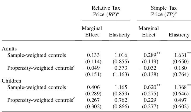
A. Results for Public Coverage
There has been substantial interest among economists and policymakers in the extent to which public coverage expansions ‘‘crowd out’’ private coverage. The reverse pro-cess can also occur, whereby increased subsidies for private coverage lead to reduced reliance on public coverage. Much of the tax price literature has ignored this possi-bility. A notable exception is Gruber (2002), who finds a (TP) public coverage mar-ginal effect of 0.162 for employed adults. Table 4 presents results from reestimating the models from Table 3 using public coverage as the dependent variable.41Point estimates of adult responses are much smaller for public coverage than for private coverage, and the sample-weighted results are approximately in line with Gruber’s finding. Point estimates also are much larger for children than for adults, as seems reasonable given that eligibility expansions were targeted more heavily at children.
39. To some extent this is in the spirit of Holtz-Eakin, Penrod, and Rosen (1996), who argue that workers with employed spouses holding ESI coverage can serve as a control group for workers lacking spousal cov-erage in their analysis of transitions to self-employment.
40. Unlike estimates relying on a common price coefficient, the models estimated with separate price responses are fairly unstable across minor specification changes. I also tried estimating a completely sep-arate model using just the self-employed sample, but this proved highly unstable and imprecise. 41. See also Gruber (2002).
However, the public coverage results are rarely significant and vary across model. In particular, the propensity-weighted models yield adult responses very close to zero. Thus, these results should not be viewed as strong evidence of reverse crowd out.
V. Simulation
Additional insight into the results in Tables 3 and 4 can be gained by simulating the budgetary and coverage effects of the post-1996 federal and state sub-sidy increases. The simulation population includes all self-employed persons in 2004 who were eligible for the health insurance subsidy and their family members.42The
Table 4
Public Coverage Results for All Family Members
Relative Tax Price (RP)a
Simple Tax Price (TP)b
Marginal
Effect Elasticity
Marginal
Effect Elasticity
Adults
Sample-weighted controls 0.133 1.016 0.289** 1.631**
(0.114) (0.855) (0.119) (0.650)
Propensity-weighted controlsc 20.049 20.373 20.032 20.180
(0.151) (1.163) (0.138) (0.764)
Children
Sample-weighted controls 0.406 1.165 0.620** 1.368**
(0.289) (0.859) (0.275) (0.646)
Propensity-weighted controlsc 0.267 0.762 0.229 0.497
(0.302) (0.866) (0.277) (0.602)
Marginal effects are changes in coverage probabilities in response to a 0.01 change in the price. Elasticities computed by multiplying the marginal effect by mean price and dividing by mean coverage rate. Standard errors (in parentheses) are adjusted for the complex design of the survey using the method of balanced re-peated replicates.***Denotes significantly different from zero at 1 percent level.**Denotes significantly
dif-ferent from zero at 5 percent level.
a. Relative price measures the cost of acquiring health care if privately insured (inclusive of loading factors and all tax subsidies) divided by the cost of acquiring health care if uninsured (adjusting only for the po-tential itemization of excess medical spending).
b. Simple tax price equals (1 -tFED-tST-tSS)/(1 +tSS) if employed or 1 -uFEDtFED-uSTtSTif self-employed, wheretFED,tST, andtSSare the marginal tax rates for federal income, state income, and Social Security/Medicare, and whereuFEDanduSTare the percentages of self-employed premiums excludable from federal and state income taxes.
42. This includes a small group of two-earner families with mixed employment in which the employed spouse was not eligible for ESI. I reedited MEPS insurance premiums for the entire subsidy-eligible group to ensure that self-employed or policyholders with missing premiums received imputed amounts from donors who were also self-employed (amounts on the public use file appear not to have been edited with this specific application in mind).
2004 status quo can be constructed simply by applying tax subsidy rules to premiums paid by eligible persons. The counterfactual is that federal and state deductibility had remained at 1996 levels (a change inu from Equation 1). Applying the estimated
models to the sample of subsidy-eligible persons with private coverage, I compute the probability, conditional on having coverage in 2004, that the person would have been privately insured given 1996 subsidies.43I then consider two alternative
scenar-ios. In case A, I ignore the possibility of reverse crowd out, assuming that all persons gaining private coverage due to the post-1996 subsidy increases would otherwise have been uninsured. In case B, I use the estimated public coverage models in Table 4, despite concerns about their reliability, thereby allowing for varying degrees of re-verse crowd out.
Table 5 presents the simulation results. The top panel provides basic details re-garding the baseline or status quo simulation. The total tax subsidy was $4.23 billion (2004 dollars).44Averaged over the 11.8 million subsidy-eligible persons observed to have private coverage, the average subsidy was $359.
The bottom panel of Table 5 shows the simulated impact of the post-1996 federal and state subsidy increases. Starting with case A, the total number of persons simu-lated to have gained private coverage from the post-1996 subsidy increases ranges from 1.1 million to 1.7 million, with simulations based on the propensity-weighted results yielding the smallest coverage increases. The cost of increasing the subsidy varies far less, ranging from $2.37 billion to $2.43 billion. Mirroring the pattern of simulated coverage changes, the cost per person who would otherwise have been uninsured ranges from $1,435 to $2,171. Because 80 to 90 percent of the simulation population would have had coverage in the absence of a subsidy increase, much of this cost can be viewed as an inframarginal transfer that ranged from a low of $186 dollars per person in the sample-weightedRP model to a high of $193 in the propensity-weightedTPmodel (not shown in table).
Case B allows subsidy changes to have affected public coverage. The private cov-erage increase is the same as in case A, but now reverse crowd out reduces public coverage by 0.1 million in the propensity-weighted models to 0.6 million in the sample-weightedTPmodel. The reduction in tax revenue is nearly the same as in case A.45However, the subsidy per insured person in 2004 is far below the average cost of public insurance ($1,818),46so that savings from reduced public insurance spending partially offset the revenue reduction. As a result, the total cost of the post-1996 subsidy increase ranges from $1.34 billion to $2.25 billion. For the sample-weighted models, reverse crowd out also reduces the cost per newly insured person to
43. Let A and B represent having private coverage atu96 andu04, respectively. From basic probability theory, P(A)¼P(AjB)P(B) + P(AjB#)P(B#). Assuming that higher subsidies cause no one to drop coverage, we have P(AjB#)¼0, so that P(AjB)¼P(A)/P(B). Because these conditional probabilities do not exactly match the overall marginal effect from the 1996 to 2004 subsidy change, I adjust them downward by scaling factors ranging from 0.990 to 0.996 (depending on the model).
44. The federal-only subsidy for premiums, at $3.30 billion, is virtually the same as the corresponding De-partment of Treasury estimate of $3.33 billion for fiscal year 2004 (Office of Management and Budget 2006).
45. Allowing for reverse crowd-out slightly increases the revenue reduction, because uninsured persons have higher expected medical expense deductions.
46. This is weighted by the mix of children and adults simulated to be leaving public coverage.
Table 5
Simulated Impact of Post-1996 Changes in Federal and State Tax Subsidies, Self-Employed Families in 2004
Benchmark simulation (subsidy In 2004)
Total (millions) Share (percent)
Persons in eligible self-employed families 22.4 (1.2) 100.0
Privately insured 11.8 (0.9) 52.6 (2.3)
Publicly insured 6.0 (0.5) 26.6 (1.8)
Uninsured 6.4 (0.5) 28.5 (1.7)
Federal Revenue Loss
State
Revenue Loss Total
Benchmark tax subsidy in 2004
Premium subsidy ($ billions) 3.30 (0.29) 0.72 (0.08) 4.02 (0.35)
Excess medical expense subsidy ($ billions) 0.17 (0.05) 0.04 (0.01) 0.21 (0.06)
Total ($ billions) 3.47 (0.32) 0.76 (0.08) 4.23 (0.35)
Tax subsidy per insured person ($) 359 (26)
134
The
Journal
of
Human
Impact of Subsidy Increase
Main Results
(RP)
Main Results
(TP)
Propensity-Weighted
(RP)
Propensity-Weighted
(TP)
Case A: No change in public coverage Coverage changes from subsidy increase
Change in private (millions) 1.6 (0.1) 1.7 (0.1) 1.1 (0.1) 1.1 (0.1)
Change in public (millions) NA NA NA NA
Change in uninsured (millions) 21.6 (0.1) 21.7 (0.1) 21.1 (0.1) 21.1 (0.1)
Budgetary impact of subsidy increase
Decreased tax revenue ($ billions) 2.43 (0.22) 2.42 (0.22) 2.39 (0.21) 2.37 (0.21)
Decreased public insurance spending ($ billions) NA NA NA NA
Net cost ($ billions) 2.43 (0.22) 2.42 (0.22) 2.39 (0.21) 2.37 (0.21)
Net cost per newly insured ($) 1,547 (117) 1,435 (117) 2,096 (163) 2,171 (174)
Case B: Subsidy reduces public coverage Coverage changes from subsidy increase
Change in private (millions) 1.6 (0.1) 1.7 (0.1) 1.1 (0.1) 1.1 (0.1)
Change in public (millions) 20.3 (0.02) 20.6 (0.1) 20.1 (0.01) 20.1 (0.1)
Change in uninsured (millions) 21.3 (0.1) 21.1 (0.1) 21.1 (0.1) 21.0 (0.1)
Budgetary impact of subsidy increase
Decreased tax revenue ($ billions) 2.45 (0.22) 2.48 (0.22) 2.40 (0.21) 2.38 (0.21)
Decreased public insurance spending ($ billions) 0.52 (0.07) 1.14 (0.15) 0.15 (0.02) 0.19 (0.02)
Net cost ($ billions) 1.93 (0.21) 1.34 (0.22) 2.25 (0.18) 2.20 (0.21)
Net cost per newly insured ($) 1,485 (149) 1,245 (215) 2,117 (176) 2,210 (193)
Standard errors (in parentheses) are adjusted for the complex design of the survey, but do not capture sampling variation in the coefficient estimates used to simulate
coverage changes. Selden
$1,245 or $1,485. For the propensity-weighted models, reverse crowd out modestly increases the cost per newly insured, because the cost per newly insured in case A exceeds the cost of public coverage.
The models yield a substantial range of estimates for the cost per newly insured person, from $1,245 to $2,210. Nevertheless, even at the upper end of this range, re-ducing uninsurance via increased subsidies for self-employed health insurance was less expensive than the simulated costs per newly insured person of $3,707 to $19,501 found by Gruber (2005) in his analysis of more broadly targeted reforms.47 Intuitively, low private coverage rates in this population help to reduce inframarginal transfers to those who would have held coverage absent the subsidy increases, while the estimated tax subsidy responses yield relatively large increases in the number of persons with private coverage.
VI. Discussion
This paper presents new estimates of the subsidy responsiveness of coverage among the self-employed. The expanded tax deduction for premiums paid by self-employed workers provides a valuable ‘‘natural experiment’’ to estimate tax subsidy responses. Increased tax subsidies were associated with large increases in private coverage among the self-employed. Among adults in self-employed families, the main (sample-weighted) results indicate a marginal effect of -1.134 using G&P’s relative price, with an associated elasticity of -2.658. The propensity score weighted model yields a somewhat smaller marginal effect of -0.820, with an elasticity of -1.922. Private coverage for children in self-employed families appears to be less sensitive to subsidies, although estimates for children tend to be less precise. In ad-dition to these private coverage results, there is some evidence suggesting that tax subsidies may help ‘‘crowd out’’ public coverage, especially among children, al-though the magnitude and significance of this effect vary across specifications.
The post-1996 federal and state subsidy increases are simulated to have increased private coverage in 2004 by 1.1 to 1.7 million persons. Annual federal and state cost (in 2004 dollars) ranges from $1.9 billion to $2.4 billion, with one model yielding an estimate of $1.3 billion due to substantial estimated reductions in public coverage. As in any subsidy-based effort to expand private coverage, much of the cost arises from inframarginal transfers to families that would have held coverage even in the absence of a subsidy increase, and evaluating the merits of such transfers will depend largely on one’s subjective valuation of increasing the horizontal equity between self-employed and self-employed families. Nevertheless, despite substantial inframarginal transfers, the cost per newly insured person ranged from $1,245 to $2,210—amounts that are below the costs found in comparable simulations of more broadly targeted subsidies.
The analysis stops short of making policy recommendations with respect to nar-rowing the remaining gap between subsidies for employed and self-employed work-ers by excluding self-employed premiums from the self-employment tax. The results
47. These estimates are for reforms that would yield a net reduction in uninsurance of three million per-sons. Larger reductions in uninsurance are estimated to entail higher costs per newly insured.
suggest that removing this disparity might appeal to a broad constituency, combining proponents of entrepreneurship, advocates for children and families, and those seek-ing easily applied policy tools for helpseek-ing to strengthen the private coverage market. However, the self-employment tax differs substantially from the income taxes that provide much of the identifying variation for the results in this paper. Like payroll taxes paid by employers and employed workers, the self-employment tax is constant across a wide range of income levels (with a phase-out only at high incomes). Allow-ing the self-employed to deduct premiums from the basis for this tax would have a more progressive incidence than the reforms to date, and the effect on coverage might therefore differ in unknown ways from the results presented here.
References
Ai, Chunrong, and Edward C. Norton. 2003. ‘‘Interaction Terms in Logit and Probit Models.’’ Economic Letters80:123–29.
Anderson, Gerald F. 2007. ‘‘FromÔSoak the RichÕtoÔSoak the PoorÕ: Recent Trends in Hospital Pricing.’’Health Affairs26(3):780–89.
Auerbach, David, and Sabina Ohri. 2006. ‘‘The Price Sensitivity of Demand for Nongroup Health Insurance.’’Inquiry43(2):122–34.
Bernard, Didem, and Thomas M. Selden. 2003. ‘‘Employer Offers, Private Coverage, and the Tax Subsidy for Health Insurance: 1987 and 1996.’’International Journal of Health Care Finance and Economics2(4):297–318.
__________. 2006. ‘‘Workers Who Decline Employment-Related Health Insurance.’’ Medical Care44(5 Supplement):I-12–I-18.
Blumberg, Linda, Len Nichols, and Jessica Banthin. 2001. ‘‘Worker Decisions to Purchase Health Insurance.’’International Journal of Health Care Finance and Economics1(3/4): 305–25.
Buchmueller, Thomas C., and Sabina Ohri. 2006. ‘‘Health Insurance Take-up by the Near Elderly.’’Health Services Research41(6):2054–73.
Bundorf, M. Kate, Bradley Herring, and Mark V. Pauly. 2005. ‘‘Health Risk, Income, and the Purchase of Private Health Insurance.’’ NBER Working Paper, No. 11677. Cambridge, Mass.: National Bureau of Economic Research.
Bureau of Labor Statistics. 2004.Historical Data for the ‘‘A’’ Tables of the Employment Situation News Release, Table A-5, downloaded July 19, 2006 from http://www.bls.gov/ cps/cpsatabs.htm.
Burman, Leonard E., Cori E. Uccello, Laura L. Wheaton, Deborah Kobes. 2003. ‘‘Tax Incentives for Health Insurance.’’ Urban Institute and Brookings Institution Tax Policy Center, Discussion Paper No. 12, downloaded September 24, 2007 from http://www. taxpolicycenter.org/publications/url.cfm?ID¼310791.
Chernew, Michael, David M. Cutler, and Patricia S. Keenan. 2005a. ‘‘Charity Care, Risk Pooling, and the Decline in Private Health Insurance.’’American Economic Review, Papers and Proceedings95(2):209–13.
__________. 2005b. ‘‘Increasing Health Insurance Costs and the Decline in Insurance Coverage.’’Health Services Research40(4):1021–39.
Chernew, Michael, Kevin Frick, and Catherine G. McLaughlin. 1997. ‘‘The Demand for Health Insurance Coverage by Low-Income Workers: Can Reduced Premiums Achieve Full Coverage?’’Health Services Research32(4):453–70.
Cohen, Joel W., Alan C. Monheit, Karen M. Beauregard, et al. 1996. ‘‘The Medical
Expenditure Panel Survey: A National Health Information Resource.’’Inquiry33(4):373–89.
Cohen, Steven B. 1997.Sample Design of the 1996 Medical Expenditure Panel Survey Household Component.MEPS Methodology Report No. 2, Pub. No. 97-0027. Rockville, Md.: Agency for Health Care Policy and Research.
Cooper, Philip F., and Jessica Vistnes. 2003. ‘‘Workers’ Decisions to Take-Up Offered Health Insurance Coverage: Assessing the Importance of Out-of-Pocket Premium Costs.’’Medical Care41(7 Supplement):III-35 - III-43.
Cutler, David M. 2003. ‘‘Employee Costs and the Decline in Health Insurance Coverage,’’ Frontiers in Health Policy Research6. Downloaded August 25, 2006 from http://www. bepress.com/fhep/6/.
Feenberg, Daniel. 1989. ‘‘Are Tax Price Models Really Identified: The Case of Charitable Giving.’’National Tax Journal40(4):629–33.
Feenberg, Daniel and Elisabeth Coutts. 1993. ‘‘An Introduction to the TAXSIM Model.’’ Journal of Policy Analysis and Management12(1):189–94.
Feldman, Roger, Brian Dowd, Scott Leitz, and Lynn A. Blewett. 1997. ‘‘The Effect of Premiums on the Small Firms Decision to Offer Health Insurance.’’Journal of Human Resources32(4):635–58.
Gruber, Jonathan. 2002. ‘‘The Impact of the Tax System on Health Insurance Coverage.’’ International Journal of Health Care Finance and Economics1(3/4):293–304.
Gruber, Jonathan. 2005. ‘‘Tax Policy for Health Insurance.’’ InTax Policy and the Economy 19.Ed. James Poterba, 39-63, Cambridge, Mass.: MIT Press.
Gruber, Jonathan, and Michael Lettau. 2004. ‘‘How Elastic is the Firm’s Demand for Health Insurance?’’Journal of Public Economics88(7):1273–94.
Gruber, Jonathan, and Robin McKnight. 2003. ‘‘Why Did Employee Health Insurance Contributions Rise?’’Journal of Health Economics22(6):1085–1104.
Gruber, Jonathan, and James Poterba. 1994. ‘‘Tax Incentives and the Decision to Purchase Health Insurance: Evidence from the Self-Employed.’’Quarterly Journal of Economics 109(3):701–34.
___________. 1996a. ‘‘Tax Subsidies to Employer-Provided Health Insurance.’’ InEmpirical Foundations of Household Taxation.Ed. Martin Feldstein and James M. Poterba, 135-64, Chicago: The University of Chicago Press.
__________. 1996b. ‘‘Fundamental Tax Reform and Employer-Provided Health Insurance.’’ InEconomic Effects of Fundamental Tax Reform, ed. Henry J. Aaron and William G. Gale, 125-62. Washington, D.C.: The Brookings Institution Press.
Holtz-Eakin, Douglas, John R. Penrod, and Harvey S. Rosen. 1996. ‘‘Health Insurance and the Supply of Entrepreneurs.’’Journal of Public Economics62(1/2):209–35.
Internal Revenue Service. 2001 and 2002.Earned Income Tax Credit.Publication 596, downloaded May 10, 2007 from http://www.irs.gov/formspubs/index.html.
Marquis, M. Susan, and Stephen H. Long. 1995. ‘‘Worker Demand for Health Insurance in the Nongroup Market.’’Journal of Health Economics14(1):47–63.
Marquis, M. Susan, and Stephen H. Long. 2001. ‘‘To Offer or Not to Offer: The Role of Price in Employers’ Health Insurance Decisions.’’Health Services Research36(5):935–58. Marquis, M. Susan, Melinda Beeuwkes Buntin, Jose´ J. Escarce, Kanika Kapur, and Jill M.
Yegian. 2004. ‘‘Subsidies and the Demand for Individual Health Insurance in California.’’ Health Services Research39(5):1547–70.
Meer, Jonathan, and Harvey S. Rosen. 2004. ‘‘Insurance and the Utilization of Medical Services.’’Social Science and Medicine58(9):1623–32.
Monheit, Alan C., and P. Holly Harvey. 1993. ‘‘Sources of Health Insurance for the Self-Employed: Does Differential Taxation Make a Difference?’’Inquiry30(3):293–305. Monheit, Alan C., and Jessica P. Vistnes. 1997.Health Insurance Status of Workers and Their
Families: 1996.MEPS Research Findings No. 2, Pub. No. 97-0065. Rockville, Md.: Agency for Health Care Policy and Research.