This textbook is an expanded version of Elementary Linear Algebra, Ninth Edition, by Howard Anton. The first ten chapters of this book are identical to the first ten chapters of that text; the eleventh chapter consists of 21 applications of linear algebra drawn from business, economics, engineering, physics, computer science, approximation theory, ecology, sociology,
demography, and genetics. The applications are, with one exception, independent of one another and each comes with a list of mathematical prerequisites. Thus, each instructor has the flexibility to choose those applications that are suitable for his or her students and to incorporate each application anywhere in the course after the mathematical prerequisites have been satisfied. This edition of Elementary Linear Algebra, like those that have preceded it, gives an elementary treatment of linear algebra that is suitable for students in their freshman or sophomore year. The aim is to present the fundamentals of linear algebra in the clearest possibleway; pedagogy is the main consideration. Calculus is not a prerequisite, but there are clearly labeled exercises and examples for students who have studied calculus. Those exercises can be omitted without loss of continuity. Technology is also not required, but for those who would like to use MATLAB, Maple, Mathematica, or calculators with linear algebra
capabilities, exercises have been included at the ends of the chapters that allow for further exploration of that chapter's contents.
This edition contains organizational changes and additional material suggested by users of the text. Most of the text is unchanged. The entire text has been reviewed for accuracy, typographical errors, and areas where the exposition could be improved or additional examples are needed. The following changes have been made:
Section 6.5 has been split into two sections: Section 6.5 Change of Basis and Section 6.6 Orthogonal Matrices. This allows for sharper focus on each topic.
A new Section 4.4 Spaces of Polynomials has been added to further smooth the transition to general linear transformations, and a new Section 8.6 Isomorphisms has been added to provide explicit coverage of this topic.
Chapter 2 has been reorganized by switching Section 2.1 with Section 2.4. The cofactor expansion approach to determinants is now covered first and the combinatorial approach is now at the end of the chapter.
Additional exercises, including Discussion and Discovery, Supplementary, and Technology exercises, have been added throughout the text.
In response to instructors' requests, the number of exercises that have answers in the back of the book has been reduced considerably.
The page design has been modified to enhance the readability of the text.
Relationships Between Concepts One of the important goals of a course in linear algebra is to establish the intricate thread of relationships between systems of linear equations, matrices, determinants, vectors, linear transformations, and eigenvalues. That thread of relationships is developed through the following crescendo of theorems that link each new idea with ideas that preceded it: 1.5.3, 1.6.4, 2.3.6, 4.3.4, 5.6.9, 6.2.7, 6.4.5, 7.1.5. These theorems bring a coherence to the linear algebra landscape and also serve as a constant source of review.
Smooth Transition to Abstraction The transition from to general vector spaces is often difficult for students. To smooth out that transition, the underlying geometry of is emphasized and key ideas are developed in before proceeding to general vector spaces.
Early Exposure to Linear Transformations and Eigenvalues To ensure that the material on linear transformations and eigenvalues does not get lost at the end of the course, some of the basic concepts relating to those topics are
developed early in the text and then reviewed and expanded on when the topic is treated in more depth later in the text. For example, characteristic equations are discussed briefly in the chapter on determinants, and linear transformations from
to are discussed immediately after is introduced, then reviewed later in the context of general linear transformations.
Each section exercise set begins with routine drill problems, progresses to problems with more substance, and concludes with theoretical problems. In most sections, the main part of the exercise set is followed by the Discussion and Discovery problems described above. Most chapters end with a set of supplementary exercises that tend to be more challenging and force the student to draw on ideas from the entire chapter rather than a specific section. The technology exercises follow the
supplementary exercises and are classified according to the section in which we suggest that they be assigned. Data for these exercises in MATLAB, Maple, and Mathematica formats can be downloaded from www.wiley.com/college/anton.
!
""
This chapter consists of 21 applications of linear algebra. With one clearly marked exception, each application is in its own independent section, so that sections can be deleted or permuted freely to fit individual needs and interests. Each topic begins with a list of linear algebra prerequisites so that a reader can tell in advance if he or she has sufficient background to read the section.
Because the topics vary considerably in difficulty, we have included a subjective rating of each topic—easy, moderate, more difficult. (See “A Guide for the Instructor” following this preface.) Our evaluation is based more on the intrinsic difficulty of the material rather than the number of prerequisites; thus, a topic requiring fewer mathematical prerequisites may be rated harder than one requiring more prerequisites.
Because our primary objective is to present applications of linear algebra, proofs are often omitted. We assume that the reader has met the linear algebra prerequisites and whenever results from other fields are needed, they are stated precisely (with motivation where possible), but usually without proof.
Since there is more material in this book than can be covered in a one-semester or one-quarter course, the instructor will have to make a selection of topics. Help in making this selection is provided in the Guide for the Instructor below.
!!
#
$
%
& #
Data for Technology Exercises is provided in MATLAB, Maple, and Mathematica formats. This data can be downloaded from www.wiley.com/college/anton.
Linear Algebra Solutions—Powered by JustAsk! invites you to be a part of the solution as it walks you step-by-step through a total of over 150 problems that correlate to chapter materials to help you master key ideas. The powerful online
problem-solving tool provides you with more than just the answers.
!!
#
$
%
#
Instructor's Solutions Manual—This new supplement provides solutions to all exercises in the text. (ISBN 0-471-44798-6) Test Bank—This includes approximately 50 free-form questions, five essay questions for each chapter, and a sample
cumulative final examination. (ISBN 0-471-44797-8)
eGrade—eGrade is an online assessment system that contains a large bank of skill-building problems, homework problems, and solutions. Instructors can automate the process of assigning, delivering, grading, and routing all kinds of homework, quizzes, and tests while providing students with immediate scoring and feedback on their work. Wiley eGrade “does the math”… and much more. For more information, visit http://www.wiley.com/college/egrade or contact your Wiley representative.
Web Resources—More information about this text and its resources can be obtained from your Wiley representative or from www.wiley.com/college/anton.
Linear algebra courses vary widely between institutions in content and philosophy, but most courses fall into two categories: those with about 35–40 lectures (excluding tests and reviews) and those with about 25–30 lectures (excluding tests and reviews). Accordingly, I have created long and short templates as possible starting points for constructing a course outline. In the long template I have assumed that all sections in the indicated chapters are covered, and in the short template I have assumed that instructors will make selections from the chapters to fit the available time. Of course, these are just guides and you may want to customize them to fit your local interests and requirements.
The organization of the text has been carefully designed to make life easier for instructors working under time constraints: A brief introduction to eigenvalues and eigenvectors occurs in Sections 2.3 and 4.3, and linear transformations from to are discussed in Chapter 4. This makes it possible for all instructors to cover these topics at a basic level when the time available for their more extensive coverage in Chapters 7 and 8 is limited. Also, note that Chapter 3 can be omitted without loss of continuity for students who are already familiar with the material.
Long Template Short Template
Long Template Short Template
Chapter 7 4 lectures 3 lectures Chapter 8 6 lectures 2 lectures Total 38 lectures 27 lectures
'
# #
#&
&
Many variations in the long template are possible. For example, one might create an alternative long template by following the time allocations in the short template and devoting the remaining 11 lectures to some of the topics in Chapters 9, 10 and 11.
#
!!
# (
#
&
Once the necessary core material is covered, the instructor can choose applications from Chapter 9 or Chapter 11. The following table classifies each of the 21 sections in Chapter 11 according to difficulty:
Easy. The average student who has met the stated prerequisites should be able to read the material with no help from the instructor.
Moderate. The average student who has met the stated prerequisites may require a little help from the instructor.
More Difficult. The average student who has met the stated prerequisites will probably need help from the instructor.
1 2 3 4 5 6 7 8 9 10 11 12 13 14 15 16 17 18 19 20 21
EASY • • •
MODERATE • • • • • • • • • • •
MORE DIFFICULT
• • • • • • •
We express our appreciation for the helpful guidance provided by the following people:
Marie Aratari, Oakland Community College Nancy Childress, Arizona State University Nancy Clarke, Acadia University
Aimee Ellington, Virginia Commonwealth University William Greenberg, Virginia Tech
Molly Gregas, Finger Lakes Community College Conrad Hewitt, St. Jerome's University
Sasho Kalajdzievski, University of Manitoba
Gregory Lewis, University of Ontario Institute of Technology Sharon O'Donnell, Chicago State University
Mazi Shirvani, University of Alberta
Roxana Smarandache, San Diego State University Edward Smerek, Hiram College
Earl Taft, Rutgers University AngelaWalters, Capitol College
Special thanks are due to two very talented mathematicians who read the manuscript in detail for technical accuracy and provided excellent advice on numerous pedagogical and mathematical matters.
Philip Riley, James Madison University Laura Taalman, James Madison University
!
Jeffery J. Leader–for his outstanding work overseeing the implementation of numerous recommendations and improvements in this edition.
Chris Black, Ralph P. Grimaldi, and Marie Vanisko–for evaluating the exercise sets and making helpful recommendations. Laurie Rosatone–for the consistent and enthusiastic support and direction she has provided this project.
Jennifer Battista–for the innumerable things she has done to make this edition a reality.
Anne Scanlan-Rohrer–for her essential role in overseeing day-to-day details of the editing stage of this project. Kelly Boyle and Stacy French–for their assistance in obtaining pre-revision reviews.
Ken Santor–for his attention to detail and his superb job in managing this project.
Techsetters, Inc.–for once again providing beautiful typesetting and careful attention to detail. Dawn Stanley–for a beautiful design and cover.
The Wiley Production Staff–with special thanks to Lucille Buonocore, Maddy Lesure, Sigmund Malinowski, and Ann Berlin for their efforts behind the scenes and for their support on many books over the years.
HOWARD ANTON CHRIS RORRES
1
Systems of Linear Equations and Matrices
I
N T R O D U C T I O N : Information in science and mathematics is often organized into rows and columns to form rectangular arrays, called “matrices” (plural of “matrix”). Matrices are often tables of numerical data that arise from physical observations, but they also occur in various mathematical contexts. For example, we shall see in this chapter that to solve a system of equations such asall of the information required for the solution is embodied in the matrix
1.1
Systems of linear algebraic equations and their solutions constitute one of the major topics studied in the course known as “linear algebra.” In this first section we shall introduce some basic terminology and discuss a method for solving such systems.Any straight line in the -plane can be represented algebraically by an equation of the form
where , , and b are real constants and and are not both zero. An equation of this form is called a linear equation in the variables x and y. More generally, we define a linear equation in the n variables , , …, to be one that can be expressed in the form
where , , …, , and b are real constants. The variables in a linear equation are sometimes called unknowns.
EXAMPLE 1 Linear Equations
The equations
are linear. Observe that a linear equation does not involve any products or roots of variables. All variables occur only to the first power and do not appear as arguments for trigonometric, logarithmic, or exponential functions. The equations
are not linear.
A solution of a linear equation is a sequence of n numbers , , …, such that the equation is satisfied when we substitute , , …, . The set of all solutions of the equation is called its solution set or sometimes the general solution of the equation.
EXAMPLE 2 Finding a Solution Set
Find the solution set of (a) , and (b) .
To find solutions of (a), we can assign an arbitrary value to x and solve for y, or choose an arbitrary value for y and solve for x. If we follow the first approach and assign x an arbitrary value t, we obtain
obtained by substituting specific values for t. For example, yields the solution , ; and yields the solution
, .
If we follow the second approach and assign y the arbitrary value t, we obtain
Although these formulas are different from those obtained above, they yield the same solution set as t varies over all possible real numbers. For example, the previous formulas gave the solution , when , whereas the formulas immediately above
yield that solution when .
To find the solution set of (b), we can assign arbitrary values to any two variables and solve for the third variable. In particular, if we assign arbitrary values s and t to and , respectively, and solve for , we obtain
A finite set of linear equations in the variables , , …, is called a system of linear equations or a linear system. A sequence of numbers , , …, is called a solution of the system if , , …, is a solution of every equation in the system. For example, the system
has the solution , , since these values satisfy both equations. However, , , is not a solution since these values satisfy only the first equation in the system.
Not all systems of linear equations have solutions. For example, if we multiply the second equation of the system
by , it becomes evident that there are no solutions since the resulting equivalent system
has contradictory equations.
A system of equations that has no solutions is said to be inconsistent; if there is at least one solution of the system, it is called consistent. To illustrate the possibilities that can occur in solving systems of linear equations, consider a general system of two linear equations in the unknowns x and y:
Figure 1.1.1
The lines and may be parallel, in which case there is no intersection and consequently no solution to the system.
The lines and may intersect at only one point, in which case the system has exactly one solution.
The lines and may coincide, in which case there are infinitely many points of intersection and consequently infinitely many solutions to the system.
Although we have considered only two equations with two unknowns here, we will show later that the same three possibilities hold for arbitrary linear systems:
Every system of linear equations has no solutions, or has exactly one solution, or has infinitely many solutions.
where , , …, are the unknowns and the subscripted a's and b's denote constants. For example, a general system of three linear equations in four unknowns can be written as
The double subscripting on the coefficients of the unknowns is a useful device that is used to specify the location of the coefficient in the system. The first subscript on the coefficient indicates the equation in which the coefficient occurs, and the second subscript indicates which unknown it multiplies. Thus, is in the first equation and multiplies unknown .
If we mentally keep track of the location of the +'s, the x's, and the ='s, a system of m linear equations in n unknowns can be abbreviated by writing only the rectangular array of numbers:
This is called the augmented matrix for the system. (The term matrix is used in mathematics to denote a rectangular array of numbers. Matrices arise in many contexts, which we will consider in more detail in later sections.) For example, the augmented matrix for the system of equations
is
Remark When constructing an augmented matrix, we must write the unknowns in the same order in each equation, and the
constants must be on the right.
The basic method for solving a system of linear equations is to replace the given system by a new system that has the same solution set but is easier to solve. This new system is generally obtained in a series of steps by applying the following three types of
operations to eliminate unknowns systematically:
1. Multiply an equation through by a nonzero constant.
2. Interchange two equations.
3. Add a multiple of one equation to another.
Since the rows (horizontal lines) of an augmented matrix correspond to the equations in the associated system, these three operations correspond to the following operations on the rows of the augmented matrix:
2. Interchange two rows.
3. Add a multiple of one row to another row.
! " #
These are called elementary row operations. The following example illustrates how these operations can be used to solve systems of linear equations. Since a systematic procedure for finding solutions will be derived in the next section, it is not necessary to worry about how the steps in this example were selected. The main effort at this time should be devoted to understanding the computations and the discussion.
EXAMPLE 3 Using Elementary Row Operations
In the left column below we solve a system of linear equations by operating on the equations in the system, and in the right column we solve the same system by operating on the rows of the augmented matrix.
Add −2 times the first equation to the second to obtain Add −2 times the first row to the second to obtain
Add −3 times the first equation to the third to obtain Add −3 times the first row to the third to obtain
Multiply the second equation by to obtain Multiply the second row by to obtain
Add −3 times the second equation to the third to obtain Add −3 times the second row to the third to obtain
Add −1 times the second equation to the first to obtain Add −1 times the second row to the first to obtain
Add times the third equation to the first and times the
third equation to the second to obtain
Add times the third row to the first and times the
third row to the second to obtain
The solution , , is now evident.
Exercise Set
1.1
Click here for Just Ask!
1.
Which of the following are linear equations in , , and ?
(a)
(b)
(c)
(d)
(e)
(f)
2.
(a)
(b)
(c)
3.
Find the solution set of each of the following linear equations.
(a)
(b)
(c)
(d)
4.
Find the augmented matrix for each of the following systems of linear equations.
(a)
(b)
(c)
(d)
5.
(a)
(b)
(c)
(d)
6.
(a) Find a linear equation in the variables x and y that has the general solution , .
(b) Show that , is also the general solution of the equation in part (a).
7.
The curve shown in the accompanying figure passes through the points , , and . Show that the coefficients a, b, and c are a solution of the system of linear equations whose augmented matrix is
Figure Ex-7
8.
Consider the system of equations
9.
Show that if the linear equations and have the same solution set, then the equations are identical.
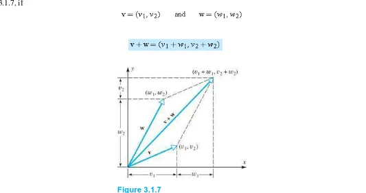
10.
Show that the elementary row operations do not affect the solution set of a linear system.
11.
For which value(s) of the constant k does the system
have no solutions? Exactly one solution? Infinitely many solutions? Explain your reasoning.
12.
Consider the system of equations
Indicate what we can say about the relative positions of the lines , , and when
(a) the system has no solutions.
(b) the system has exactly one solution.
(c) the system has infinitely many solutions.
13.
If the system of equations in Exercise 12 is consistent, explain why at least one equation can be discarded from the system without altering the solution set.
14.
If in Exercise 12, explain why the system must be consistent. What can be said about the point of intersection of the three lines if the system has exactly one solution?
15.
We could also define elementary column operations in analogy with the elementary row operations. What can you say about the effect of elementary column operations on the solution set of a linear system? How would you interpret the effects of elementary column operations?
-1.2
In this section we shall develop a systematic procedure for solving systems of linear equations. The procedure is based on the idea of reducing the augmented matrix of a system to another augmented matrix that is simple enough that the solution of the system can be found by inspection.In Example 3 of the last section, we solved a linear system in the unknowns x, y, and z by reducing the augmented matrix to the form
from which the solution , , became evident. This is an example of a matrix that is in reduced row-echelon form. To be of this form, a matrix must have the following properties:
1. If a row does not consist entirely of zeros, then the first nonzero number in the row is a 1. We call this a leading 1.
2. If there are any rows that consist entirely of zeros, then they are grouped together at the bottom of the matrix.
3. In any two successive rows that do not consist entirely of zeros, the leading 1 in the lower row occurs farther to the right than the leading 1 in the higher row.
4. Each column that contains a leading 1 has zeros everywhere else in that column.
A matrix that has the first three properties is said to be in row-echelon form. (Thus, a matrix in reduced row-echelon form is of necessity in row-echelon form, but not conversely.)
EXAMPLE 1 Row-Echelon and Reduced Row-Echelon Form
The following matrices are in reduced row-echelon form.
The following matrices are in row-echelon form.
EXAMPLE 2 More on Row-Echelon and Reduced Row-Echelon Form
As the last example illustrates, a matrix in row-echelon form has zeros below each leading 1, whereas a matrix in reduced
row-echelon form has zeros below and above each leading 1. Thus, with any real numbers substituted for the *'s, all matrices of the following types are in row-echelon form:
Moreover, all matrices of the following types are in reduced row-echelon form:
If, by a sequence of elementary row operations, the augmented matrix for a system of linear equations is put in reduced row-echelon form, then the solution set of the system will be evident by inspection or after a few simple steps. The next example illustrates this situation.
EXAMPLE 3 Solutions of Four Linear Systems
Suppose that the augmented matrix for a system of linear equations has been reduced by row operations to the given reduced row-echelon form. Solve the system.
(a)
(c)
(d)
The corresponding system of equations is
By inspection, , , .
The corresponding system of equations is
Since , , and correspond to leading 1's in the augmented matrix, we call them leading variables or pivots. The nonleading variables (in this case ) are called free variables. Solving for the leading variables in terms of the free variable gives
From this form of the equations we see that the free variable can be assigned an arbitrary value, say t, which then determines the values of the leading variables , , and . Thus there are infinitely many solutions, and the general solution is given by the formulas
The row of zeros leads to the equation , which places no restrictions on the solutions (why?). Thus, we can omit this equation and write the corresponding system as
Here the leading variables are , , and , and the free variables are and . Solving for the leading variables in terms of the free variables gives
The last equation in the corresponding system of equations is
Since this equation cannot be satisfied, there is no solution to the system.
We have just seen how easy it is to solve a system of linear equations once its augmented matrix is in reduced row-echelon form. Now we shall give a step-by-step elimination procedure that can be used to reduce any matrix to reduced row-echelon form. As we state each step in the procedure, we shall illustrate the idea by reducing the following matrix to reduced row-echelon form.
Step 1. Locate the leftmost column that does not consist entirely of zeros.
Step 2. Interchange the top row with another row, if necessary, to bring a nonzero entry to the top of the column found in Step 1.
Step 3. If the entry that is now at the top of the column found in Step 1 is a, multiply the first row by 1/a in order to introduce a leading 1.
Step 4. Add suitable multiples of the top row to the rows below so that all entries below the leading 1 become zeros.
The entire matrix is now in row-echelon form. To find the reduced row-echelon form we need the following additional step.
Step 6. Beginning with the last nonzero row and working upward, add suitable multiples of each row to the rows above to introduce zeros above the leading 1's.
The last matrix is in reduced row-echelon form.
If we use only the first five steps, the above procedure produces a row-echelon form and is called Gaussian elimination. Carrying the procedure through to the sixth step and producing a matrix in reduced row-echelon form is called Gauss–Jordan elimination.
Remark It can be shown that every matrix has a unique reduced row-echelon form; that is, one will arrive at the same reduced
Karl Friedrich Gauss
Karl Friedrich Gauss (1777–1855) was a German mathematician and scientist. Sometimes called the “prince of
mathematicians,” Gauss ranks with Isaac Newton and Archimedes as one of the three greatest mathematicians who ever lived. In the entire history of mathematics there may never have been a child so precocious as Gauss—by his own account he worked out the rudiments of arithmetic before he could talk. One day, before he was even three years old, his genius became apparent to his parents in a very dramatic way. His father was preparing the weekly payroll for the laborers under his charge while the boy watched quietly from a corner. At the end of the long and tedious calculation, Gauss informed his father that there was an error in the result and stated the answer, which he had worked out in his head. To the astonishment of his parents, a check of the computations showed Gauss to be correct!
In his doctoral dissertation Gauss gave the first complete proof of the fundamental theorem of algebra, which states that every polynomial equation has as many solutions as its degree. At age 19 he solved a problem that baffled Euclid, inscribing a regular polygon of seventeen sides in a circle using straightedge and compass; and in 1801, at age 24, he published his first masterpiece, Disquisitiones Arithmeticae, considered by many to be one of the most brilliant achievements in mathematics. In that paper Gauss systematized the study of number theory (properties of the integers) and formulated the basic concepts that form the foundation of the subject. Among his myriad achievements, Gauss discovered the Gaussian or “bell-shaped” curve that is fundamental in probability, gave the first geometric interpretation of complex numbers and established their fundamental role in mathematics, developed methods of characterizing surfaces intrinsically by means of the curves that they contain, developed the theory of conformal (angle-preserving) maps, and discovered non-Euclidean geometry 30 years before the ideas were published by others. In physics he made major contributions to the theory of lenses and capillary action, and with Wilhelm Weber he did fundamental work in electromagnetism. Gauss invented the heliotrope, bifilar magnetometer, and an electrotelegraph.
Wilhelm Jordan
Wilhelm Jordan (1842–1899) was a German engineer who specialized in geodesy. His contribution to solving linear systems appeared in his popular book, Handbuch der Vermessungskunde (Handbook of Geodesy), in 1888.
EXAMPLE 4 Gauss–Jordan Elimination
Solve by Gauss–Jordan elimination.
The augmented matrix for the system is
Adding −2 times the first row to the second and fourth rows gives
Interchanging the third and fourth rows and then multiplying the third row of the resulting matrix by gives the row-echelon form
Adding −3 times the third row to the second row and then adding 2 times the second row of the resulting matrix to the first row yields the reduced row-echelon form
The corresponding system of equations is
(We have discarded the last equation, , since it will be satisfied automatically by the solutions of the remaining equations.) Solving for the leading variables, we obtain
If we assign the free variables , , and arbitrary values r, s, and t, respectively, the general solution is given by the formulas
It is sometimes preferable to solve a system of linear equations by using Gaussian elimination to bring the augmented matrix into row-echelon form without continuing all the way to the reduced row-echelon form. When this is done, the corresponding system of equations can be solved by a technique called back-substitution. The next example illustrates the idea.
EXAMPLE 5 Example 4 Solved by Back-Substitution
From the computations in Example 4, a row-echelon form of the augmented matrix is
To solve the corresponding system of equations
we proceed as follows:
Step 2. Beginning with the bottom equation and working upward, successively substitute each equation into all the equations above it.
Substituting into the second equation yields
Substituting into the first equation yields
Step 3. Assign arbitrary values to the free variables, if any.
If we assign , , and the arbitrary values r, s, and t, respectively, the general solution is given by the formulas
This agrees with the solution obtained in Example 4.
Remark The arbitrary values that are assigned to the free variables are often called parameters. Although we shall generally use
the letters r, s, t, … for the parameters, any letters that do not conflict with the variable names may be used.
EXAMPLE 6 Gaussian Elimination
Solve
by Gaussian elimination and back-substitution.
This is the system in Example 3 of Section 1.1. In that example we converted the augmented matrix
The system corresponding to this matrix is
Solving for the leading variables yields
Substituting the bottom equation into those above yields
and substituting the second equation into the top yields , , . This agrees with the result found by Gauss–Jordan elimination in Example 3 of Section 1.1.
! "
A system of linear equations is said to be homogeneous if the constant terms are all zero; that is, the system has the form
Every homogeneous system of linear equations is consistent, since all such systems have , , …, as a solution. This solution is called the trivial solution; if there are other solutions, they are called nontrivial solutions.
Because a homogeneous linear system always has the trivial solution, there are only two possibilities for its solutions:
The system has only the trivial solution.
The system has infinitely many solutions in addition to the trivial solution.
In the special case of a homogeneous linear system of two equations in two unknowns, say
Figure 1.2.1
There is one case in which a homogeneous system is assured of having nontrivial solutions—namely, whenever the system involves more unknowns than equations. To see why, consider the following example of four equations in five unknowns.
EXAMPLE 7 Gauss–Jordan Elimination
Solve the following homogeneous system of linear equations by using Gauss–Jordan elimination.
(1)
The augmented matrix for the system is
Reducing this matrix to reduced row-echelon form, we obtain
(2)
Solving for the leading variables yields
Thus, the general solution is
Note that the trivial solution is obtained when .
Example 7 illustrates two important points about solving homogeneous systems of linear equations. First, none of the three
elementary row operations alters the final column of zeros in the augmented matrix, so the system of equations corresponding to the reduced row-echelon form of the augmented matrix must also be a homogeneous system [see system 2]. Second, depending on whether the reduced row-echelon form of the augmented matrix has any zero rows, the number of equations in the reduced system is the same as or less than the number of equations in the original system [compare systems 1 and 2]. Thus, if the given
homogeneous system has m equations in n unknowns with , and if there are r nonzero rows in the reduced row-echelon form of the augmented matrix, we will have . It follows that the system of equations corresponding to the reduced row-echelon form of the augmented matrix will have the form
(3)
where , , …, are the leading variables and denotes sums (possibly all different) that involve the free variables [compare system 3 with system 2 above]. Solving for the leading variables gives
As in Example 7, we can assign arbitrary values to the free variables on the right-hand side and thus obtain infinitely many solutions to the system.
In summary, we have the following important theorem.
T H E O R E M 1 . 2 . 1
A homogeneous system of linear equations with more unknowns than equations has infinitely many solutions.
Remark Note that Theorem 1.2.1 applies only to homogeneous systems. A nonhomogeneous system with more unknowns than
equations need not be consistent (Exercise 28); however, if the system is consistent, it will have infinitely many solutions. This will be proved later.
# $ % "
Reducing roundoff errors
Minimizing the use of computer memory space
Solving the system with maximum speed
Some of these matters will be considered in Chapter 9. For hand computations, fractions are an annoyance that often cannot be avoided. However, in some cases it is possible to avoid them by varying the elementary row operations in the right way. Thus, once the methods of Gaussian elimination and Gauss–Jordan elimination have been mastered, the reader may wish to vary the steps in specific problems to avoid fractions (see Exercise 18).
Remark Since Gauss–Jordan elimination avoids the use of back-substitution, it would seem that this method would be the more
efficient of the two methods we have considered.
It can be argued that this statement is true for solving small systems by hand since Gauss–Jordan elimination actually involves less writing. However, for large systems of equations, it has been shown that the Gauss–Jordan elimination method requires about 50% more operations than Gaussian elimination. This is an important consideration when one is working on computers.
Exercise Set
1.2
Click here for Just Ask!
1.
Which of the following matrices are in reduced row-echelon form?
(a)
(b)
(c)
(d)
(f)
(g)
(h)
(i)
(j)
2.
Which of the following matrices are in row-echelon form?
(a)
(b)
(c)
(d)
(f)
3.
In each part determine whether the matrix is in row-echelon form, reduced row-echelon form, both, or neither.
(a)
(b)
(c)
(d)
(e)
(f)
4.
In each part suppose that the augmented matrix for a system of linear equations has been reduced by row operations to the given reduced row-echelon form. Solve the system.
(a)
(c)
(d)
5.
In each part suppose that the augmented matrix for a system of linear equations has been reduced by row operations to the given row-echelon form. Solve the system.
(a)
(b)
(c)
(d)
6.
Solve each of the following systems by Gauss–Jordan elimination.
(a)
(b)
(d)
7.
Solve each of the systems in Exercise 6 by Gaussian elimination.
8.
Solve each of the following systems by Gauss–Jordan elimination.
(a)
(b)
(c)
(d)
9.
Solve each of the systems in Exercise 8 by Gaussian elimination.
10.
Solve each of the following systems by Gauss–Jordan elimination.
(a)
(c)
11.
Solve each of the systems in Exercise 10 by Gaussian elimination.
12.
Without using pencil and paper, determine which of the following homogeneous systems have nontrivial solutions.
(a)
(b)
(c)
(d)
13.
Solve the following homogeneous systems of linear equations by any method.
(a)
(b)
(c)
14.
(a)
(b)
(c)
15.
Solve the following systems by any method.
(a)
(b)
16.
Solve the following systems, where a, b, and c are constants.
(a)
(b)
17.
18.
Reduce
to reduced row-echelon form.
19.
Find two different row-echelon forms of
20.
Solve the following system of nonlinear equations for the unknown angles α, β, and γ, where , , and .
21.
Show that the following nonlinear system has 18 solutions if , , and .
22.
For which value(s) of λ does the system of equations
have nontrivial solutions?
23.
Solve the system
for , , and in the two cases , .
24.
Solve the following system for x, y, and z.
25.
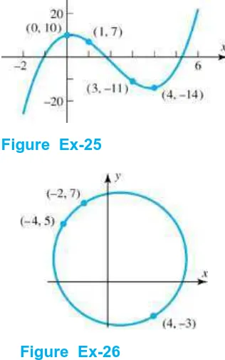
Find the coefficients a, b, c, and d so that the curve shown in the accompanying figure is the graph of the equation .
26.
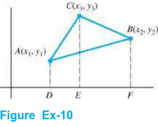
Figure Ex-25
Figure Ex-26
27.
(a) Show that if , then the reduced row-echelon form of
(b) Use part (a) to show that the system
& " ' (
28.
Find an inconsistent linear system that has more unknowns than equations.
29.
Indicate all possible reduced row-echelon forms of
(a)
(b)
30.
Discuss the relative positions of the lines , , and when (a) the system has only the trivial solution, and (b) the system has nontrivial solutions.
31.
Indicate whether the statement is always true or sometimes false. Justify your answer by giving a logical argument or a counterexample.
(a) If a matrix is reduced to reduced row-echelon form by two different sequences of elementary row operations, the resulting matrices will be different.
(b) If a matrix is reduced to row-echelon form by two different sequences of elementary row operations, the resulting matrices might be different.
(c) If the reduced row-echelon form of the augmented matrix for a linear system has a row of zeros, then the system must have infinitely many solutions.
(d) If three lines in the -plane are sides of a triangle, then the system of equations formed from their equations has three solutions, one corresponding to each vertex.
32.
Indicate whether the statement is always true or sometimes false. Justify your answer by giving a logical argument or a counterexample.
(a) A linear system of three equations in five unknowns must be consistent.
(b) A linear system of five equations in three unknowns cannot be consistent.
(c) If a linear system of n equations in n unknowns has n leading 1's in the reduced row-echelon form of its augmented matrix, then the system has exactly one solution.
(d) If a linear system of n equations in n unknowns has two equations that are multiples of one another, then the system is inconsistent.
1.3
Rectangular arrays of real numbers arise in many contexts other than as augmented matrices for systems of linear equations. In this section we begin our study of matrix theory by giving some of the fundamental definitions of the subject. We shall see how matrices can be combined through the arithmetic operations of addition, subtraction, and multiplication.In Section 1.2 we used rectangular arrays of numbers, called augmented matrices, to abbreviate systems of linear equations. However, rectangular arrays of numbers occur in other contexts as well. For example, the following rectangular array with three rows and seven columns might describe the number of hours that a student spent studying three subjects during a certain week:
Mon. Tues. Wed. Thurs. Fri. Sat. Sun.
Math 2 3 2 4 1 4 2
History 0 3 1 4 3 2 2
Language 4 1 3 1 0 0 2
If we suppress the headings, then we are left with the following rectangular array of numbers with three rows and seven columns, called a “matrix”:
More generally, we make the following definition.
D E F I N I T I O N
A matrix is a rectangular array of numbers. The numbers in the array are called the entries in the matrix.
EXAMPLE 1 Examples of Matrices
The size of a matrix is described in terms of the number of rows (horizontal lines) and columns (vertical lines) it contains. For example, the first matrix in Example 1 has three rows and two columns, so its size is 3 by 2 (written ). In a size description, the first number always denotes the number of rows, and the second denotes the number of columns. The remaining matrices in Example 1 have sizes , , , and , respectively. A matrix with only one column is called a column matrix (or a column vector), and a matrix with only one row is called a row matrix (or a row vector). Thus, in Example 1 the matrix is a column matrix, the matrix is a row matrix, and the matrix is both a row matrix and a column matrix. (The term vector has another meaning that we will discuss in subsequent chapters.)
Remark It is common practice to omit the brackets from a matrix. Thus we might write 4 rather than [4]. Although this makes it impossible to tell whether 4 denotes the number “four” or the matrix whose entry is “four,” this rarely causes problems, since it is usually possible to tell which is meant from the context in which the symbol appears.
We shall use capital letters to denote matrices and lowercase letters to denote numerical quantities; thus we might write
When discussing matrices, it is common to refer to numerical quantities as scalars. Unless stated otherwise, scalars will be real numbers; complex scalars will be considered in Chapter 10.
The entry that occurs in row i and column j of a matrix A will be denoted by . Thus a general matrix might be written as
and a general matrix as
(1)
When compactness of notation is desired, the preceding matrix can be written as
the first notation being used when it is important in the discussion to know the size, and the second being used when the size need not be emphasized. Usually, we shall match the letter denoting a matrix with the letter denoting its entries; thus, for a matrix B we would generally use for the entry in row i and column j, and for a matrix C we would use the notation . The entry in row i and column j of a matrix A is also commonly denoted by the symbol . Thus, for matrix 1 above, we have
and for the matrix
we have , , , and .
A matrix A with n rows and n columns is called a square matrix of order n, and the shaded entries , , …, in 2 are said to be on the main diagonal of A.
(2)
So far, we have used matrices to abbreviate the work in solving systems of linear equations. For other applications, however, it is desirable to develop an “arithmetic of matrices” in which matrices can be added, subtracted, and multiplied in a useful way. The remainder of this section will be devoted to developing this arithmetic.
D E F I N I T I O N
Two matrices are defined to be equal if they have the same size and their corresponding entries are equal.
In matrix notation, if and have the same size, then if and only if , or, equivalently, for all i and j.
EXAMPLE 2 Equality of Matrices
Consider the matrices
If , then , but for all other values of x the matrices A and B are not equal, since not all of their corresponding entries are equal. There is no value of x for which since A and C have different sizes.
D E F I N I T I O N
If A and B are matrices of the same size, then the sum is the matrix obtained by adding the entries of B to the corresponding entries of A, and the difference is the matrix obtained by subtracting the entries of B from the corresponding entries of A. Matrices of different sizes cannot be added or subtracted.
EXAMPLE 3 Addition and Subtraction
Consider the matrices
Then
The expressions , , , and are undefined.
D E F I N I T I O N
If A is any matrix and c is any scalar, then the product is the matrix obtained by multiplying each entry of the matrix A by c. The matrix is said to be a scalar multiple of A.
In matrix notation, if , then
EXAMPLE 4 Scalar Multiples
For the matrices
we have
It is common practice to denote by .
If , , …, are matrices of the same size and , , …, are scalars, then an expression of the form
is the linear combination of A, B, and C with scalar coefficients 2, −1, and .
Thus far we have defined multiplication of a matrix by a scalar but not the multiplication of two matrices. Since matrices are added by adding corresponding entries and subtracted by subtracting corresponding entries, it would seem natural to define multiplication of matrices by multiplying corresponding entries. However, it turns out that such a definition would not be very useful for most problems. Experience has led mathematicians to the following more useful definition of matrix multiplication.
D E F I N I T I O N
If A is an matrix and B is an matrix, then the product is the matrix whose entries are determined as follows. To find the entry in row i and column j of , single out row i from the matrix A and column j from the matrix B. Multiply the corresponding entries from the row and column together, and then add up the resulting products.
EXAMPLE 5 Multiplying Matrices
Consider the matrices
Since A is a matrix and B is a matrix, the product is a matrix. To determine, for example, the entry in row 2 and column 3 of , we single out row 2 from A and column 3 from B. Then, as illustrated below, we multiply corresponding entries together and add up these products.
The entry in row 1 and column 4 of is computed as follows:
The definition of matrix multiplication requires that the number of columns of the first factor A be the same as the number of rows of the second factor B in order to form the product . If this condition is not satisfied, the product is undefined. A convenient way to determine whether a product of two matrices is defined is to write down the size of the first factor and, to the right of it, write down the size of the second factor. If, as in 3, the inside numbers are the same, then the product is defined. The outside numbers then give the size of the product.
(3)
EXAMPLE 6 Determining Whether a Product Is Defined
Suppose that A, B, and C are matrices with the following sizes:
Then by 3, is defined and is a matrix; is defined and is a matrix; and is defined and is a matrix. The products , , and are all undefined.
In general, if is an matrix and is an matrix, then, as illustrated by the shading in 4,
(4)
the entry in row i and column j of is given by
(5)
!
Sometimes it may be desirable to find a particular row or column of a matrix product without computing the entire product. The following results, whose proofs are left as exercises, are useful for that purpose:
(6)
(7)
EXAMPLE 7 Example 5 Revisited
If A and B are the matrices in Example 5, then from 6 the second column matrix of can be obtained by the computation
and from 7 the first row matrix of can be obtained by the computation
If , , …, denote the row matrices of A and , , …, denote the column matrices of B, then it follows from Formulas 6 and 7 that
(9)
Remark Formulas 8 and 9 are special cases of a more general procedure for multiplying partitioned matrices (see Exercises 15, 16 and 17).
"
Row and column matrices provide an alternative way of thinking about matrix multiplication. For example, suppose that
Then
(10)
In words, 10 tells us that the product of a matrixAwith a column matrixxis a linear combination of the column matrices ofAwith the coefficients coming from the matrixx. In the exercises we ask the reader to show that the product of a matrixywith an matrixAis a linear combination of the row matrices ofAwith scalar coefficients coming fromy.
EXAMPLE 8 Linear Combinations
The matrix product
can be written as the linear combination of column matrices
The matrix product
can be written as the linear combination of row matrices
EXAMPLE 9 Columns of a Product as Linear Combinations
We showed in Example 5 that
The column matrices of can be expressed as linear combinations of the column matrices of A as follows:
#
$
"
Matrix multiplication has an important application to systems of linear equations. Consider any system of m linear equations in n unknowns.
Since two matrices are equal if and only if their corresponding entries are equal, we can replace the m equations in this system by the single matrix equation
The matrix on the left side of this equation can be written as a product to give
If we designate these matrices by A, x, and b, respectively, then the original system of m equations in n unknowns has been replaced by the single matrix equation
$
#
The equation with A and b given defines a linear system to be solved for x. But we could also write this equation as , where A and x are given. In this case, we want to compute y. If A is , then this is a function that associates with every column vector x an column vector y, and we may view A as defining a rule that shows how a given x is mapped into a corresponding y. This idea is discussed in more detail starting in Section 4.2.
EXAMPLE 10 A Function Using Matrices
Consider the following matrices.
The product is
so the effect of multiplying A by a column vector is to change the sign of the second entry of the column vector. For the matrix
the product is
so the effect of multiplying B by a column vector is to interchange the first and second entries of the column vector, also changing the sign of the first entry.
Figure 1.3.1
$
We conclude this section by defining two matrix operations that have no analogs in the real numbers.
D E F I N I T I O N
If A is any matrix, then the transpose ofA, denoted by , is defined to be the matrix that results from interchanging the rows and columns of A; that is, the first column of is the first row of A, the second column of is the second row of A, and so forth.
EXAMPLE 11 Some Transposes
The following are some examples of matrices and their transposes.
and column j of is the entry in row j and column i of A; that is,
(11) Note the reversal of the subscripts.
In the special case where A is a square matrix, the transpose of A can be obtained by interchanging entries that are
symmetrically positioned about the main diagonal. In 12 it is shown that can also be obtained by “reflecting” A about its main diagonal.
(12)
D E F I N I T I O N
If A is a square matrix, then the trace of A, denoted by , is defined to be the sum of the entries on the main diagonal of A. The trace of A is undefined if A is not a square matrix.
EXAMPLE 12 Trace of a Matrix
The following are examples of matrices and their traces.
Exercise Set
1.3
Click here for Just Ask!
1.
Determine which of the following matrix expressions are defined. For those that are defined, give the size of the resulting matrix.
(a)
(b)
(c)
(d)
(e)
(f)
(g)
(h)
2.
Solve the following matrix equation for a, b, c, and d.
3.
Consider the matrices
Compute the following (where possible).
(b)
(c)
(d)
(e)
(f)
(g)
(h)
(i)
(j)
(k)
(l)
4.
Using the matrices in Exercise 3, compute the following (where possible).
(a)
(b)
(c)
(d)
(e)
(g)
(h)
5.
Using the matrices in Exercise 3, compute the following (where possible).
(a)
(b)
(c)
(d)
(e)
(f)
(g)
(h)
(i)
(j)
(k)
6.
Using the matrices in Exercise 3, compute the following (where possible).
(a)
(c)
(d)
(e)
(f)
7. Let
Use the method of Example 7 to find
(a) the first row of
(b) the third row of
(c) the second column of
(d) the first column of
(e) the third row of
(f) the third column of
8.
Let A and B be the matrices in Exercise 7. Use the method of Example 9 to
(a) express each column matrix of as a linear combination of the column matrices of A
(b) express each column matrix of as a linear combination of the column matrices of B
(a) Show that the product can be expressed as a linear combination of the row matrices of A with the scalar coefficients coming from y.
(b) Relate this to the method of Example 8.
Hint Use the transpose operation.
10.
Let A and B be the matrices in Exercise 7.
(a) Use the result in Exercise 9 to express each row matrix of as a linear combination of the row matrices of B.
(b) Use the result in Exercise 9 to express each row matrix of as a linear combination of the row matrices of A.
11.
Let C, D, and E be the matrices in Exercise 3. Using as few computations as possible, determine the entry in row 2 and column 3 of .
12.
(a) Show that if and are both defined, then and are square matrices.
(b) Show that if A is an matrix and is defined, then B is an matrix.
13.
In each part, find matrices A, x, and b that express the given system of linear equations as a single matrix equation .
(a)
(b)
14.
(a)
(b)
15.
If A and B are partitioned into submatrices, for example,
then can be expressed as
provided the sizes of the submatrices of A and B are such that the indicated operations can be performed. This method of multiplying partitioned matrices is called block multiplication. In each part, compute the product by block
multiplication. Check your results by multiplying directly.
(a)
(b)
16.
Adapt the method of Exercise 15 to compute the following products by block multiplication.
(a)
(c)
17.
In each part, determine whether block multiplication can be used to compute from the given partitions. If so, compute the product by block multiplication.
Note See Exercise 15.
(a)
(b)
18.
(a) Show that if A has a row of zeros and B is any matrix for which is defined, then also has a row of zeros.
(b) Find a similar result involving a column of zeros.
19.
Let A be any matrix and let 0 be the matrix each of whose entries is zero. Show that if , then or .
20.
Let I be the matrix whose entry in row i and column j is
Show that for every matrix A.
21.
(a)
(b)
(c)
(d)
22.
Find the matrix whose entries satisfy the stated condition.
(a)
(b)
(c)
23.
Consider the function defined for matrices x by , where
Plot together with x in each case below. How would you describe the action of f?
(a)
(b)
(c)
24.
Let A be a matrix. Show that if the function defined for matrices x by satisfies the linearity property, then for any real numbers α and β and any matrices w and z.
25.
Prove: If A and B are matrices, then .
26.
Describe three different methods for computing a matrix product, and illustrate the methods by computing some product three different ways.
27.
How many matrices A can you find such that
for all choices of x, y, and z?
28.
How many matrices A can you find such that
for all choices of x, y, and z?
29.
A matrix B is said to be a square root of a matrix A if .
(a) Find two square roots of .
(b) How many different square roots can you find of ?
(c) Do you think that every matrix has at least one square root? Explain your reasoning.
30.
Let 0 denote a matrix, each of whose entries is zero.
(a) Is there a matrix A such that and ? Justify your answer.
(b) Is there a matrix A such that and ? Justify your answer.
31.
(a) The expressions and are always defined, regardless of the size of A.
(b) for every matrix A.
(c) If the first column of A has all zeros, then so does the first column of every product .
(d) If the first row of A has all zeros, then so does the first row of every product .
32.
Indicate whether the statement is always true or sometimes false. Justify your answer with a logical argument or a counterexample.
(a) If A is a square matrix with two identical rows, then AA has two identical rows.
(b) If A is a square matrix and AA has a column of zeros, then A must have a column of zeros.
(c) If B is an matrix whose entries are positive even integers, and if A is an
matrix whose entries are positive integers, then the entries of AB and BA are positive even integers.
(d) If the matrix sum is defined, then A and B must be square.
33.
Suppose the array
represents the orders placed by three individuals at a fast-food restaurant. The first person orders 4 burgers, 3 sodas, and 3 fries; the second orders 2 burgers and 1 soda, and the third orders 4 burgers, 4 sodas, and 2 fries. Burgers cost $2 each, sodas $1 each, and fries $1.50 each.
(a) Argue that the amounts owed by these persons may be represented as a function , where is equal to the array given above times a certain vector.
(c) Change the matrix for the case in which the second person orders an additional soda and 2 fries, and recompute the costs.
1.4
In this section we shall discuss some properties of the arithmetic operations on matrices. We shall see that many of the basic rules of arithmetic for real numbers also hold for matrices, but a few do not.For real numbers a and b, we always have , which is called the commutative law for multiplication. For matrices, however, AB and BA need not be equal. Equality can fail to hold for three reasons: It can happen that the product AB is defined but BA is undefined. For example, this is the case if A is a matrix and B is a matrix. Also, it can happen that AB and BA are both defined but have different sizes. This is the situation if A is a matrix and B is a matrix. Finally, as Example 1 shows, it is possible to have even if both AB and BA are defined and have the same size.
EXAMPLE 1 AB and BA Need Not Be Equal
Consider the matrices
Multiplying gives
Thus, .
Although the commutative law for multiplication is not valid in matrix arithmetic, many familiar laws of arithmetic are valid for matrices. Some of the most important ones and their names are summarized in the following theorem.
T H E O R E M 1 . 4 . 1
Properties of Matrix Arithmetic
Assuming that the sizes of the matrices are such that the indicated operations can be performed, the following rules of matrix arithmetic are valid.
(a)
(b)
(d)
(e)
(f)
(g)
(h)
(i)
(j)
(k)
(l)
(m)
To prove the equalities in this theorem, we must show that the matrix on the left side has the same size as the matrix on the right side and that corresponding entries on the two sides are equal. With the exception of the associative law in part (c), the proofs all follow the same general pattern. We shall prove part (d) as an illustration. The proof of the associative law, which is more complicated, is outlined in the exercises.
Proof (d) We must show that and have the same size and that corresponding entries are equal. To form
, the matrices B and C must have the same size, say , and the matrix A must then have m columns, so its size must be of the form . This makes an matrix. It follows that is also an matrix and, consequently, and have the same size.
Suppose that , , and . We want to show that corresponding entries of and are
equal; that is,
Remark Although the operations of matrix addition and matrix multiplication were defined for pairs of matrices, associative laws (b) and (c) enable us to denote sums and products of three matrices as and ABC without inserting any
parentheses. This is justified by the fact that no matter how parentheses are inserted, the associative laws guarantee that the same end result will be obtained. In general, given any sum or any product of matrices, pairs of parentheses can be inserted or deleted anywhere within the expression without affecting the end result.
EXAMPLE 2 Associativity of Matrix Multiplication
As an illustration of the associative law for matrix multiplication, consider
Then
Thus
and
so , as guaranteed by Theorem 1.4.1c.
A matrix, all of whose entries are zero, such as
is called a zero matrix. A zero matrix will be denoted by 0; if it is important to emphasize the size, we shall write for the zero matrix. Moreover, in keeping with our convention of using boldface symbols for matrices with one column, we will denote a zero matrix with one column by 0.
If A is any matrix and 0 is the zero matrix with the same size, it is obvious that . The matrix 0 plays much the same role in these matrix equations as the number 0 plays in the numerical equations .
If and , then . (This is called the cancellation law.)
If , then at least one of the factors on the left is 0.
As the next example shows, the corresponding results are not generally true in matrix arithmetic.
EXAMPLE 3 The Cancellation Law Does Not Hold
Consider the matrices
You should verify that
Thus, although , it is incorrect to cancel the A from both sides of the equation and write . Also, , yet and . Thus, the cancellation law is not valid for matrix multiplication, and it is possible for a product of matrices to be zero without either factor being zero.
In spite of the above example, there are a number of familiar properties of the real number 0 that do carry over to zero matrices. Some of the more important ones are summarized in the next theorem. The proofs are left as exercises.
T H E O R E M 1 . 4 . 2
Properties of Zero Matrices
Assuming that the sizes of the matrices are such that the indicated operations can be performed, the following rules of matrix arithmetic are valid.
(a)
(b)
(c)
(d) ;
!
"