Full Terms & Conditions of access and use can be found at
http://www.tandfonline.com/action/journalInformation?journalCode=ubes20
Download by: [Universitas Maritim Raja Ali Haji] Date: 12 January 2016, At: 22:51
Journal of Business & Economic Statistics
ISSN: 0735-0015 (Print) 1537-2707 (Online) Journal homepage: http://www.tandfonline.com/loi/ubes20
The Henderson Smoother in Reproducing Kernel
Hilbert Space
Estela Bee Dagum & Silvia Bianconcini
To cite this article: Estela Bee Dagum & Silvia Bianconcini (2008) The Henderson Smoother in Reproducing Kernel Hilbert Space, Journal of Business & Economic Statistics, 26:4, 536-545, DOI: 10.1198/073500107000000322
To link to this article: http://dx.doi.org/10.1198/073500107000000322
Published online: 01 Jan 2012.
Submit your article to this journal
Article views: 73
View related articles
The Henderson Smoother in Reproducing
Kernel Hilbert Space
Estela Bee D
AGUMand Silvia B
IANCONCINIDepartment of Statistics, University of Bologna, Via Belle Arti 41, 40126 Bologna, Italy
(estela.beedagum@unibo.it;silvia.bianconcini@unibo.it)
The Henderson smoother has been traditionally applied for trend-cycle estimation in the context of non-parametric seasonal adjustment software officially adopted by statistical agencies. This study introduces a Henderson third-order kernel representation by means of the reproducing kernel Hilbert space (RKHS) methodology. Two density functions and corresponding orthonormal polynomials have been calculated. Both are shown to give excellent representations for short- and medium-length filters. Theoretical and empirical comparisons of the Henderson third-order kernel asymmetric filters are made with the classical ones. The former are shown to be superior in terms of signal passing, noise suppression, and revision size. KEY WORDS: Biweight density function; Higher order kernels; Local weighted least squares; Spectral
properties; Symmetric and asymmetric weighting systems.
1. INTRODUCTION
The linear smoother developed by Henderson (1916) is the most widely applied to estimate the trend-cycle latent compo-nent in nonparametric seasonal adjustment software, such as the U.S. Bureau of the Census X11 method (Shiskin, Young, and Musgrave 1967) and its variants, the X11ARIMA (Dagum 1988) and X12ARIMA (Findley, Monsell, Bell, Otto, and Chen 1998). The study of the properties and limitations of the Hen-derson filter has been done in different contexts and attracted the attention of a large number of authors, among them, Cho-lette (1981), Kenny and Durbin (1982), Castles (1987), Dagum and Laniel (1987), Cleveland, Cleveland, McRae, and Terpen-ning (1990), Dagum (1996), Gray and Thomson (1996), Loader (1999), Dalton and Keogh (2000), Quenneville, Ladiray, and Lefrançois (2003), and Dagum and Luati (2004). However, none of these studies have approached the Henderson smoother from a reproducing kernel Hilbert space (RKHS) perspective.
A RKHS is a Hilbert space characterized by a kernel that reproduces, via an inner product, every function of the space or, equivalently, a Hilbert space of real-valued functions with the property that every point evaluation functional is a bounded linear functional.
Parzen (1959) was the first to introduce a RKHS approach to time series applying the famous Loève (1948) theorem by which there is an isometric isomorphism between the closed linear span of a second-order stationary stochastic process and the RKHS determined by its covariance function. Parzen demonstrated that the RKHS approach provides a unified framework to three fundamental problems concerning (1) least squares estimation, (2) minimum variance unbiased estimation of regression parameters, and (3) identification of unknown sig-nals perturbed by noise. Parzen’s approach is parametric, and basically consists of estimating the unknown signal by gener-alized least squares in terms of the inner product between the observations and the covariance function. A nonparametric ap-proach of the RKHS methodology was developed by DeBoor and Lynch (1966) in the context of cubic spline approxima-tion. Later, Kimeldorf and Wahba (1970) exploited both de-velopments and treated the general spline smoothing problem from a RKHS stochastic equivalence perspective. These authors
proved that minimum norm interpolation and smoothing prob-lems with quadratic constraints imply an equivalent Gaussian stochastic process.
The main purpose of this study is to introduce a nonpara-metric RKHS representation of the Henderson smoother. This Henderson kernel representation enables the construction of a hierarchy of kernels with varying smoothing properties. Fur-thermore, for each kernel order, the asymmetric filters can be derived coherently with the corresponding symmetric weights or from a lower or higher order kernel within the hierarchy, if more appropriate. In the particular case of the currently applied asymmetric Henderson filters, those obtained by means of the RKHS, coherent to the symmetric smoother, are shown to have superior properties from the viewpoint of signal passing, noise suppression, and revisions. We compare the performance of the kernel representations relative to the classical filters using real life series.
Section 2 briefly deals with the basic properties of Hilbert spaces and reproducing kernels. Section 3 discusses the classi-cal Henderson symmetric smoother and two density functions are derived to generate the corresponding third-order kernel representations. It illustrates the approximations for spans of 9, 13, and 23 terms. Section 4 presents the asymmetric Henderson kernel filters and makes a comparison with the currently be-ing used by means of spectral analysis. Section 5 illustrates the new asymmetric Henderson kernel smoothers with applications to real data. Finally, Section 6 gives the conclusions.
2. LINEAR FILTERS IN REPRODUCING KERNEL HILBERT SPACES
Let{yt,t=1,2, . . . ,N}denote the input series. In this study
we work under the following (basic) specification for the input time series.
Assumption 1. The input series{yt,t=1,2, . . . ,N}can be
decomposed into the sum of a systematic component, called the
© 2008 American Statistical Association Journal of Business & Economic Statistics October 2008, Vol. 26, No. 4 DOI 10.1198/073500107000000322
536
signal (or nonstationary mean)gt, plus an erratic componentut,
called the noise, such that
yt=gt+ut. (1)
The noiseutis assumed either to be a white noise,WN(0, σu2),
or, more generally, to follow a stationary and invertible autore-gressive moving average (ARMA) process.
If the input series{yt,t=1,2, . . . ,N}is seasonally adjusted
or without seasonality, the signalgt represents the trend and
cyclical components, usually referred to as trend-cycle for they are estimated jointly. The trend-cycle can be deterministic or stochastic, and have a global or a local representation. It can be representedlocallyby a polynomial of degreepof a variablej, which measures the distance between yt and the neighboring
observationsyt+j.
Assumption 2. Givenut for some time pointt, it is possible
to find a local polynomial trend estimator
gt(j)=a0+a1j+ · · · +apjp+εt(j), (2)
wherea0,a1, . . . ,ap∈Randεtis assumed to be purely random
and mutually uncorrelated withut.
The coefficientsa0,a1, . . . ,apcan be estimated by ordinary
or weighted least squares or by summation formulas. The solu-tion foraˆ0provides the trend-cycle estimategˆt(0), which
equiv-alently consists in a weighted average applied in a moving man-ner (Kendall, Stuart, and Ord 1983), such that
ˆ
The weights depend on (1) the degree of the fitted polyno-mial, (2) the amplitude of the neighborhood, and (3) the shape of the function used to average the observations in each neigh-borhood.
Once a (symmetric) span 2m+1 of the neighborhood has been selected, the wj’s for the observations corresponding to
points falling out of the neighborhood of any target point are null or approximately null, such that the estimates of theN−2m central observations are obtained by applying 2m+1 symmet-ric weights to the observations neighboring the target point. The missing estimates for the first and lastmobservations can be obtained by applying asymmetric moving averages of vari-able length to the first and lastmobservations, respectively. The length of the moving average or time-invariant symmetric lin-ear filter is 2m+1, whereas the asymmetric linear filters length is time varying.
whereW(B)is a linear nonparametric estimator.
Definition 1. Givenp≥2,W(B)is apth-order kernel if polynomial trend of degreep−1 without distortion.
A different characterization of apth-order nonparametric es-timator can be provided by means of the RKHS methodology.
A Hilbert space is a complete linear space with a norm given by an inner product. The space of square integrable functions L2and the finitep-dimensional spaceRpare those used in this study.
Assumption 3. The time series {yt,t=1,2, . . . ,N}is a
fi-nite realization of a family of square Lebesgue integrable ran-dom variables, that is,R|Yt|2<∞. Hence, the random process
{Yt}t∈Rbelongs to the spaceL2(R).
The spaceL2(R)is a Hilbert space endowed with the inner product defined by tion, weighting each observation to take into account its posi-tion in time. In the following,L2(R)will be indicated asL2(f0). Under Assumption 2, the local trend gt(·) belongs to the
Pp space of polynomials of degree at most p,p being a non-negative integer.
Pp is a Hilbert subspace ofL2(f
0), hence inherits its inner product given by
Corollary 1. The spacePp is a reproducing kernel Hilbert space of polynomials on some domainT ⊆R, that is, for all t∈T and for allP∈Pp, there exists an element
Rp(t; ·)∈Pp, such that P(t)= P(·);Rp(t; ·).
The proof easily follows by the fact that any finite-dimen-sional Hilbert space has a reproducing kernel (see, for details, Berlinet and Thomas-Agnan 2003).
Rp(t,·)is calledreproducing kernelbecause
R(t,·),R(·,s) =R(s,t). (9) Formally,Ris a function
R:T×T→R, (s,t) →R(s,t),
satisfying the following properties:
1. R(t,·)∈H,∀t∈T;
2. g(·),R(t,·) =g(t),∀t∈Tandg∈H.
538 Journal of Business & Economic Statistics, October 2008
This last condition is called the “reproducing property”: the value of the function gat the pointt is reproduced by the in-ner product ofgwithR(t,·). where the positive real numbermdetermines the neighborhood ofton which the deviation betweenyt+jandgt(j)is taken into
account in the L2-sense. For this reason, 2m+1 is called the bandwidth. The weighting functionf0depends on the distance between the target pointtand each observation in the 2m+1 points neighborhood (form+1≤t≤N−m).
Theorem 2. Under Assumptions 1, 2, and 3, the minimiza-tion problem (10) has a unique and explicit soluminimiza-tion.
Proof. By the projection theorem (see, e.g., Priestley 1981), each element yt+j of the Hilbert space L2(f0)can be decom-posed into the sum of its projection in a Hilbert subspace of L2(f0), such as the spacePp, plus its orthogonal complement as whereRpis the reproducing kernel of the spacePp.
Hence, the estimategˆtcan be equivalently seen as the
projec-tion ofytonPpand as a local weighted average of the
observa-tions for the discrete version of the filter given in (4), where the weightswjare derived by a kernel functionKof orderp+1,
Kp+1(t)=Rp(t,0)f0(t), (15) wherepis the degree of the fitted polynomial.
The following result, proved by Berlinet (1993), is funda-mental.
Corollary 3. Kernels of order (p+1), p≥1, can be writ-ten as products of the reproducing kernelRp(t,·)of the space
Pp⊆L2(f
0)and a density functionf0with finite moments up to order 2p. That is,
Kp+1(t)=Rp(t,0)f0(t).
Remark 1(Christoffel–Darboux formula). For any sequence
(Pi)0≤i≤pof(p+1)orthonormal polynomials inL2(f0), An important outcome of the RKHS theory is that linear filters can be grouped into hierarchies{Kp,p=2,3,4, . . .}with the
following property: each hierarchy is identified by a densityf0 and contains kernels of order 2,3,4, . . .which are products of orthonormal polynomials byf0.
The weight system of a hierarchy is completely determined by specifying (1) the bandwidth or smoothing parameter, (2) the maximum order of the estimator in the family, and (3) the den-sityf0.
There are several procedures to determine the bandwidth or smoothing parameter (for a detailed discussion see, e.g., Berlinet and Devroye 1994). In this study, however, the smooth-ing parameter is not derived by data-dependent optimization criteria, but we fixed it with the aim to obtain a kernel represen-tation of the most often applied Henderson smoothers. Kernels of any length, including infinite ones, can be obtained with the above approach. Consequently, the results discussed can be eas-ily extended to any filter length as long as the density function and its orthonormal polynomials are specified.
The identification and specification of the density is one of the most crucial tasks for smoothers based on local polynomial fitting by weighted least squares, as Loess and the Henderson smoother. The density is related to the weighting penalizing function of the minimization problem.
We remark that the RKHS approach can be applied to any linear filter characterized by varying degrees of fidelity and smoothness as described by Gray and Thomson (1996). In par-ticular, applications to local polynomial smoothers are treated in Dagum and Bianconcini (2006), and to smoothing splines in Wahba (1990).
3. THE SYMMETRIC HENDERSON SMOOTHER AND ITS KERNEL REPRESENTATION
Recognition of the fact that the smoothness of the estimated trend-cycle curve depends directly on the smoothness of the weight diagram led Henderson (1916) to develop a formula which makes the sum of squares of the third differences of the smoothed series a minimum for any number of terms. Hender-son’s starting point was the requirement that the filter should reproduce a cubic polynomial trend without distortion. Hen-derson proved that three alternative smoothing criteria give the same formula, as shown explicitly by Kenny and Durbin (1982) and Gray and Thomson (1996): (1) minimization of the vari-ance of the third differences of the series defined by the appli-cation of the moving average; (2) minimization of the sum of squares of the third differences of the coefficients of the mov-ing average formula; (3) fittmov-ing a cubic polynomial by weighted least squares, where the weights are chosen to minimize the sum of squares of their third differences.
The problem is one of fitting a cubic trend by weighted least squares to the observationsyt+j,j= −m, . . . ,m, the value of the
fitted function atj=0 being taken as the smoothed observa-tiongˆt. Representing the weight assigned to the residuals from
the local polynomial regression byWj,j= −m, . . . ,m, where
where the solution for the constant termaˆ0is the smoothed ob-servationgˆt. Henderson (1916) showed thatgˆtis given by
ˆ
whereφ (j)is a cubic polynomial whose coefficients have the property that the smoother reproduces the data if they follow a cubic. Henderson also proved the converse: if the coefficients of a cubic-reproducing summation formula{wj,j= −m, . . . ,m}
do not change their sign more than three times within the fil-ter span, then the formula can be represented as a local cubic smoother with weights Wj>0 and a cubic polynomial φ (j),
such thatφ (j)Wj=wj. Henderson (1916) measured the amount
of smoothing of the input series by(3y
t)2or equivalently
by the sum of squares of the third differences of the weight diagram,
(3wj)2. The solution is that resulting from the
minimization of a cubic polynomial function by weighted least squares with
Wj∝ {(m+1)2−j2}{(m+2)2−j2}{(m+3)2−j2} (20)
as the weighting penalty function of criterion (3) above. Follow-ing Henderson (1916), the weight diagram{wj,j= −m, . . . ,m}
corresponding to (20), known as Henderson’s ideal formula, is obtained, for a filter length equal to 2m′−3, by
wj=315[(m′−1)2−j2](m′2−j2)
× [(m′+1)2−j2](3m′2−16−11j2)
8m′(m′2−1)(4m′2−1)(4m′2−9)(4m′2−25). (21) This optimality result has been rediscovered several times in modern literature, usually for asymptotic variants. Loader (1999) showed that Henderson’s ideal formula (21) is a finite sample variant of a kernel with second-order vanishing mo-ments which minimizes the third derivative of the function given by Müller (1984). In particular, Loader showed that for largem, the weights of Henderson’s ideal penalty functionWj
are approximatelym6W(j/m), where W(j/m)is the triweight function. He concluded that, for very large m, the weight di-agram is approximately (315/512)∗W(j/m)(3−11(j/m)2)
equivalent to the kernel given by Müller (1984).
To derive the Henderson kernel hierarchy by means of the RKHS methodology, the density corresponding toWj and its
orthonormal polynomials have to be determined.
The triweight density function gives very poor results when the Henderson smoother spans are of short or medium lengths, as in most application cases, ranging from 5 to 23 terms. Hence, we derive the exact density function corresponding toWj.
Theorem 4. The exact probability density corresponding to Henderson’s ideal weighting penalty function (20) is given by
f0H(t)=
(m+1)
k W((m+1)t), t∈ [−1,1], (22) wherek=m+1
−m−1W(j)djandj=(m+1)t.
Proof. Interpolating the weighting function (20), we can note thatW(j)is nonnegative in the intervals(−m−1,m+1), the positive definite condition. The integralk=m+1
−m−1W(j)dj is different from 1 and represents the integration constant on this support. It follows that the density corresponding toW(j)
on the interval[−m−1,m+1]is given by f0(j)=W(j)/k.
To eliminate the dependence of the support on the bandwidth parameterm, a new variable ranging on[−1,1],t=j/(m+1), is considered. Applying the change of variables method,
f0H(t)=f0(t−1(j)) filter is the classical 13-term Henderson and the corresponding probability function results: Following Corollary 3, to obtain higher order kernels the cor-responding orthonormal polynomials have to be computed for the density (22). The polynomials can be derived by the Gram– Schmidt orthonormalization procedure or by solving the Han-kel system based on the moments of the densityf0H
(Brezin-ski 1980). This latter is the approach followed in this study. The hierarchy corresponding to the 13-term Henderson kernel is shown in Table 1, where forp=3 it provides a representation of the classical Henderson filter.
Because the triweight density function gives a poor approx-imation of the Henderson weights for smallm(5 to 23 terms), we search for another density function with well-known theo-retical properties. The main reason is that the exact density (22) is a function of the bandwidth and needs to be calculated any time thatmchanges together with its corresponding orthonor-mal polynomials. We found the biweight to give almost equiv-alent results to those obtained with the exact density function without the need to be calculated any time that the Henderson smoother length changes.
Another important advantage is that the biweight density function belongs to the well-known Beta distribution family, that is,
540 Journal of Business & Economic Statistics, October 2008
Table 1. 13-term Henderson kernel hierarchy
Henderson kernels Kernel orders function. The orthonormal polynomials needed for the repro-ducing kernel associated to the biweight function are the Jacobi polynomials, for which explicit expressions for computation are available, and their properties have been widely studied in liter-ature.
Therefore, we obtain another Henderson kernel hierarchy us-ing the biweight density
combined with the Jacobi orthonormal polynomials. These latter are characterized by the following explicit expression (Abramowitz and Stegun 1972):
The Henderson second-order kernel is given by the density function f0B, because the reproducing kernel R1(j,0) of the space of polynomials of degree at most 1 is always equal to 1. On the other hand, the third-order kernel is given by
15
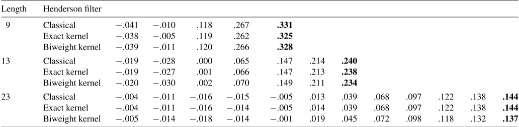
In Table 2 we give the classical and the two kernel Henderson symmetric weights for spans of 9, 13, and 23 terms, where the central weight values are shown in bold. Figure 1 illustrates the 13-term Henderson smoothers.
The small discrepancy of the two kernel functions relative to the classical Henderson smoother are due to the fact that the ex-act density is obtained by interpolation from a finite small num-ber of points of the weighting penalty functionWj. On the other
hand, the biweight is already a density function which is made discrete by choosing selected points to produce the weights. We
also calculated the smoothing measure
(3wj)2for each
fil-ter span as shown in Table 3.
The smoothing powers of the filters are very close except for the exact 9-term Henderson kernel which gives the smoothest curve.
Given the “virtual” equivalence for symmetric weights, we use the RKHS methodology to generate the correspondent asymmetric filters for themfirst and last points.
4. ASYMMETRIC HENDERSON SMOOTHERS AND THEIR KERNEL REPRESENTATIONS
The asymmetric Henderson smoothers currently in use were developed by Musgrave (1964a,b). They are based on the min-imization of the mean squared revision between the final esti-mates (obtained by the application of the symmetric filter) and the preliminary ones (obtained by the application of an asym-metric filter) subject to the constraint that the sum of the weights is equal to 1 (see, e.g., Doherty 2001). The assumption made is that at the end of the series, the seasonally adjusted values fol-low a linear trend-cycle plus a purely random irregularεt, such
thatεt∼IID(0, σ2).
The asymmetric weights of the Henderson kernels are de-rived by adapting the third-order kernel functions to the length of the lastmasymmetric filters such that
wj=
K(j/b)
q
i=−mK(i/b)
, j= −m, . . . ,q, (28)
where we denote withK(·)the third-order Henderson kernel, jthe distance to the target pointt,bthe bandwidth parameter equal tom+1, and m+q+1 the asymmetric filter length. For example, the asymmetric weights of the 13-term Henderson kernel for the last point are given by
wj=
K(j/7)
0
i=−6K(i/7)
, j= −6, . . . ,0. (29)
Table 2. Weight systems for 9-, 13-, and 23-term Henderson smoothers
Length Henderson filter
Figure 1. Classical Henderson smoothers and third-order Henderson kernels of 13 terms (—– classical Henderson;· · · biweight kernel; –+– exact kernel).
Figure 2 shows the gain functions of the symmetric Hender-son smoother together with the classical and kernel representa-tion for the last point superposed on the X11/X12ARIMA sea-sonal adjustment (SA) symmetric filter. This latter results from the convolution of (1) 12-term centered moving average (MA), (2) 3×3 MA, (3) 3×5 MA, and (4) 13-term Henderson MA. Its property has been widely discussed in Dagum, Chaab, and Chiu (1996). The gain function of the SA filter should be in-terpreted as relating the spectrum of the original series to the spectrum of the estimated seasonally adjusted series.
It is apparent that the asymmetric Henderson kernel filter does not amplify the signal as the classical asymmetric one and converges faster to the final one. Furthermore, the asymmetric kernel suppresses more noise relative to the Musgrave filter. Be-cause the weights of the biweight and exact Henderson kernels are equal up to the third digit, no visible differences are seen in the corresponding gain and phaseshift functions. Hence, we only show those corresponding to the exact Henderson kernel in Figures 2 and 3.
There is an increase of the phase shift for the low frequencies relative to that of the classical 13-term Henderson but both are less than a month, as exhibited in Figure 3.
5. EMPIRICAL ANALYSIS
We apply the classical and kernel Henderson smoothers for the last point to a set of 30 series selected from the Federal
Table 3. Sum of squares of the third differences of the weights for the classical and kernel Henderson smoother
Filters 9-term 13-term 23-term
Classical Henderson smoother .053 .01 .00
Exact Henderson kernel .048 .01 .00
Biweight Henderson kernel .052 .01 .00
Reserve Bank of St. Louis. These series are the most impor-tant concerning socioeconomic indicators and they have been taken in seasonally adjusted form. The periods chosen vary to sufficiently cover the various lengths published for these series. For each series we calculate the differences between their cor-responding absolute percentage revisions (APR) defined by
Difference in the APR
= Xˆ
C t − ˆXtCF
ˆ
XtCF − ˆ
XtK− ˆXKFt ˆ XtKF
×100
∀t=1,2, . . . ,N, (30) where XˆtC and XˆKt denote the trend-cycle estimates at time t obtained by the Henderson and kernel asymmetric filters, re-spectively,XˆCFt andXˆtKF are their final trend-cycle estimates, andNis the number of observations. The results shown in Ta-ble 4 indicate that the mean of the APR differences is always positive, hence the Henderson kernel last point predictor has smaller APR than the classical one. We also included the min-imum and maxmin-imum difference values for each series where the maximum indicates that the Henderson kernel is to be pre-ferred. The values show that the latter is systematically much greater than its corresponding minimum. In view of these ex-cellent results, we would recommend the replacement of the current Musgrave filters by the kernel ones in seasonal adjust-ment software.
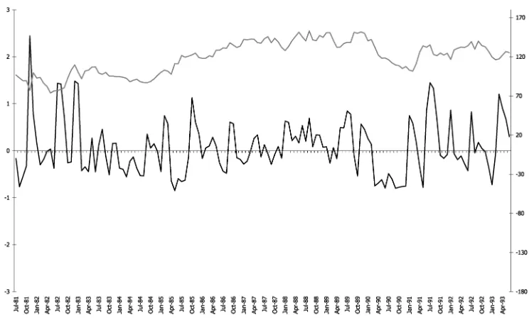
We now illustrate how the “reproducing” Henderson kernel estimator responds to the variability of the data by means of two series characterized by different levels of noise-to-signal ratios. The first series, House Spending Index (HSI), is one of the Canadian leading indicators discussed in Dagum (1996). This series covers the period January 1981–December 1993 and is published by Statistics Canada, in both original and seasonally adjusted forms. TheI/Cratio (noise over signal) for this series, calculated by the X11/X12ARIMA software, is equal to 1.77 and hence, falls within the range where a 13-term Henderson is
542 Journal of Business & Economic Statistics, October 2008
Figure 2. Gain functions of the (last point) asymmetric 13-term filter (—) and kernel ( ) with the corresponding symmetric (– – –) and SA cascade filter (· · ·).
chosen for trend-cycle estimation. The HSI signal is dominated by relative short cycles, where according to the gain functions shown in Figure 2 there should be an advantage for the kernel asymmetric filter. We produce the trend-cycle estimates of the series applying the asymmetric last point filters of both classical and kernel Henderson representation together with the symmet-ric one.
To compare the performances of the two asymmetric smoothers, in Figure 4 we superposed the temporal pattern of the APR differences together with the original data. The tem-poral pattern of the APR differences clearly favors the kernel asymmetric filter for the period September 1981–July 1983 and from May 1990 up to the end of the series. These two periods are characterized by the presence of short cycles and several points of maxima and minima. The revisions differences os-cillate between −.85 and 2.45, reaching the highest values at
turning points. From August 1983 to April 1990, the series is characterized by an increasing steady trend with small fluctua-tions; hence the performances of the two filters are quite similar with the difference ranging around.50.
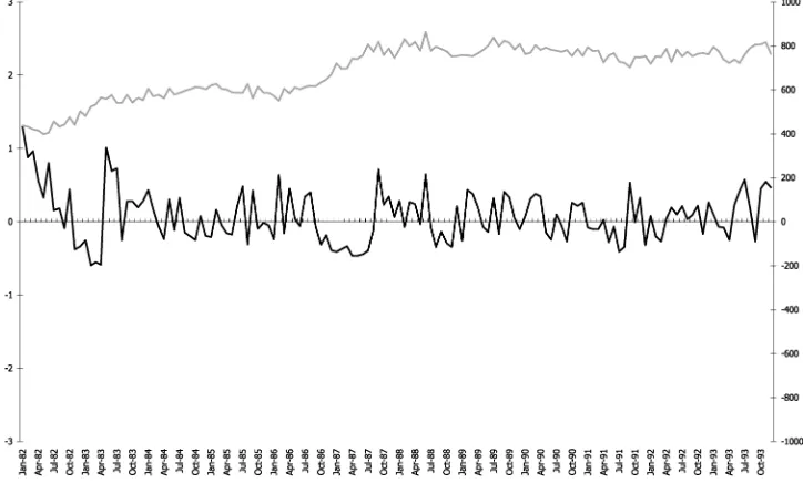
The other series, U.S. Unemployed Women, 16–19 years old, covers the period July 1981–June 1994. The original input for both trend-cycle estimators is the seasonally adjusted series modified by extreme values with zero weights as suggested by Dagum (1996). TheI/Cratio for the series is equal to 3.04 and again the 13-term Henderson is chosen, but as shown in Fig-ure 5 the trend is dominated by long-term periodic components. The high value of theI/Cratio is mainly due to the irregulars. In this case, the kernel filter still performs better than the clas-sical Henderson given its noise reduction at the high-frequency band, but the values oscillate between−.60 and 1.31 all along the series.
Figure 3. Phase shifts of the asymmetric (end point) weights of the Henderson kernel (· · ·) and of the classical H13 filter (—).
Table 4. Some statistics values of the APR differences between classical and kernel Henderson last point filters
Series Period Mean St. Dev. Min Max
U.S. TRADE AND INTERNATIONAL TRANSACTIONS
Goods and services 07/92–02/06 .01 1.23 −2.72 5.55
Goods 07/92–02/06 .03 .65 −1.57 2.42
Services 07/92–02/06 .09 .64 −1.92 2.13
Exports of goods 01/93–12/02 .05 .26 −.59 .81
Imports of goods 01/93–12/02 .03 .29 −.46 .82
Exports of services 01/93–12/02 .07 .21 −.28 .79
Imports of services 01/95–12/04 .02 .24 −.41 .73
EXCHANGE RATES
Canada/U.S. 01/90–12/99 .02 .15 −.32 .39
Japan/U.S. 01/90–12/99 .04 .54 −1.13 1.74
U.S./U.K. 01/95–12/04 .04 .54 −1.72 2.23
U.S. BANKING
1-year treasury constant maturity rate 01/93–12/03 .01 .98 −2.43 3.36
Bank prime loan rate 07/92–07/02 .06 1.18 −3.00 3.50
Travelers checks outstanding 01/91–12/00 .01 .17 −.29 .34
Other securities at all commercial banks 01/90–12/99 .03 .42 −.94 1.62
Demand deposits at commercial banks 01/95–12/04 .08 .26 −.39 .87
Savings deposits—total 01/90–12/99 .08 .21 −.29 .55
U.S. EMPLOYMENT AND POPULATION
Civilian unemployed—less than 5 weeks 01/96–12/05 .06 .34 −.83 .87
Median duration of unemployment 01/96–12/05 .02 .50 −1.00 1.30
Unemployed: 16 years and over 01/96–12/05 .01 .24 −.38 .55
U.S. unemployment women (ages 16–21) 07/81–06/94 .07 .35 −.60 1.31
CANADIAN LEADING INDICATORS
Household spending index 07/81–06/93 .07 .58 −.85 2.45
New order for durable goods 07/80–06/92 .03 .36 −.68 1.07
Average weekly hours in manufacturing 07/80–06/92 .03 .09 −.12 .19
U.S. ECONOMIC DATA
Lightweight vehicle sales: autos and light trucks 07/76–03/06 .14 .47 −1.17 2.61
Housing starts: total 01/94–12/03 .08 .39 −.89 1.16
Manufacturers’ new order 01/92–12/00 .01 .23 −.47 .53
Retail and food services sales 01/94–12/03 .02 .11 −.18 .78
Capacity utilization: manufacturing (NAICS) 01/90–12/99 .03 .13 −.28 .41
ISI manufacturing: PMI composite index 07/91–07/00 .14 1.23 −1.98 3.86
Capacity utilization: total industry 01/91–12/00 .01 .21 −.63 .73
Figure 4. House Spending Index (HSI) original series ( ) and APR differences (—).
544 Journal of Business & Economic Statistics, October 2008
Figure 5. U.S. unemployment women (age 16–19) original series ( ) and APR differences (—–).
6. CONCLUSIONS
We introduced a new representation of the Henderson smoother by means of the reproducing kernel Hilbert space (RKHS) methodology. The linear estimator is first transformed into a second-order kernel and from it a hierarchy is constructed that includes higher order kernels. We showed that the biweight density function is very close to the exact density calculated on the basis of the Henderson weighting penalty function. The bi-weight has a computing advantage over the latter, in the sense that it does not need to be calculated any time that the Hen-derson smoother length changes, as happens with the exact one. Another advantage is that the biweight density function belongs to the well-known Beta distribution family, where the associated orthonormal polynomials are the Jacobi ones. We used both densities and associated orthonormal polynomials to generate Henderson kernels of order 2 and 3. The symmetric Henderson kernel weights for both generating density functions are very close for short spans and we illustrated those most of-ten applied to monthly data.
The asymmetric weights of the Henderson kernels have been derived by adapting the third-order kernel functions to the length of the last six asymmetric filters. Applied to a set of 30 real series, the absolute percentage revisions (APR) of the last point filter are systematically smaller for the kernel representa-tion than for the classical Henderson. These results conform to their respective gain functions.
ACKNOWLEDGMENTS
We thank very much the joint editor, Arthur Lewbel, an anonymous associate editor, and two anonymous referees for their thorough reading and insightful comments to an earlier version of the paper.
[Received August 2006. Revised March 2007.]
REFERENCES
Abramowitz, M., and Stegun, I. (1972),Handbook of Mathematical Functions With Formulas, Graphs and Mathematical Tables, Washington, DC: U.S. Government Printing Office.
Berlinet, A. (1993), “Hierarchies of Higher Order Kernels,”Probability Theory and Related Fields, 94, 489–504.
Berlinet, A., and Devroye, L. (1994), “A Comparison of Kernel Density Esti-mates,”Publications de l’Institut de Statistique de l’Université de Paris, 38, 3–59.
Berlinet, A., and Thomas-Agnan, C. (2003), Reproducing Kernel Hilbert Spaces in Probability and Statistics, Amsterdam: Kluwer Academic. Brezinski, C. (1980),Pade Approximation and General Orthogonal
Polynomi-als, Basel: Birkhäuser.
Castles, I. (1987), “A Guide to Smoothing Time Series Estimates of Trend,” Catalogue No. 1316, Australian Bureau.
Cholette, P. A. (1981), “A Comparison of Various Trend-Cycle Estimators,” in
Time Series Analysis, eds. O. D. Anderson and M. R. Perryman, Amsterdam: North-Holland, pp. 77–87.
Cleveland, R., Cleveland, W., McRae, J., and Terpenning, I. (1990), “STL: A Seasonal Trend Decomposition Procedure Based on LOESS,”Journal of Official Statistics, 6, 3–33.
Dagum, E. B. (1988), “The X11ARIMA/88 Seasonal Adjustment Method— Foundation and User’s Manual,” research paper, Time Series Research and Analysis Division, Ottawa: Statistics Canada.
(1996), “A New Method to Reduce Unwanted Ripples and Revisions in Trend-Cycle Estimates From X11ARIMA,”Survey Methodology, 22, 77–83. Dagum, E. B., and Bianconcini, S. (2006), “Local Polynomial Trend-Cycle Pre-dictors in Reproducing Kernel Hilbert Spaces for Current Economic Analy-sis,”Anales de Economia Aplicada, XX, 1–22.
Dagum, E. B., and Laniel, N. (1987), “Revisions of Trend-Cycle Estimators of Moving Average Seasonal Adjustment Methods,”Journal of Business & Economic Statistics, 5, 177–189.
Dagum, E. B., and Luati, A. (2004), “Relationship Between Local and Global Nonparametric Estimators Measures of Fitting and Smoothing,”Studies in Nonlinear Dynamics and Econometrics, 8, article 17.
Dagum, E. B., Chaab, N., and Chiu, K. (1996), “Derivation and Properties of the X11ARIMA and Census X11 Linear Filters,”Journal of Official Statistics, 12, 329–348.
Dalton, P., and Keogh, G. (2000), “An Experimental Indicator to Forecast Turn-ing Points in the Irish Business Cycle,”Journal of the Statistical and Social Inquiry Society of Ireland, 29, 117–176.
DeBoor, C., and Lynch, R. (1966), “On Splines and Their Minimum Proper-ties,”Journal of Mathematics and Mechanics, 15, 953–969.
Doherty, M. (2001), “The Surrogate Henderson Filters in X11,”Australian and New Zealand Journal of Statistics, 43, 385–392.
Findley, D., Monsell, B., Bell, W., Otto, M., and Chen, B. (1998), “New Ca-pabilities and Methods of the X12ARIMA Seasonal Adjustment Program,”
Journal of Business & Economic Statistics, 16, 127–152.
Gray, A., and Thomson, P. (1996), “Design of Moving-Average Trend Filters Using Fidelity and Smoothness Criteria,” inTime Series Analysis, Vol. 2 (in memory of E. J. Hannan), eds. P. M. Robinson and M. Rosenblatt,Springer Lecture Notes in Statistics, Vol. 15, New York: Springer, pp. 205–219. Henderson, R. (1916), “Note on Graduation by Adjusted Average,”Transaction
of Actuarial Society of America, 17, 43–48.
Kendall, M. G., Stuart, A., and Ord, J. (1983),The Advanced Theory of Statis-tics, Vol. 3, London: C. Griffin, eds.
Kenny, P., and Durbin, J. (1982), “Local Trend Estimation and Seasonal Adjust-ment of Economic and Social Time Series,”Journal of the Royal Statistical Society, Ser. A, 145, 1–41.
Kimeldorf, G., and Wahba, G. (1970), “Splines Functions and Stochastic Processes,”Sankhy¯a, Ser. A, 32, 173–180.
Loader, C. (1999),Local Regression and Likelihood, New York: Springer. Loève, M. (1948), “Fonctions alèatories du second ordre,” Appendix to
Le-vy, P., Processus Stochastiques et Movement Brownien, Paris: Gauthier-Villars.
Müller, H. G. (1984), “Smooth Optimum Kernel Estimators of Regression Curves, Densities and Modes,”The Annals of Statistics, 12, 766–774.
Musgrave, J. (1964a), “A Set of End Weights to End All End Weights,” working paper, Washington, DC: U.S. Bureau of the Census.
(1964b), “Alternative Sets of Weights for Proposed X-11 Seasonal Fac-tor Curve Moving Averages,” working paper, Washington, DC: U.S. Bureau of the Census.
Parzen, E. (1959), “Statistical Inference on Time Series by Hilbert Space Meth-ods,” Technical Report 53, Stanford University, Statistics Dept.
Priestley, M. B. (1981),Spectral Analysis and Time Series, New York: Acad-emic Press.
Quenneville, B., Ladiray, D., and Lefrançois, B. (2003), “A Note on Musgrave Asymmetrical Trend-Cycle Filters,”International Journal of Forecasting, 19, 727–734.
Shiskin, J., Young, A., and Musgrave, J. (1967), “The X-11 Variant of the Cen-sus Method II Seasonal Adjustment Program,” Technical Paper 15, Washing-ton, DC: U.S. Department of Commerce, Bureau of the Census.
Wahba, G. (1990),Spline Models for Observational Data, Philadelphia: Society for Industrial and Applied Mathematics.