1845–93
Vito Antonio Muscatelli,University of Glasgow Franco Spinelli,Universita’ di Brescia
1. INTRODUCTION
There is a growing international literature on the determinants of long-run interest rates in the OECD economies (seeinter alia
Friedman and Schwartz, 1982; Summers, 1983, 1986; Barro, 1987; Barsky, 1987; Evans, 1987; Mankiw, 1987; Boudoukh and Richard-son, 1993). However, this literature has neglected the experience of Italy.1Italy’s experience is of interest because it has been more inflation prone than the other G7 countries, and has suffered from recurring fiscal deficits. It is, therefore, a natural testing ground for some of the main theories of interest rate determination.
We focus on two issues in particular. First, we examine whether nominal interest rates have fully incorporated inflationary expec-tations (the “Fisher effect”) in an environment where inflation has been high and persistent. Second, we estimate the impact of fiscal policy on real interest rates in an attempt to verify the
Address correspondence to V. A. Muscatelli, University of Glasgow, Department of Political Economy, Adam Smith Bldg., Glasgow G12 8RT, UK.
Earlier versions of this paper were presented at the Brescia Seminar on Monetary History and the History of Monetary Thought, May 1995, and the Konstanz Seminar on Monetary Theory, May 1996. We are grateful to conference participants, and in particular Giuseppe Bertola, Michael Bordo, Bill Dewald, Clements Kool, David Laidler, Jacques Melitz, Allan Meltzer, Patrick Minford, Alessandro Missale, Manfred Neumann, Anna Schwartz, Jack Tatom, Giuseppe Tullio, Jurgen Von Hagen, Axel Weber, and Jurgen Wolters for useful comments. The usual disclaimer applies. The research was completed while the first author was a visiting Professor at the Universita’ degli Studi di Bari. Muscatelli also wishes to thank the Comitato Economisti per Brescia for their generous research funding.
1With the exception of Muscatelli and Spinelli (1996), who compare the evidence on
the Gibson Paradox in the United States, United Kindgom, and Italy.
Journal of Policy Modeling22(2):149–169 (2000)
2000 Society for Policy Modeling 0161-8938/00/$–see front matter
neoclassical model of fiscal policy. The latter issue is of particular interest, given the dramatic budgetary imbalances experienced by Italy over the last few decades. The period post-1970 warrants investigation because it represents a period of sustained fiscal expansion accompanied first by an accommodating monetary pol-icy and, from the mid-1980s onwards, increasing monetary re-straint.
Our key results are as follows. First, a significant Fisher effect is only detectable in the post-World War II period. Second, we find that temporary increases in government spending have a significant impact on real interest rates, as predicted by neoclassi-cal theories of fisneoclassi-cal policy. However, debt is also found to affect the real interest rate in the late 1980s, which suggests that Ricar-dian equivalence does not hold.
This paper is structured as follows. In Section 2, we take a preliminary look at the behavior of interest rates in Italy over the last 150 years,2and provide a brief outline of the main changes in fiscal and monetary policy over this period. In Sections 3 and 4 we present some formal econometric evidence on the behavior of interest rates in Italy. Tests of the Fisher effect are reported in Section 3, and the responsiveness of real interest rates to fiscal policy is examined in Section 4. Section 5 concludes.
2. INTEREST RATES AND PRICES IN THE LONG RUN
2A. A Graphical and Statistical Summary
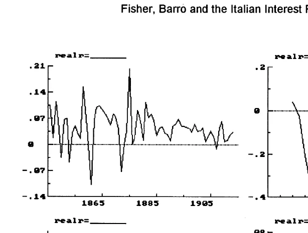
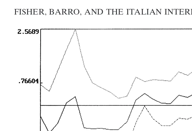
Our interest rate data consists of a long-term rate, Rwhich is the yield (net of taxes) on the long-term government bonds for the whole sample 1845–1993. The price series used for our study is a cost-of-living index, which is consistent for the whole sample period. The series employed are reported in Spinelli and Fratianni (1991), and have been extended using national data sources. The difference between the long rate (R) and the rate of change of the price variable (P) is shown in Figure 1 for various subperiods, including the war years.3
2Our data refers to the unified Italian state post-1860, and to its immediate precursor,
the Kingdom of Sardinia (Piedmont) for the period 1845–59.
3To avoid confusion later in the paper, we do not refer to R-Pas the real interest rate,
Figure 1. The gap between long rates and Inflation in Italy 1845–1993.
Table 1: Means and Standard Deviations of Interest Rates and Inflation for Various Subperiods of the Sample
Date R P R-P
1891–1900 4.4 20.5 4.9
(0.3) (0.8) (1.0)
1901–10 3.9 1.0 2.9
(0.1) (2.2) (2.2)
1911–20 4.1 15.0 210.9
(0.4) (17.4) (17.0)
1921–30 4.9 2.3 2.6
(0.3) (8.5) (8.6)
1931–40 5.0 2.4 2.6
(0.6) (8.2) (7.8)
1941–50 6.0 62.6 256.6
(0.4) (104.4) (104.1)
1951–60 6.3 3.5 2.7
(0.6) (2.7) (2.6)
1961–70 5.7 3.9 1.8
(0.8) (2.0) (2.1)
1971–80 10.9 14.2 23.2
(3.3) (5.6) (3.8)
1981–93 13.5 8.3 5.2
(3.6) (4.2) (0.9)
In Table 1 we report the means and standard deviations (in brackets) of the three key variables for various subsamples. The two World Wars and the 1970s are characterized by negative values of R-P. Up to 1913 and during the 1980s, the gap between nominal interest rates and inflation was positive, and often large by international standards.
2B. Monetary and Fiscal Regimes—A Brief Survey
Italian political unification took place gradually through a pro-cess of annexation and the acquisition of new territories on the part of the small Kingdom of Sardinia (consisting mainly of Pied-mont and adjoining territories). The Kingdom of Sardinia became the Kingdom of Italy in 1860, and unification of the whole Italian peninsula wac completed in 1970. Our sample partly covers a period prior to unification, 1845–59, where the data refers to the Kingdom of Sardinia. Post-1860 data refers to the Kingdom of Italy.
The creation of the first monetary issuing authorities in the Kingdom of Sardinia took place between 1844 and 1849. At first the issuing authorities, the Banca di Genova and the Banca di Torino4(these were merged into a single issuing bank in 1849—the Banca Nazionale degli Stati Sardi) issued notes that were fully vertible in specie. However, the first difficulties in maintaining con-vertibility were encountered in 1848 when, following an increase in military expenditures, the issuing banks were authorized to enact a loan to the Treasury and to suspend convertibility until 1851.
The next suspension of convertibility came in 1859–60 during the next phase of the struggle for unification. During the 1860s the links between the issuing authorities and the Treasury were formalized, so that bank notes could be issued to meet the demands of the state over and above the issuing banks’ reserve requirements and legal maximum circulation limits.5 A further suspension of convertibility came in 1866. It was triggered by an expansionary fiscal policy due to the expenditures incurred in the war with Austria.
A slow process of fiscal retrenchment in the 1870s eventually allowed Italy to return to full convertibility in 1880. However,
4The account presented here is brief for reasons of space. A full history of the creation
and merger of the various monetary issuing authorities in Italy can be found in Spinelli and Fratianni (1991).
5Another complication that hampered monetary control is that, following the gradual
this return to the Gold Standard was short lived. Following a combination of domestic inflationary pressures and the drying up of capital inflows, the Lira came under pressure in the mid-1880s. What followed was a de facto suspension of convertibility from the mid-1880s, as the issuing authorities refused to convert paper money. This was eventually matched by ade jure suspension of convertibility in 1893. Monetary stability was slowly restored in the period 1894–1913, but without a formal return to the Gold Standard. De facto, exchange rates were stabilized during the period 1902–13, through more prudent fiscal and monetary poli-cies.
Overall, the period 1845–1913 saw a very mixed participation to the Gold Standard, but this did not prevent a reasonably prudent monetary and fiscal stance, with average inflation at 0.8 percent (see Table 1). In general, after each exit from the Gold Standard, monetary and fiscal policies were aimed at returning within a reasonable time frame to the Standard, albeit at a lower parity. Thus, R-P was relatively high on average (4.6%), and higher than those of the main world financial centers (e.g., the United Kingdom).
From 1914 onwards, there are three major episodes of fiscal deficits: before and during the two World Wars, and during the period of increasing fiscal expansion post-1960. From the end of Bretton Woods in 1971 until the birth of the European Monetary System in 1979 there was also a gap in external exchange rate discipline. This allowed monetary policy to accommodate fiscal policy, and led to increasing inflationary pressures. Post-1979, real interest rates returned to much higher and stable levels (R-Pwas 5.1% on average), with inflation in the 1980s much lower on average (9.2%) than in the 1970s (14.2%). This resulted from a combination of three factors. First, Italy’s entry into the European exchange rate system in 1979; second, a progressive decoupling of monetary policy from fiscal policy, starting in 1981 through the removal of the obligation on the part of the Bank of Italy to purchase unsold Treasury Bills at auction; and finally, the gradual removal of capital controls, which required a partial convergence with world interest rates.
3. ECONOMETRIC EVIDENCE ON THE FISHER EFFECT AND THE DETERMINATION OF NOMINAL INTEREST RATES
Tests of the Fisher hypothesis (see Fisher, 1930),6 can be grouped into two broad categories. First, direct estimates of the Fisher equation of the type (Eq. 1):
Rt5 r 1 bE(Pt|Vt21)1ut (1)
where test b 51, where r is the real interest rate, and Vis the information set at timet21. The equation may be estimated either using the errors-in-variables methods, or the two-stage estimation methods where the expected inflation rate is modeled using infor-mation available to economic agents at timet21. Studies such as Summers (1983, 1986) fall into this category.7One of the prob-lems with such an approach is that normallyris treated as constant, so that the results are conditional on this heroic assumption. The problems are compounded by the fact that, in many cases, we might find that bothR(and implicitly r) are nonstationary over some periods, while P is integrated of degree zero [I(0)] (see Rose, 1988).
To avoid such problems, a second strand of this literature has focused on whether the inflation expectations implicit in the term structure of interest rates (see MacDonald and Murphy, 1989; Wallace and Warner, 1993) are consistent with the Fisher hypothesis.
Unfortunately in our current study we do not have a data set on the term structure that allows us to take the latter approach,8 so we have chosen the first approach, based on equation (1) and dynamic variants of this model. We first estimated equation 1 as it stands, using the errors-in-variables approach, with the realized value of current inflation as a regressor, and variables that are in the economic agents’ information set (lagged values of inflation, foreign inflation) as instruments. This has the advantage over the two-stage procedure of producing consistent standard error estimates (see Pesaran, 1987). To examine the evolution of the
6On the origins of the Fisher effect see Humphrey (1993).
7Summers (1983, 1986) uses band-spectrum regressions to verify the hypothesis. This
has the advantage of focusing on the long-run movements in the series. We take a similar approach when applying cointegration methods below.
8Most of the available short-term interest rates were administered rates during much
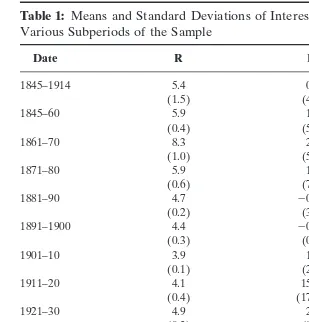
Figure 2. Coefficient on the inflation variable and standard error bands.
Fisher effect over time, we estimated equation 1 as a rolling regres-sion, using a 30 observation window. The estimated coefficient on the inflation variable b and its two-times-standard error bands are shown in Figure 2. There are several points to note about these results.
First, for the regression using post-World War II data up to the early 1970s, the coefficient is closer to unity, although always significantly less than 1. This is a result similar to that obtained for the United States by Summers (1986), who found that the 1954–71 period corresponded most closely to the Fisher hypothe-sis. One reason why the coefficient is likely to fluctuate over time is, of course, the presence of regime shifts, which implies that the hypothesis only holds in the long run (Summers, 1983). Thus, it took some time for inflationary expectations to be built into nomi-nal rates following the higher post-1970 inflation regime, and the Fisher coefficient for the final periods of the sample are conse-quently lower. This possibility is examined below.
Second, there seems little evidence for the presence of the Fisher effect in the pre-World II period. Closer inspection of the inflation series suggests that inflation in Italy in the interwar period9 is
9In the pre-1914 period, as for the United States and the United Kingdom, it is more
forecastable using a restricted ARMA(1,3) model. The inability to capture the Fisher effect before World War II is probably due to a failure of the simplest application of the rational expectations hypothesis. As noted by Barsky and De Long (1991), simple re-gression models of inflationary expectations and the Fisher hy-pothesis do not take into account the uncertainty that economic agents face in forming inflationary expectations at a time when inflation does not display any clear trends, and when sudden re-gime shifts are possible. Overall, it seems clear that expected inflation was equal to zero over the pre-World War II sample.
Third, it may be difficult for such a simple model to discriminate between increases in nominal rates in the 1980s due to the incorpo-ration of inflationary expectations, and positive effects on the real interest rate due to the expansionary fiscal policy in Italy over the last 2 decades.
As a further check on the validity of the Fisher hypothesis post-World War II, we used cointegration methods to estimate the relationship in Equation 1. Cointegration tests and regressions are now commonplace in the applied econometrics literature, and they are aimed at verifying the existence of, and estimating, long-run relationships between integrated time series. (For a full survey of these methods and their development over time see,inter alia, Engle and Granger, 1987; Johansen, 1991; Phillips and Loretan, 1991; Banerjee et al., 1993; Muscatelli and Hurn, 1994.) The advan-tage in using multivariate cointegration approaches compared to a static estimation of Equation 1 is that we explicitly take account of the joint endogeneity of interest rates and inflation (see Phillips and Loretan, 1991; Summers, 1983, 1986; Banerjee et al., 1993).
We focus solely on post-World War II data because that is the only period when inflation displays a clear upward trend [i.e., unit root tests do not reject the null hypothesis thatPis I(1)]. Estimat-ing a four-lag VAR for R andP using the procedure proposed by Johansen (1991), we find a single significant cointegrating vector over the period 1948–9310(The maximum eigenvalue statistics are 35.7 and 2.95, and the trace statistics are 38.7 and 2.95, respec-tively). The estimated coefficient on inflation in the cointegrating vector is 1.138. Testing the null hypothesis of a unit restriction on this coefficient using the likelihood ratio test proposed by
10We do not report all the details of this estimation and the graphics of the estimated
Johansen yields a test statistic of 0.77, which is distrubuted as a x2(1) under the null, and insignificant at the 5-percent level.
These results suggest that it might have taken some time in the postwar period for inflationary expectations to be fully incorpo-rated into nominal interest rates. But, taking the post-World War II period as a whole, a unit coefficientb can be found, and the Fisher hypothesis is supported by the data.
Having examined the relationship between interest rates and prices, we now turn our attention to quantifying the effect of fiscal factors on real interest rates.
4. REAL INTEREST RATES, FISCAL POLICY, AND NEOCLASSICAL THEORY
In recent years Robert Barro (1987, 1989) and other authors11 have examined the macroeconomic implications of the neoclassi-cal theory of fisneoclassi-cal policy, in contrast to the predictions of the conventional Keynesian aggregative income–expenditure frame-work. These have been tested, quite successfully, on a long run of U.K. historical interest-rate data by Benjamin and Kochin (1984) and Barro (1987), and for shorter time periods for other developed economies (see Evans, 1987). We now examine whether the predictions of the neoclassical model also apply to Italian interest rates. As noted earlier, the Italian case is of interest be-cause, in comparison to the other G7 countries analyzed in existing studies, it has experienced a much more dramatic public expendi-ture expansion and debt accumulation in the post-World War II period. We are restricted to estimating our econometric models for the period 1860–1993, due to the lack of a consistent series for fiscal expenditures for the preunification period.
We focus on two particular predictions of the neoclassical model, namely that only temporary increases in government spending increase real interest rates, and that the level of debt accumulated has no impact on the level of real interest rates. These two predictions are tested respectively in Sections 4A and 4B.
4A. The Neoclassical Model
Barro (1987) employs simple least-squares or IV estimates of the following equation to test the neoclassical hypothesis:
Rt2 Pe
t 5c1
o
ni50
ai(g2gp)t2i1ut (2)
wheregis the ratio of actual government spending to trend real GNP and gp is a measure of its “permanent” component. The hypothesis is, therefore, that only transitory increases in spending have an effect on real interest rates. Barro allows for the error term to follow an AR(1) process in his estimated equations, and finds that current and lagged temporary spending effects are im-portant in affecting real interest rates.
In estimating this model we are faced with several issues. First, when estimating equation 2, Barro finds that the AR(1) model he fits for the error term has an estimated coefficient close to unity. The nonstationarity of the residuals is a problem in the U.K. case, as for the period 1701–1918 the U.K. long rate is very volatile, and appears to have a unit root. Thus, Barro’s (1987) regressions are essentially “unbalanced” (see Banerjee et al., 1993; Phillips and Loretan, 1991), in terms of the orders of integration of the dependent and explanatory variables. This is because his only explanatory variable (temporary increases in government military spending) appears to be stationary for most of the sample period, with a few punctuations due to the periods of war.12 In contrast, once one adjusts the Italian long rate for inflation, it is found that, with the exception of the latter part of World War II and the immediate aftermath, the real rate of interest appears to have a relatively constant sample mean and variance (see Figure 1 and Table 1).
The second issue is the definition of the real interest rate. In Barro’s (1987) study of the United Kingdom this is relatively straightforward, and the United Kingdom was almost continuously on the Gold Standard between 1701–1918 (with the exception of the Napoleonic Wars and the First World War), and British wholesale prices tended to follow a random walk. He, therefore, was able to take the nominal interest rate as equivalent to the real interest rate. In the case of Italy, our sample includes post-1918 data, and some allowance has to be made for inflation. As already noted in Section 3, in the interwar years, inflation was predictable, but did not display any general trend. Because of the difficulty in interpreting the pre-World War II data, we experi-mented with two alternative measures of the real interest rate.
12See Perron (1989) for an analysis of unit root tests applied to data with structural
The first, RR1 simply sets the real interest rate equal to R-Pover the full sample. The second measure (RR2) takes the real interest rate as being simply equal to the nominal interest rate in the pre-1940 period (i.e., we assume that any inflation during these earlier years was unanticipated), and as equal to R-P in the post-1940 period.13
Third, we face the problem of how to construct an appropriate series for temporary changes in government spending. In Barro’s case this was done using a standard “permanent income” defini-tion, wheregpis defined as a weighted average of future expected government spending. But Barro used military spending as hisg
variable, which tended to be relatively constant in peace time, with several sharp peaks at times of war. Thus, in his case, actual and temporary spending tend to follow a very similar pattern. In contrast, we employ the total government spending ratio, and this has tended to display some local trends, with periods of sharp variation. To distinguish between trend and cycle in g, we have employed the Hodrick-Prescott (1980) filter, which defines the trend component at time t, gp
t for the sample t 51, . . .T as the sequence that minimizes Equation 3:
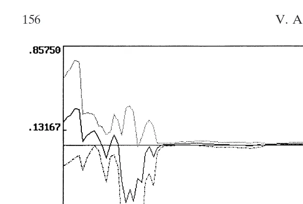
o
Twhereldepends on the frequency of the data (see Hodrick and Prescott, 1980). In Figure 3, we plot the difference betweengand the filtered series, gp, which measures temporary deviations in Italy’s government spending ratio.
The final issue is how one should allow for other influences on the real interest rate in addition to those of temporary government spending. Unlike Barro (1987), this is slightly less critical in our case, as our real interest and temporary spending variables both appear to be integrated of the same order [they are both I(0)], so that we do not face the problem of nonstationary residuals. However, there is still a potential problem of misspecification bias due to the problem of omitted influences on real interest rates. We tackle this issue in two ways. First, by allowing for an autore-gressive element (lags of the dependent variable) in equation 2,
13We also experimented with more sophisticated expectations-formation mechanisms
Figure 3. Temporary deviations ing.
so that it becomes a more conventional autoregressive distributed lag (ADL) model. Second, as in practice it is quite difficult to identify ARMA models, we try to account for unexplained influ-ences by building a structural time series model for RR with (g2
gp) as an additional explanatory variable.
The advantage of structural time series models is that they provide a more natural way of decomposing a series into its level, trend, and cyclical components than ARIMA models. Their ad-vantage over ARIMA models lie in the fact that it is simpler to identify the correct specification of structural models, and that simple specifications of structural time series models (i.e., models with a small number of estimated parameters) can be shown to have quite complex ARIMA processes as their reduced form (see Harvey, 1989). A further advantage in our context is that, although our real interest series seems I(0) when tested over the whole sample, across different policy regimes the interest rate might display local trends.
The basic structural time series model that we estimate has the general form:
bt5 bt211 zt
where the model for the interest rate, in addition to the fiscal policy explanatory variable, contains several elements. First a level component,m, which can be stochastic, and which can also have a stochastic trend term,b. The additional terms arec, which is a stochastic cycle, whose evolution is specified in Equation 4. In the cyclical element,ris the damping factor, andlcis the frequency measured in radians. This type of full structural time series model has a reduced form that is an ARIMA(2,2,4) process. Because, in our case, the real interest rate seems to be stationary, displaying a trough14 around World War II, we should find that a constant level term with no trend would be a better approximation of the behavior ofRR. If the model collapses to a cycle plus trend model with a stationary cycle, then it has a reduced form that is equal to an ARMA(2,2) process.
The structural time series model is estimated using maximum likelihood (ML), over different sample periods, to check whether the effect of temporary government spending is significant. This enables us to check whether the results from the simple ADL regression model are robust to the specification used, given the problem of misspecification bias.
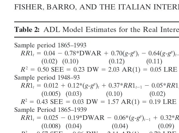
The results from the estimation of the ADL model for real interest rates are reported in Table 2. As the real interest rate behaves very erratically in the World War years due to the sudden jump in inflation, we have included, where this was significant, a step dummy for the World War years (DWAR). The AR(m) statistic is the LM test for serial correlation. The test statistics have to be interpreted with care, however, as the residuals fail both the normality test and the ARCH test when the war years are included. This is not surprising, given the behavior of the real interest rate during these years. For this reason, we also ran the same regressions over subsamples that excluded the war years. We also report the long-run impact of the temporary increase in government spending (LRE) when the equation contains distrib-uted lags or an autoregressive term. For each LRE, we also report the corresponding asymptotic standard error.
14To take account of the anomalous behavior of the real interest rate in the World War
Table 2: ADL Model Estimates for the Real Interest Rate
Sample period 1865–1993
RR1t50.0420.78*DWAR10.70(g-gp)t20.64(g-gp)t21
(0.02) (0.10) (0.12) (0.11)
R250.50 SEE50.23 DW52.03 AR(1)50.05 LRE50.06 (0.12)
Sample period 1948–93
RR1t50.01210.12*(g-gp)t10.37*RR1t2120.05*RR1t24
(0.005) (0.03) (0.10) (0.02)
R250.43 SEE50.03 DW51.57 AR(1)50.19 LRE50.18 (0.05)
Sample Period 1865–1939
RR1t50.02520.19*DWAR20.06*(g-gp)t2110.32*RR1t21
(0.008) (0.04) (0.04) (0.09)
R250.57 SEE50.06 DW52.11 AR(1)50.79 LRE5 20.09 (0.05)
Sample period 1865–1993
RR2t50.01610.010*(g-gp)t20.07*(g-gp)t2210.35*RR2t2110.19*RR2t24
(0.006) (0.02) (0.02) (0.08) (0.08)
R250.27 SEE50.05 DW52.01 AR(1)50.10 LRE50.07 (0.05)
Sample Period 1865–1939
RR2t50.00310.002*(g-gp)t11.23*RR2t2120.29*RR2t22
(0.006) (0.018) (0.112) (0.111)
R250.94 SEE50.004 DW51.94 AR(1)50.44 LRE50.03 (0.04)
Note: Standard errors reported in parentheses.
The full-sample results reported in Table 2 are poor. Over the full sample, the fiscal effect onRR1 andRR2 is insignificant (and wrongly signed forRR1). The main problem seems to be the pre-World War II data. Estimating the model over the period up to 1939 yields results that are contradictory to the neoclassical model, with an insignificant coefficient on (g 2 gp). But there is strong support for the neoclassical model in the post-World War II years. The total effect of the fiscal variable is significantly positive for the years 1948–93.15
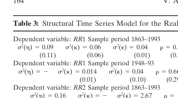
To provide a further check on the ADL model results, we estimated a structural time series model forRR1 andRR2 to see whether this might help to reconcile some of our contradictory results in Table 2.
We estimated the structural time series model over the same three sample periods. The estimated hyperparameters of the model (the parameters that govern the stochastic movements of the state variables) and the structural parameters are reported in
15We start our post-World War II sample in 1948, as the postwar inflation stabilization
Table 3: Structural Time Series Model for the Real Interest Rate
Dependent variable:RR1 Sample period 1863–1993
s2(h)50.09 s2(k)50.06 s2(e)50.04 r 50.85 l
c50.74 g 50.41
(0.11) (0.06) (0.01) (0.12) (0.12) (0.13)
Dependent variable:RR1 Sample period 1948–93
s2(h)5 2 s2(k)50.014 s2(e)50.04 r 50.66 l
c50.000 g 50.08
(0.01) (0.10) (0.29) (0.243) (0.04)
Dependent variable:RR2 Sample period 1863–1993
s2(h)50.16 s2(k)5 2 s2(e)52.67 r 5 2 l
c5 2 g 50.09
(0.07) (0.37) (0.03)
Dependent variable:RR1 Sample period 1863–1939
s2(h)5 2 s2(k)50.04 s2(e)50.001 r 50.51 l
c50.56 g 50.01
(0.03) (0.002) (0.20) (0.32) (0.06)
Dependent variable:RR2 Sample period 1863–1939
s2(h)5 2 s2(k)50.14 s2(e)50.001 r 50.97 l
c50.08 g 50.004
(0.02) (0.020) (0.02) (0.06) (0.003)
Note: Standard errors reported in parentheses.
Table 3. Note that, with the exception of the full sample estimates (1863–1993) a stochastic level is not necessary [i.e.,s2(h)], given the stationary nature of bothRR1 andRR2 over the subsamples. Similarly, a stochastic trend is not required for any of the models, and hence, estimates fors2(z) are not reported.
The structural time series model yields clearer results for the full sample. For both theRR1 andRR2 models the fiscal variable is significant, in contrast to the ADL model. Under the RR1 definition, even once a stochastic cycle is fitted to the data, the variable is still significant, which suggests that it is not picking up extraneous factors. For the 1948–93 subsample, the structural model essentially confirms the results obtained using the standard ADL model, which support the neoclassical model. For the pre-World War II period, the fiscal variable is not significant, but we do not obtain an anomalous negative estimated coefficient.
been recognized by refining the construction of the permanent component of g; (iii) the simple neoclassical model needs to be modified to explain the behavior of interest rates before 1939. For instance, some account should be taken of the effect of the threat of war on assets and hence on real interest rates. These issues could be investigated in further work.
We next turn to the possible role of debt in explaining real interest rates. There seems to be some indication that our models in Table 3 tend to underpredict the real interest rate from the 1980s onwards.
4B. Debt Accumulation and Real Interest Rates
The standard Ricardian neoclassical approach to fiscal policy suggests that debt accumulation should not influence the real interest rate (see Barro, 1987, 1989). Italy has experienced a major debt accumulation since the 1970s, and hence, provides us with an ideal context in which to test this proposition. The ratio has tended to be high throughout the historical period, but has risen sharply in the post-World War II period. We estimate our models over this latter period.
We reestimate both the ADL and structural time series models for the three sample periods, with debt as an additional explana-tory variable. Thus, the estimated equations become, for the ADL and structural time series models:
RRt5c1
o
wheredis the debt-to-GNP ratio, and we also experimented with lags of the fiscal variables in Equation 5b to find the best fit.
Table 4: The Effect of Debt on Real Interest Rates
ADL model
Sample period 1948–93
RR1t5 20.00110.08*(g-gp)t10.34*RR1t2120.06*RR1t2410.04*dt21
(0.008) (0.03) (0.10) (0.02) (0.016)
R250.47 SEE50.039 DW51.83 AR(1)50.52
LRE(g)50.11 (0.04) LRE(d)50.06 (0.02)
Structural time series model
Dependent variable:RR1 Sample period 1948–93
s2(h)5 2 s2(k)50.02 s2(e)50.04 r 50.62 l
c50.00 g050.12
(0.01) (0.01) (0.28) (0.25) (0.04)
b05 20.33 b150.39
(0.13) (0.14)
rates are unlikely to fall much without some effort to reduce the debt ratio. They tend to validate alternative theories of fiscal policies that stress the impact of the stock of public debt on interest rates (see Blanchard, 1985).
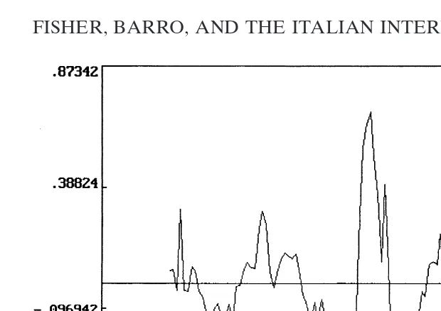
Finally, further investigation of the ADL regression in Table 4 using rolling regression methods showed that the debt variable gains significance around 1980, which corresponds to the point at which monetary policy began to be less accommodating. This is shown in Figure 4, which plots the estimated coefficient and stan-dard error bands on the dt21 regressor using a 15-observation window rolling regression. There might, therefore, be some role for the method of financing of deficits and the refinancing of debt stocks in the determination of real interest rates. The evidence might also suggest that the effect of the debt stock on real interest rates only becomes detectable at some threshold value.
5. CONCLUSIONS
In this paper we have examined some of the factors underlying the determination of nominal and real interest rates in Italy over a long historical period. There are two main conclusions from our study.
Figure 4. Estimated coefficient and standard error bands ondt21.
effect was totally absent. Nevertheless, taking the 1948–90 period as a whole, cointegration methods suggest that a unit coefficient restriction on the inflation variable cannot be rejected, validating the Fisher hypothesis.16Overall, this might suggest that inflationary expectations only adjust following sustained changes in the local trend of inflation, and that expectations do not adjust in response to short-run movements in inflation that are predictable. Barsky and DeLong (1991) provide an attractive explanation for this phenomenon, which might be attributable to uncertainty in the underlying economic structure.
Second, there seems to be evidence contrary to the pure neoclas-sical model of fiscal policy in post-World War II Italy. Although there is evidence that deviations of the government spending ratio from trend have a positive impact on real interest rates, particu-larly post-World War II, the increasing debt ratio also seems to be exerting a positive influence on real interest rates, along the lines suggested in Blanchard (1985).
16All this seems to confirm Schwartz’s statement that “. . . There (now) is less
REFERENCES
Ahmed, S. (1986) Temporary and permanent government spending in an open economy:
Some evidence for the United Kingdom.Journal of Monetary Economics17, 197–
224.
Aschauer, D.A. (1985) Fiscal policy and aggregate demand.American Economic Review
75, 117–127.
Banerjee, A., Dolado, J.J., Hendry, D.F., and Smith, G.W. (1993)Cointegration, Error
Correction and the Econometric Analysis of Stationary Data. Oxford: Oxford Univer-sity Press.
Barro, R. (1987) Government spending, interest rates, prices and budget deficits in the
United Kingdom, 1701–1918.Journal of Monetary Economics18, 221–247.
Barro, R. (1989) The neoclassical approach to fiscal policy. InModern Business Cycle
Theory(R. Barro, Ed.). Cambridge: Harvard University Press.
Barsky, R. (1987) The Fisher effect and the forecastability and persistence of inflation.
Journal of Monetary Economics19, 3–24.
Barsky, R.B., and DeLong, J.B. (1991) Forecasting pre-World War I inflation: the Fisher
effect and the gold standard.The Quarterly Journal of Economics106, 815–836.
Benjamin, D.K., and Kochin, L.A. (1984) War, prices and interest rates: a martial solution
to Gibson’s paradox. InA Retrospective on the Classical Gold Standard1821–1931
(M. Bordo and A.J. Schwartz, Eds.). Chicago: University of Chicago Press.
Blanchard, O.J. (1985) Debt, deficits and finite horizons.Journal of Political Economy93,
223–247.
Boudoukh, J., and Richardson, M. (1993) Stock returns and inflation: A long-horizon
perspective.American Economic Review83, 1346–1355.
Engle, R.F., an Granger, C.W.J. (1987) Cointegration and error-correction: Representation,
estimation and testing.Econometrica55, 251–276.
Evans (1987) Do budget deficits raise nominal interest rates? Evidence from six industrial
countries.Journal of Monetary Economics20, 281–300.
Fisher, I. (1930)The Theory of Interest. New York: Macmillan.
Friedman, M., and Schwartz, A.J. (1982)Monetary Trends in the United States and the
United Kingdom. Chicago: Chicago University Press.
Harvey, A.C. (1989)Forecasting, Structural Time Series Models and the Kalman Filter.
Cambridge: Cambridge University Press.
Hodrick, R.J., and Prescott, E.C. (1980) Postwar US business cycles: An empirical investiga-tion. Carnegie-Mellon University, Discussion Paper No. 451.
Humphrey, T.M. (1993) The early history of the real/nominal interest rate relationship. In Money, Banking and Inflation: Essays in the History of Monetary Thought. Aldershot: Edward Elgar.
Johansen, S. (1991) Statistical analysis of cointegration vectors.Journal of Economic
Dynamics and Control12, 231–254.
MacDonald, R., and Murphy, P.D. (1989) Testing for the long-run relationships between
nominal interest rates and inflation using cointegration techniques.Applied
Eco-nomics21, 439–447.
Mankiw, N.G. (1987) Government purchases and real interest rates.Journal of Political
Economy95, 407–419.
Muscatelli, V.A., and Hurn, A.S. (1994) Cointegration and dynamic time series models. In Surveys in Econometrics (D. George et al., Eds.). Oxford: Blackwells. Muscatelli, V.A., and Spinelli, F. (1996) Gibson’s Paradox and policy regimes: A
compari-son of the experience of the US, UK and Italy.Scottish Journal of Political Economy
Perron, P. (1989) The great crash, the oil price shock and the unit root hypothesis. Econo-metrica57, 1361–1401.
Pesaran, H. (1987) The Limits to Rational Expectations. Oxford: Blackwells.
Phillips, P.C.B., and Loretan, M. (1992) Estimating long-run economic equilibria.Review
of Economic Studies58, 407–436.
Rose, A. (1988) Is the real interest rate stable?The Journal of Finance43, 1095–1112.
Schwartz, A.J. (1987) A century of British market interest rates 1874–1975. InMoney in
Historical Perspective. Chicago: University of Chicago Press.
Spinelli, F., and Fratianni, M. (1991)Storia Monetaria d’Italia. Milano: Arnoldo Mondadori.
Summers, L.H. (1983) The non-adjustment of nominal interest rates: A study of the Fisher
effect. In Macroeconomics, Prices and Quantities(J. Tobin, Ed.). Symposium in
memory of A. Okun. Washington, DC: The Brookings Institution.
Summers, L.H. (1986) Estimating the long-run relationship between interest rates and
inflation.Journal of Monetary Economics18, 77–86.
Wallace, M.S., and Warner, J.T. (1993) The Fisher effect and the term structure of interest