arXiv:1711.06674v1 [math-ph] 17 Nov 2017
COMPARING NETS AND FACTORIZATION ALGEBRAS OF OBSERVABLES: THE FREE SCALAR FIELD
OWEN GWILLIAM, KASIA REJZNER
Abstract. In this paper we compare two mathematical frameworks that make perturbative quantum
field theory rigorous: the perturbative algebraic quantum field theory (pAQFT) and the factorization algebras framework developed by Costello and Gwilliam. To make the comparison as explicit as possible, we focus here on the example of the free scalar field. The main claim is that both approaches are equivalent if one assumes the time-slice axiom. The key technical ingredient is to use time-ordered products as an intermediate step between a net of associative algebras and a factorisation algebra.
Contents
1. A preview of the key ideas 2
1.1. Classical theories 2
1.2. Quantization 3
2. Nets versus factorization algebras 4
2.1. Notations 4
2.2. Overview of the pAQFT setting 5
2.3. Overview of factorization algebras 7
2.4. A variant definition: locally covariant field theories 10
3. Comparing the definitions 12
3.1. Models of the free scalar field 12
3.2. The comparison results 13
3.3. Key ingredients of the argument 14
3.4. The time-slice axiom and the algebra structures 17
4. Constructing the CG model for the free scalar field 19
4.1. The classical model 19
4.2. The quantum model 22
5. Constructing the pAQFT model for the free scalar field 22
5.1. A dg version of pAQFT 23
5.2. Constructing the dg models 24
6. Proof of comparison theorems 27
6.1. The classical case 27
6.2. The quantum case 28
6.3. The associative structures 28
6.4. Shifted vs. unshifted Poisson structures 29
7. Interpretation of the results 29
7.1. The main lesson 30
7.2. Yet another perspective 31
7.3. A summary by way of a dictionary 31
8. Outlook and next steps 32
8.1. Interacting scalar field theories 32
8.2. Lifting Wick rotation to the algebraic level 33
8.3. Gauge theories 34
Acknowledgments 34
Date: November 20, 2017.
References 34
Recently there have appeared two, rather elaborate formalisms for constructing the observables of a quantum field theory via a combination of the Batalin-Vilkovisky framework with renormalization methods. One [FR12b] works on Lorentzian manifolds and weaves together (a modest modification of) algebraic quantum field theory (AQFT) with the Epstein-Glaser machinery for renormalization. The other [CG17a, CG17b] works with elliptic complexes (i.e., “with Euclidean theories”) and constructs factorization algebras using renormalization machinery developed in [?]. To practitioners of either for-malism, the parallels are obvious, in motivation and techniques and goals. It is thus compelling (and hopefully eventually useful!) to provide a systematic comparison of these formalisms, with hopes that a basic dictionary will lead in time to effortless translation.
The primary goal in this paper is to examine in detail the case of free scalar field theory, where renor-malization plays no role and we can focus on comparing the local-to-global descriptions of observables. In other words, in the context of this free theory, we show how to relate the key structural features of AQFT and factorization algebras. In the future we hope to compare interacting field theories, which demands an examination of renormalization’s role and deepens the comparison by touching on more technical features.
A secondary goal of this paper is to facilitate communication between communities, by providing a succinct treatment of this key example in each formalism. We expect that interesting results—and questions!—can be translated back and forth.
One consequence of this effort at comparison is that it spurred a modest enhancement of each formal-ism. On the pAQFT side, we introduce a differential graded (dg) version of the usual axioms for the net of algebras. Prior work fits nicely into this definition, and in the future we hope to examine its utility in gauge theories. On the CG side, we show that the free field construction applies to Lorentzian manifolds as well as Euclidean manifolds. (The case of interacting theories in the CG formalism does not port over so simply, as it exploits features of elliptic complexes in its renormalization machinery.)
As an overview of the paper, we begin by raising key questions about how the formalisms agree and differ. To sharpen these questions, we give precise descriptions of the outputs generated by each formalism, namely the kinds of structure possessed by observables. On the FR side, one has a net of algebras; on the CG side, a factorization algebra of cochain complexes. With these definitions in hand, we can state our main results precisely. As a brief, imprecise gloss, our main result is that the FR and CG constructions agree where they overlap: if one restricts the CG factorization algebra of observables to the opens on which the FR net is defined (and takes the zeroth cohomology), then the factorization algebra and net determine the same functor to vector spaces. We also explain how one can recover as well the algebraic structures on the nets (Poisson for the classical theory, associative for the quantum) from the constructions. Next, we turn to carefully describing theconstructionsin each formalism, so that we can prove the comparison results. We recall in detail how each formalism constructs the observables for the free scalar field, producing on the one hand, a net of algebras on a globally hyperbolic Lorentzian manifold, and on the other, a factorization algebra. With the constructions in hand, the proof of the comparison results is straightforward. Finally, we draw some lessons from the comparison and point out natural directions of future inquiry.
1. A preview of the key ideas
Before delving into the constructions, we discuss field theory from a very high altitude, ignoring all but the broadest features, and explain how each formalism approaches observables. With this knowledge in hand, it is possible to raise natural questions about how the formalisms differ. The rest of the paper can be seen as an attempt to answer these questions.
1.1. Classical theories. A classical field theory is specified, loosely speaking, by (1) a smooth manifoldM (the “spacetime”),
(2) a smooth fiber bundle over the manifold π : F → M whose smooth sections Γ(M, π) are the “fields,”
(3) and a system of partial differential equations on the fields (the “equations of motion” or “Euler-Lagrange equations”) that are variational in nature.
We will write the equations asP(φ) = 0whereφis a field andP denotes the equations of motion. (There are many variations and refinements on this loose description, of course, but most theories fit into this framework.)
In this paper, the focus is on the free scalar field theory. Here the manifold M is equipped with a metricg, and an important difference is that the FR formalism requires gto have Lorentzian signature while the CG formalism requiresg to be Riemannian. The fiber bundle is the trivial rank one vector bundleF =M×R→M so that the fields are simplyC∞(M,R), the smooth functions on M. We will discuss issues of functional analysis later, but note that we equip C∞(M,R) with its natural Frechét topology and use the standard notationE(M)for it.
The differential equations can be concisely given, since they play such a central role throughout physics and mathematics:
△gφ+m2φ= 0,
where △g denotes the Laplace-Beltrami operator for the metric (sometimes called a d’Alembertian for the Lorentzian case) andm∈R+ called the “mass.”
A crucial feature of field theory is that it is local on the manifoldM. Note, to start, that the fieldsE
form a sheaf that assigns to an open setU, the set
E(U) = Γ(U, πU :π−1(U)→U)
of smooth sections of the bundle overU. That is,Edefines a contravariant functorE:Open(M)op→Set from the poset categoryOpen(M)of open sets inM to the category of sets. As global smooth sections are patched together from local smooth sections,Eforms a sheaf of sets onM. (It also forms a sheaf of vector spaces and of topological vector space.)
Consider nowSol(M), the set of solutions to the equations of motion, i.e., the configurations (or fields) that are allowed by the physical system described by the classical field theory. (We ignore here, since we’re speaking vaguely, whether we should consider solutions that are not smooth, such as distributional solutions and whether we ought to impose boundary conditions.) Since differential equations are, by definition, local onM, solutions to the equations of motion actually form a sheaf onM . That is, if we write
Sol(U) ={φ∈E(U) : P(φ) = 0}
for sections on U that satisfy the equations of motion, then Sol also defines a contravariant functor Sol : Open(M)op
→ Set. As global solutions are patched together from local solutions, Sol forms a sheaf of sets onM.
Any measurement of the system should then be some function ofSol(M), the set of global solutions. In other words, the algebra of functionsO(Sol(M))constitutes an idealized description of all potential measuring devices for the system. (An important issue later in the text will be what kind of functions we allow, but we postpone that challenge for now, simply remarking that solutions often form a kind of “manifold,” possibly singular and infinite-dimensional, so thatOis not merely set-theoretic.) Even better,
we obtain a covariant functor O(Sol(−)) : Open(M)→ CAlg to the category CAlg of commutative algebras. As Solis a sheaf, O(Sol(−))should be a cosheaf, meaning that it satisfies a gluing axiom so that the global observables are assembled from the local observables.
Nothing about this general story depends on the signature of the metric, and each formalism gives a detailed construction of a cosheaf of commutative algebras for a classical field theory (although some technical choices differ, e.g., with respect to functional analysis). It is withquantum field theories that the formalisms diverge.
1.2. Quantization. Loosely speaking, the formalisms describe the observables of a quantum field theory as follows.
• The CG formalism provides a functorObsq :Open(M)→Ch, which assigns a cochain complex (or differential graded (dg) vector space) of observables to each open set. This cochain complex is a deformation of a commutative dg algebraObscl, whereH0(Obscl(U)) =O(Sol(U)).
• The FR formalism provides a functorA:C(M)→Alg∗, which assigns a unital∗-algebra to each
“causally convex” open set (so thatC(M)is a special subcategory ofOpen(M)depending on the global hyperbolic structure ofM). The algebraA(U)is, in practice, a deformation quantization of the Poisson algebraO(Sol(U)).
In brief, both formalisms deform the classical observables, but they deform it in different ways. In Section
2we give precise descriptions of both formalisms. Two questions jump out:
(1) Why does the FR formalism (and AQFT more generally) restrict to a special class of opens but the CG formalism does not? And what should the FR formalism assign to a general open? (2) Why does the FR formalism (and AQFT more generally) assign a∗-algebra but the CG formalism
assigns only a vector space? And can the CG approach recover the algebra structure as well? Both questions admit relatively simple answers, but those answers require discussion of the context (e.g., the differences between elliptic and hyperbolic PDE) and of the BV framework for field theory. We will organize our treatment of the free scalar field toward addressing these questions.
2. Nets versus factorization algebras
This section sets the table for this paper. We begin with some background notation (which is mostly self-explanatory, so we suggest the reader only refer to it if puzzled) before reviewing quickly the key definitions about nets and factorization algebras. We made an effort to make the definitions accessible to those from the complementary community.
2.1. Notations.
2.1.1. Functional analysis. We will follow the conventions that began with Schwartz for various function spaces:
• E(M)=. C∞(M),
• E′(M)for the topological dual (i.e., the space of continuous linearR-valued functions on a given topological space), which consists of compactly supported distributions,
• D(M)=. C∞
c (M), and
• D′(M)for the topological dual (i.e., the space of continuous linearR-valued functions on a given topological space), which consists of non-compactly supported distributions.
We indicate the complexification of a real vector spaceV by a superscriptVC
.
As we work throughout with manifolds equipped with a metric, we use the associated volume form of (M, g)to identify smooth functions with densities. Hence we have preferred inclusions E(M)֒→D′(M) andD(M)֒→E′(M).
Remark 1. We note that these conventions differ from those in [?], whereE(M)is used to denote the smooth sections of a vector bundleE→M,Ec(M)the compactly supported smooth sections,E(M)the distributional sections, andEc(M)the compactly supported distributional sections. As we stick to scalar fields (i.e., sections of the trivial rank one bundle) throughout this paper, we hope there is no confusion. 2.1.2. Categories. Myriad categories will appear throughout this work, and so we introduce some of the key ones, as well as establish notations for generating new ones. Categories will be indicated in bold.
We start with a central player. Let Nucdenote the category of nuclear, topological locally convex
vector spaces, which is a subcategory of the category of topological locally convex spaces TVec. It is
equipped with a natural symmetric monoidal structure via the completed projective tensor product⊗b
(although we could equally well say ‘injective’ as the spaces are nuclear).
Remark 2. Given the spaces appearing in our construction, it is often worthwhile to work instead with convenient vector spaces [KM97], but we will not discuss that machinery here, pointing the interested reader to [CG17a,Rej16].
If we wish to discuss the category of unital associative algebras of such vector spaces, we write
Alg(Nuc). Here the morphisms are continuous linear maps that are also algebra morphims. Similarly,
we writeCAlg(Nuc)for unital commutative algebras inNucandPAlg(Nuc)for unital Poisson algebras therein. We will typically want∗structures (i.e., an involution compatible with the multiplication), and we useAlg∗(Nuc), CAlg∗(Nuc), andPAlg∗(Nuc), respectively.
More generally, for C a category with symmetric monoidal structure ⊗, we write Alg(C⊗)for the unital algebra objects in that category. Often we will write simply Alg(C), if there is no potential
confusion about which symmetric monoidal structure we mean.
In a similar manner, ifC is an additive category, we writeCh(C)to denote the category of cochain complexes and cochain maps inC. ThusCh(Nuc)denotes the category of cochain complexes inNuc
(which, unfortunately, is not a particular nice place to do homological algebra). This category admits a symmetric monoidal structure by the usual formula: the degreek component of the tensor product of two cochain complexes is
(A•
⊗B•)k= M i+j=k
Aib ⊗Bj.
Hence we writeAlg(Ch(Nuc))for the category of algebra objects, also known as dg algebras.
Remark 3. This categoryCh(Nuc)admits a natural notion of weak equivalence: a cochain map is a weak equivalence if it induces an isomorphism on cohomology. Thus it is a relative category and presents an(∞,1)-category, although we will not need such notions here.
There is another important variant to bear in mind. In the oroginal axiomatic framework of Haag and Kastler, the notion of subsystems is encoded in the injectivity requirement for algebra morphisms. We use the superscript “inj”, if we want to impose this condition on morphisms, for a given category. HenceAlg∗(Nuc)injconsists of the category whose objects are nuclear, topological locally convex unital ∗-algebras but whose morphisms areinjectivecontinuous algebra morphisms.
2.1.3. Dealing with~. In perturbative field theory, one works with~as a formal variable. In our situation, since we restrict to free fields, this is overkill: one can actually set ~ = 1 throughout, and all the constructions are well-defined. But ~ serves as a helpful mnemonic for what we are deforming and as preparation for the interacting case.
We thus introduce categories involving ~ that emphasize its algebraic role here and minimize any topological issues. One ought to take more care in the interacting case.
LetNuc~ denote the following category. For our constructions we only need vector spaces that are
free as modules overC[[~]], so we identify the objects inNuc~ with the class of objects inNuc. Given
V ∈Nuc, we thus useV[[~]] to denote the corresponding object inNuc~. (The reader shouldthink of
this space asQn≥0~nV.) As we want a morphism to encode an~-linear map of such free modules, it should be determined by where the ~0V component of V[[~]] would go. Hence, we define the space of morphisms to be
HomNuc~(V[[~]], W[[~]]) =
Y
n≥0
~nHomNuc(V, W),
where the ~n is just a formal bookkeeping device. Composition is by precisely the rule one would use for ~-linear maps. For instance, given f = (~nfn) ∈ HomNuc~(V[[~]], W[[~]]) and g = (~ngn) ∈ HomNuc~(W[[~]], X[[~]]), the compositeg◦f has
(g◦f)0=g0◦f0,
(g◦f)1=g1◦f0+g0◦f1, ..
. since informally we want
(X n≥0
~ngn)◦(X
m≥0
~mfm) =X
p≥0
X
m+n=p
~pgn◦fm.
We equip this category with a symmetric monoidal structure borrowed fromNuc:
V[[~]]⊗b~W[[~]] = (V⊗bW)[[~]].
Note that it agrees with the completed tensor product over C[[~]], in the same sense that composition of morphisms does.
The category Alg(Nuc~) then consists of algebra objects in that symmetric monoidal category, Ch(Nuc~)denotes cochain complexes therein, andAlg(Ch(Nuc~))denotes dg algebras therein.
2.2. Overview of the pAQFT setting. The framework of AQFT formalizes rigorously the core ideas of Lorentzian field theory, building on the lessons of rigorous quantum mechanics, but the standard calculational toolkit for interacting QFT does not fit into the framework. Perturbative AQFT is a natural modification of the framework within which one often can realize a version of the usual calculations, while preserving the structural insights of AQFT.
2.2.1. LetM= (M, g)be an n-dimensional spacetime, i.e., a smoothn-dimensional manifold with the metricg of signature(+,−, . . . ,−). We assumeMto be oriented, time-oriented and globally hyperbolic
(i.e. it admits foliation with Cauchy hypersurfaces). To make this concept clear, let us recall a few important definitions in Lorentzian geometry.
Definition 1. Let γ : R ⊃I → M be a smooth curve in M, for I an interval in R and let γ˙ be the vector tangent to the curve. We say that γis
• timelike, ifg( ˙γ,γ)˙ >0,
• spacelike, ifg( ˙γ,γ)˙ <0,
• lightlike(or null), if g( ˙γ,γ) = 0,˙ • causal, ifg( ˙γ,γ)˙ ≥0.
The classification of curves defined above is thecausal structure ofM.
Definition 2. A setO⊂Miscausally convexif for any causal curve γ: [a, b]→Mwhose endpoints γ(a), γ(b)lie inO, then every interior point γ(t), for t∈[a, b], also lies inOfor every t∈[a, b].
With these definitions in hand, we can define the category of open subsets on which we specify algebras of observables.
Definition 3. LetCaus(M)be the collection of relatively compact, connected, contractible, causally con-vex subsetsO⊂M. Note that the inclusion relation⊂is a partial order onCaus(M), so(Caus(M),⊂) is a poset (and hence a category).
2.2.2. To formulate a classical theory, we start with making precise what we mean by the model for the space of classical fields.
Definition 4. A classical field theory model on a spacetime M is a functor P : Caus(M) →
PAlg∗(Nuc)inj that obeys Einstein causality, i.e.: for O1,O
2 ∈Caus(M)that are spacelike to each other, we have
⌊P(O1),P(O2)⌋O={0},
where⌊., .⌋O is the Poisson bracket in anyP(O)for anOthat contains both O1 andO2.
Note how this definition formalizes the sketch of classical field theory in Section1: we have a category of opens — here,Caus(M)— and a functor to a category of Poisson algebras, since the observables of a classical system should form such a Poisson algebra. The underlying commutative algebra is then referred to as the space of classical fields. More precisely, letc:PAlg∗(Nuc)→CAlg(Nuc)denote the forgetful functor. Later on we will also need the forgetful functors to vector spaces,v:PAlg∗(Nuc~)→Nuc~
andv:Alg∗(Nuc~)→Nuc~.
Definition 5. The space of classical fields is defined asc◦P.
It is useful to introduce a further axiom that articulates more precisely how the dynamics of a classical theory should behave. Here, a time orientation plays an important role.
Definition 6. Given the global timelike vector field u(the time orientation) onM, a causal curveγ is calledfuture-directedif g(u,γ)˙ >0all alongγ. It is past-directedif g(u,γ)˙ <0.
Definition 7. A causal curve is future inextendible if there is no p ∈M such that for every open neighborhood U ofp, there existst′ such that γ(t)
∈U for allt > t′.
Definition 8. A Cauchy hypersurface inMis a smooth subspace of Msuch that every inextendible causal curve intersects it exactly once.
Remark 4. The significance of Cauchy hypersurfaces lies in the fact that one can use them to formulate the initial value problem for partial differential equations, and for normally hyperbolic equations this problem has a unique solution.
With this notion in hand, we have a language for enforcing equations of motion at an algebraic level. Definition 9. A model is said to beon-shell if in addition it satisfies thetime-slice axiom: for any
N ∈ Caus(M) a neighborhood of a Cauchy surface in the region O ∈ Caus(M), then P(N) ∼= P(O). Otherwise the model is called off-shell.
Remark 5. Note that being on-shell codifies the idea that the set of solutions is specified by the initial value problem on a Cauchy hypersurface.
2.2.3. We now turn to the quantum setting.
Definition 10. A QFT model on a spacetime M is a functor A : Caus(M) → Alg∗(Nuc~)inj that
satisfiesEinstein causality(Spacelike-separated observables commute). That is, forO1,O2∈Caus(M) that are spacelike to each other, we have
[A(O1),A(O2)]O={0},
Definition 11. A QFT model is said to be on-shell if in addition it satisfies the time-slice axiom
(where one simply replacesP by Ain the definition above). Otherwise, it isoff-shell.
Often a quantum model arises from a classical one by means of quantization. In order to formalize this, we need some notation. Given a functorF, letF[[~]]denote the functor sendingOtoF(O)⊗bC[[~]].
Definition 12. A quantum modelAis said to be a quantization of a classical modelP, if: (1) v◦A∼=v◦P[[~]],
(2) c◦P∼=A/(~). (3) The brackets −i
~[., .]O coincides with{., .}O modulo ~.
Later, it will be important to have a generalization of definitions that assigns a dg algebra to each
O∈Caus(M). Recall that a dg algebra is aZ-graded vector spaceA=
L
nAn equipped with
• a grading-preserving associative multiplication⋆so thata ⋆ b∈Am+n ifa∈Amandb∈An, an • a differential d : A→ A that increases degree by one, satisfies d2 = 0, and is a derivation, so
that
d(a ⋆ b) = da ⋆ b+ (−1)|a|a ⋆db for homogeneous elementsa, b∈A.
This generalization appears naturally when one adopts the BV framework for field theory, as it uses homological algebra in a serious way. We introduce these dg models in Section5.1.
2.3. Overview of factorization algebras. In their work on chiral conformal field theory, Beilinson and Drinfeld introduced factorization algebras in an algebro-geometric setting. These definitions also encompass important objects in geometric representation theory, playing a key role in the geometric Langlands program. Subsequently, Francis, Gaitsgory, and Lurie identified natural analogous definitions in the setting of manifolds, which provide novel approaches in, e.g., homotopical algebra and configuration spaces. Below we describe a version of factorization algebras, developed in [CG17a], that is well-suited to field theory.
As this brief history indicates, factorization algebras do not attempt to axiomatize the observables of a field theory. Instead, they include examples from outside physics, such as from topology and representation theory, and permit the transport of intuitions and ideas among these fields. We will explain below further structure on a factorization algebra that makes it behave like the observables of a field theory in the Batalin-Vilkovisky formalism.
2.3.1. The core definitions. Let M be a smooth manifold. Let Open(M) denote the poset category whose objects are opens inM and where a morphism is an inclusion. A factorization algebra will be a functor fromOpen(M)to a symmetric monoidal categoryC⊗equipped with further data and satisfying further conditions. We will explain this extra information in stages. (Note that almost all the definitions below apply to an arbitrary topological space, or even site with an initial object, and not just smooth manifolds.)
Definition 13. A prefactorization algebra F on M with values in a symmetric monoidal category
C⊗ consists of the following data:
• for each open U ⊂M, an objectF(U)∈C,
• for each finite collection of pairwise disjoint opens U1, . . . , Un and an open V containing every Ui, a morphism
F({Ui};V) :F(U1)⊗ · · · ⊗F(Un)→F(V),
and satisfying the following conditions:
• composition is associative, so that the triangle
N
i
N
jF(Tij)
N
iF(Ui)
F(V)
commutes for any collection{Ui}, as above, contained inV and for any collections{Tij}j where for eachi, the opens{Tij}j are pairwise disjoint and each contained in Ui,
• the morphisms F({Ui};V)are equivariant under permutation of labels, so that the triangle
F(U1)⊗ · · · ⊗F(Un) F(Uσ(1))⊗ · · · ⊗F(Uσ(n))
F(V) ≃
commutes for anyσ∈Sn.
Note that if one restricts to collections that are singletons (i.e., someU ⊂V), then one obtains simply a precosheaf F : Open(M) →C. By working with collections, we are specifying a way to “multiply”
elements living on disjoint opens to obtain an element on a bigger open. In other words, the topology ofM determines the algebraic structure. (One can use the language of colored operads to formalize this interpretation, but we refer the reader to [CG17a] for a discussion of that perspective. Moreover, one can loosen the conditions to be homotopy-coherent rather than on-the-nose.)
A factorization algebra is a prefactorization algebra for which the value on bigger opens is determined by the values on smaller opens, just as a sheaf is a presheaf that is local-to-global in nature. A key difference here is that we need to be able to reconstruct the “multiplication maps” from the local data, and so we need to modify our notion of cover accordingly.
Definition 14. AWeiss cover {Ui}{i∈I} of an open subset U ⊂M is a collection of opens Ui⊂U such that for any finite set of pointsS ={x1, . . . , xn} ⊂U, there is somei∈I such thatS ⊂Ui.
Remark 6. Note that a Weiss cover is also a cover, simply by considering singletons. Typically, however, an ordinary cover is not a Weiss cover. Consider, for instance, the case where U = V ⊔V′, with V, V′ disjoint opens. Then
{V, V′
} is an ordinary cover by not a Weiss cover, since neither V nor V′ contains any two element set {x, x′
} with x ∈ V and x′
∈ V′. Nonetheless, Weiss covers are easy to construct. For instance, cover an n-manifold M by taking the collection of all open subsets that are locally homeomorphic to a finite union of copies ofRn.
This notion of cover determines a Grothendieck topology onM; concretely, this means it determines a notion of cover for each open of M that behaves nicely with respect to intersection of opens and refinements of covers. In particular, we can talk about (co)sheaves relative to this Weiss topology onM.
Definition 15. Afactorization algebraFis a prefactorization algebra onM such that the underlying precosheaf is a cosheaf with respect to the Weiss topology. That is, for any openU and any Weiss cover {Ui}{i∈I} ofU, the diagram
`
i,jF(Ui∩Uj)
`
iF(Ui) F(U)
is a coequalizer.
Typically, our target category C is vector spaces of some kind (such as topological vector spaces),
in which case the coproducts`denote direct sums and the coequalizer simply means thatF(U)is the cokernel of the difference of the maps for the inclusionsUi∩Uj ⊂Ui andUi∩Uj ⊂Uj. Note that we have implicitly assumed that Cpossesses enough colimits, and we will assume that henceforward.
Remark 7. In fact, our target category is usually cochain complexes of vector spaces, and we want to view cochain complexes as (weakly) equivalent if they are quasi-isomorphic. Hence, we want to work in an ∞-categorical setting. In such a setting, the cosheaf condition becomes higher categorical too: we replace the diagram above by a full simplicial diagram over the Čech nerve of the cover and we require
F(U)to be the homotopy colimit over this simplicial diagram. For exposition of these issues, see [CG17a]. In practice, another condition often holds, and it’s certainly natural from the perspective of field theory.
Definition 16. A factorization algebraFismultiplicativeif the map
F(V)⊗F(V′)→F(V ⊔V′)
is an isomorphism for every pair of disjoint opensV, V′.
In brief, ifFis a multiplicative factorization algebra, one can reconstructFif one knows how it behaves
on a collection of small opens. For instance, supposeM is a Riemannian manifold and one knowsFon
how to reconstruct from a Weiss basis.) Our examples are often multiplicative, or at least satisfy the weaker condition that the map is a dense inclusion.
Note that there is a category of prefactorization algebrasPFA(M,C⊗) where each object is a pref-actorization algebra on M and where a morphism η : F → G consists of a collection of morphisms
inC,
{η(U) :F(U)→G(U)}U∈Open(M)
such that all the multiplication maps intertwine. The factorization algebras form a full subcate-goryFA(M,C⊗).
2.3.2. Relationship with field theory. By now, the reader may have noticed that there has been no discus-sion of fields or Poisson algebras or so on. Indeed, the definitions here are more general and less involved than for the AQFT setting because they aim to apply outside the context of field theory (e.g., there are interesting examples of factorization algebras arising from geometric representation theory and algebraic topology) and because there is no causality structure to track. By contrast, AQFT aims to formalize precisely the structure possessed by observables of a field theory on Lorentzian manifolds, and hence must take into account both causality and other characterizing features of field theories (e.g., Poisson structures at the classical level).
Let us briefly indicate how to articulate observables of field theory in this setting, suppressing impor-tant issues of homological algebra and functional analysis, which are discussed below in the context of the free scalar field and in [CG17a,CG17b] in a broader context. The necessary extra ingredient is that on each open U, the objectF(U)has an algebraic structure.
Definition 17. Given prefactorization algebrasF,GonM, letF⊗Gdenote the prefactorization algebra with
(F⊗G)(U) =F(U)⊗G(U) and the obvious tensor product of structure maps.
In other words, the category of prefactorization algebrasPFA(M,C⊗)is itself symmetric monoidal. In many cases the full subcategory FA(M,C⊗) is closed under this symmetric monoidal product. In particular, if the tensor product⊗inCpreserves colimits separately in each variable (or at least geometric
realizations), thenF⊗Gis a factorization algebra whenF,Gare.
Thus, if C is some category of vector spaces, one can talk about, e.g., a commutative algebra in PFA(M,C⊗). That meansFis equipped with a map of prefactorization algebras·:F⊗F→Fsatisfying
all the conditions of a commutative algebra. Similarly, one can talk about Poisson or∗-algebras. It is equivalent to say thatFis inCAlg(PFA(M,C⊗))or to say it is a prefactorization algebra with values in CAlg(C⊗), the category of commutative algebras in C⊗. This equivalence does not apply,
however, to factorization algebras, due to the local-to-global condition: a colimit of commutative algebras does not typically agree with the underlying colimit of vector spaces. For instance, in the category of ordinary commutative algebrasCAlg(Vec⊗), the coproduct isA⊗B, but in the category of vector spaces
Vec, it is the direct sum A⊕B. (This issue is very general: for an operadO, the categoryO-alg(C⊗) of O-algebras has a forgetful functor to C that always preserves limits but rarely colimits.) Thus, a
commutative algebra in factorization algebrasF∈CAlg(PFA(M,C⊗))assigns a commutative algebra to every open U and a commutative algebra map to every inclusion of disjoint opensU1, . . . , Un ⊂V, but it satisfies the coequalizer condition inC, not inCAlg(C⊗).
This terminology lets us swiftly articulate a deformation-theoretic view of the Batalin-Vilkovisky framework.
Definition 18. A classical field theory model is a 1-shifted Poisson (aka P0) algebra P in factor-ization algebrasFA(M,Ch(Nuc)). That is, to each openU ⊂M, the cochain complexP(U)is equipped with a commutative product· and a degree 1 Poisson bracket{−,−}; moreover, each structure map is a map of shifted Poisson algebras.
In parallel, we have the following.
Definition 19. Aquantum field theory modelis a Beilinson-Drinfeld (BD) algebraAin factorization algebrasFA(M,Ch(Nuc~)). That is, to each openU ⊂M, the cochain complexA(U)is flat overC[[~]]
and equipped with
• an~-linear commutative product·,
• a differential such that
d(a·b) = d(a)·b+ (−1)aa·d(b) +~{a, b}.
Moreover, each structure map is a map of BD algebras.
Note that for any BD algebraA, there is adequantization Acl=A⊗C[[~]]C[[~]]/(~)
that is automatically a 1-shifted Poisson algebra. Hence every quantum field theory model dequantizes to a classical field theory model. Given a classical field theory modelP, one can ask if it quantizes, i.e.,
if there exists a quantum field theoryAwhose dequantization is P.
Remark 8. The condition on the differential is an abstract version of a property possessed by the divergence operator for a volume form on a finite-dimensional manifold. Thus, the differential of a BD algebra behaves like a “divergence operator,” as explained in Chapter 2 of [CG17a], and hence encodes (some of) the kind of information that a path integral would.
2.4. A variant definition: locally covariant field theories. Above, we have worked on a fixed manifold, but most field theories are well-defined on some large class of manifolds. For instance, the free scalar field theory makes sense on any manifold equipped with a metric of some kind. Similarly, (classical) pure Yang-Mills theory makes sense on any 4-manifold equipped with a conformal class of metric and a principalG-bundle. One can thus replaceOpen(M)by a more sophisticated category whose objects are “manifolds with some structure” and whose maps are “structure-preserving embeddings.” (In the scalar field case, think of manifolds-with-metric and isometric embeddings.) In a field theory, the fields restrict along embeddings and the equations of motion are local (but depend on the local structure), so that solutions to the equationsSolforms a contravariant functor out of this category. Likewise, one can generalize the models of classical or quantum field theory to this kind of setting, as we now do.
Remark 9. This discussion is not necessary for what happens elsewhere in the paper, so the reader primarily interested in our comparison results should feel free to skip ahead.
2.4.1. The Lorentzian case. We begin by replacing the fixed spacetime Mby a coherent system of all
such spacetimes.
Definition 20. Let Locn be the category where an object is a connected, (time-)oriented globally hy-perbolic spacetime of dimension n and where a morphism χ : M→ N is an isometric embedding that preserves orientations and causal structure. The latter means that for any causal curve γ: [a, b]→N, if γ(a), γ(b)∈χ(M), then for all t∈]a, b[, we haveγ(t)∈χ(M). (That is, χ cannot create new causal links.)
We can extendLocn to a symmetric monoidal categoryLoc⊗n by allowing for objects that are disjoint unions of objects inLocn. The relevant symmetric monoidal structure is the disjoint union⊔. Note that
a morphism inLoc⊗n must send disjoint components to spacelike-separated regions.
We are now ready to define what is meant by a locally covariant field theory in our setting.
Note that isotony is implicit in the requirement that morphisms inAlg∗(Nuc)inj are injective. It is likewise implicit in the following definitions.
Definition 21. A locally covariant classical field theory model of dimension n is a functor P :
Locn →PAlg∗(Nuc)inj such that theEinstein causality holds: given two isometric embeddingsχ1 :
M1→Mandχ1:M1→Mwhose imagesχ1(M1)andχ2(M2)are spacelike-separated, the subalgebras
Pχ1(P(M1))⊂P(M)⊃Pχ2(P(M2))
Poisson-commute, i.e., we have
⌊Pχ1(a1),Pχ2(a2)⌋={0}, for any a1∈P(M1)anda2∈P(M2).
Definition 22. A locally covariant quantum field theory model of dimension n is a functor A:Locn→Alg∗(Nuc~)injsuch that Einstein causality holds:
Given two isometric embeddings χ1:M1→Mandχ1:M1→Mwhose imagesχ1(M1) andχ2(M2)are spacelike-separated, the subalgebras
commute, i.e., we have
[Aχ1(a1),Aχ2(a2)] ={0},
for anya1∈A(M1)anda2∈A(M2).
Definition 23. A model P (A) is called on-shellif it satisfies in addition the time-slice axiom: If χ : M → N contains a neighborhood of a Cauchy surface Σ ⊂ N, then the map Pχ : P(M)→ P(N) (Aχ:A(M)→A(N)) is an isomorphism.
Remark 10. The categoryAlg∗(Nuc)injhas a natural symmetric monoidal structure via the completed tensor product ⊗b. Then Einstein causality can be rephrased as the condition that A is a symmetric monoidal functor fromLoc⊗n toAlg∗(Nuc)inj,⊗b, as discussed in [BFIR14].
2.4.2. The factorization algebra version. Let us begin with the simplest version.
Definition 24. Let Embn denote the category whose objects are smooth n-manifolds and whose mor-phisms are open embeddings. It possesses a symmetric monoidal structure under disjoint union.
Then we introduce the following variant of the notion of a prefactorization algebra. Below, we will explain the appropriate local-to-global axiom.
Definition 25. Aprefactorization algebra onn-manifoldswith values in a symmetric monoidal category
C⊗ is a symmetric monoidal functor fromEmbn toC⊗.
This kind of construction works very generally. For instance, if we want to focus on Riemannian manifolds, we could work in the following setting.
Definition 26. Let Riemn denote the category where an object is Riemannian n-manifold(M, g)and a morphism is open isometric embedding. It possesses a symmetric monoidal structure under disjoint union.
Definition 27. A prefactorization algebra on Riemannian n-manifolds with values in a symmetric monoidal categoryC⊗ is a symmetric monoidal functor fromRiemn toC⊗.
Remark 11. In these definitions, the morphisms in Riemn form a set, but one can also consider an enrichment so that the morphisms form a space, perhaps a topological space or even some kind of infinite-dimensional manifold. This kind of modification can be quite useful. For instance, this would allow to view isometries (i.e., isometric isomorphisms) as a Lie group, rather than as a discrete group.
In general, let G denote some kind of local structure for n-manifolds, such as a Riemannian metric
or complex structure or orientation. In other words, G is a sheaf on Embn. A Gstructure on an n-manifold M is then a section G ∈ G(M). There is a category EmbG whose objects are n-manifolds
withGstructure(M, GM)and whose morphisms areGstructure-preserving embeddings, i.e., embeddings
f : M ֒→N such that f∗GN = GM. This category is fibered overEmbG. One can then talk about prefactorization algebras onG-manifolds.
We now turn to the local-to-global axiom in this context.
Definition 28. A Weiss cover of a G-manifold M is a collection of G-embeddings {φi : Ui → M}i∈I such that for any finite set of pointsx1, . . . , xn ∈M, there is somei such that{x1, . . . , xn} ⊂φi(Ui).
With this definition in hand, we can formulate the natural generalization of our earlier definition.
Definition 29. A factorization algebra onG-manifolds is a symmetric monoidal functor F:EmbG→ C⊗ that is a cosheaf in the Weiss topology.
One can mimic the definitions of models for field theories in this setting.
Definition 30. AG-covariant classical field theoryis a 1-shifted (akaP0) algebraPin factorization algebras FA(EmbG,Ch(Nuc)).
Definition 31. A G-covariant quantum field theory is a Beilinson-Drinfeld (BD) algebra A in factorization algebras FA(EmbG,Ch(Nuc~)).
3. Comparing the definitions
Now that we have the key definitions in hand, we can restate the questions (1.2) more sharply. (1) In the CG formalism a model for a field theory defines a functor on the poset Open(M) of
all open subsets. By contrast, the FR formalism a model defines a functor on the subcategory
Caus(M). Why this restriction? How should one extend an FR model to a functor on the larger
category of all opens? Is it a factorization algebra?
(2) In the FR formalism, a model assigns a Poisson algebra (or∗-algebra) to each open inCaus(M),
whereas in the CG formalism, a model assigns a shifted Poisson algebra (or BD algebra) to every open. Are these rather different kinds of algebraic structures related?
We will address these questions in the specific example of free scalar field theory. In the conclusion, we draw some lessons and hints about the case of interacting theories and non-scalar theories.
3.1. Models of the free scalar field. We now turn to stating our main result, which is a comparison of the FR and CG procedures. First, we need to state what each formalism accomplishes with the free scalar field. In the following sections, we spell out in detail how to construct the models asserted and prove the propositions.
We remark that these statements are likely hard to understand at this point; thepointis just that we get models in both the FR and CG senses.
Proposition 1. Let M = (M, g) be a d-dimensional, oriented, time-oriented, and globally hyperbolic spacetime with the metricg of signature(+,−, . . . ,−). For each massm, there is a classical field theory model Pfor the free particle of mass mon Msuch that
• The space of fields F(O)is the space generated (as a commutative algebra) by continuous linear functionals on distributional solutions ofφ+m2φ= 0 onO;
• the commutative product · is the obvious pointwise product of the space of functionals on the solution space ofO;
• the Poisson bracket is the Peierls bracket ⌊., .⌋.
There is a quantum field theory model A for the free particle of mass m on Msuch that for each O∈ Caus(M), the associative C[[~]]-algebra A(O)is generated topologically by continuous linear functionals on distributional solutions toφ+m2φ= 0 and the product⋆ satisfies the relation
[F, G]⋆ =i~⌊F, G⌋ for linear functionalsF, G.
Remark 12. Note that allowing for distributional solutions enforces a restriction on the dual, so that F is generated by functionals of the formφ7→Rφf, wheref is a compactly supported test density on M, modulo the ideal generated by functionals of the formφ7→R φ(+m2φ)f.
Analogously, the CG approach to free theories applies to Lorentzian manifolds, as we show below, and we obtain the following.
Proposition 2. Let M = (M, g) be a d-dimensional, oriented, time-oriented, and globally hyperbolic spacetime with the metricg of signature(+,−, . . . ,−). For each massm, there is a classical field theory model P for the free particle of mass m, i.e., a P0 algebra in factorization algebras P on M where for each open U ⊂M, the commutative dg algebraP(U)is generated topologically by the cochain complex
D(U)[1]−−−−→+m2 D(U).
It is equipped with the degree 1 Poisson bracket by using the Leibniz rule to extend the pairing on gener-ators
⌊f−1, f0⌋=
Z
U
f−1f0dvolg,
withf−1in degree -1 andf0 in degree 0. There is a quantum field theory modelAfor the free particle of mass m, i.e., a BD algebra in factorization algebras onM whereA(U)is the BD quantization ofP(U) whose differential isdP+~△, where the BV Laplacian △is determined by the fact that△ vanishes on
constants and on the linear generators.
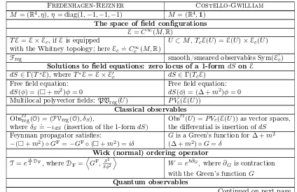
To summarize, we have the following collection of models.
FR CG
classical P P
quantum A A
We remark that these propositions might seem distinct on the surface, since the CG result involves cochain complexes while the FR result does not. This distinction disappears when one examines the actual constructions: both use a BV framework, and hence the FR construction actually builds a cochain-level functor as well. We formalize a dg version of pAQFT in Section 5.1 below, which makes the comparison even more obvious.
3.2. The comparison results. With these models in hand, a clean comparison result can be stated. Before making the formal statement, we first explain it loosely.
The basic idea is that we can restrict the factorization algebras to Caus(M), since every
causally-convex open is manifestly an open subset and hence there is an inclusion functorCaus(M)֒→Open(M). The restrictionsP|Caus(M)and A|Caus(M)can be further simplified by taking cohomology on eachO∈
Caus(M): we define functors
H∗(P)|Caus(M)(O) =H∗(P(O))
and
H∗(A)|Caus(M)(O) =H∗(A(O)).
This cohomology is always concentrated in degree zero. We then want to compare the functors H0(P/A)
|Caus(M) to the corresponding FR functors. The targets of these functors, however, are different. For instance,Ptakes values in 1-shifted Poisson algebras
and hence so does H0P (although the bracket must then be trivial for degree reason). By contrast, P takes values in Poisson∗-algebras. Hence we apply forgetful functors to lad in the same target category. We now state our comparison result for the classical level.
Theorem 1(Comparison of classical models). There is a natural transformation ιcl:c◦P|Caus(M)⇒c◦P
of functors to commutative dg algebras CAlg(Ch(Nuc)), and this natural transformation is a quasi-isomorphism (up to a topological completion). Thus, there is a natural quasi-isomorphism
H0(ιcl) :c◦H0(P)|Caus(M) ∼ = ⇒c◦P of functors into commutative algebras CAlg(Nuc).
This identification is not surprising, as both approaches end up looking at (a class of) functions on solutions to the equations of motion.
We can extend to the quantum level, but here we need the forgetful functorv:Alg∗(Nuc~)→Nuc~,
sinceH0Aisa priorijust a vector space.
Theorem 2(Comparison of quantum models). There is a natural transformation ιq :A
|Caus(M)⇒v◦A
of functors to Ch(Nuc~), and this natural transformation is a quasi-isomorphism (up to a topological
completion). Thus, there is a natural isomorphism
H0(ιq) :H0(A)|Caus(M) ∼ = ⇒v◦A.
Modulo ~, this isomorphism agrees with the isomorphism of classical models.
In fact, on eachO∈Caus(M), the mapιq is an isomorphism of cochain complexes
α∂GD :v(P(O)[[~]])
∼ =
−→v(A(O))
determined by the analytic structure of the equations of motion. Under this identification, the factoriza-tion structure ofAagrees with the time-ordered version of the product ⋆GC on A.
In other words, the factorization algebraAknows information equivalent to the QFT modelA.
Con-versely, one can recover fromA, the precosheaf structure ofArestricted toCaus(M). (This assertion is
true when one uses the cochain-level refinement of A, as we will see below when reviewing the explicit FR construction.)
What is more important is that there is a natural way to identify the algebra structures on either side. We will show that one can read off the FR deformation quantizationAfrom the CG factorization algebraAand conversely. But this second part of the quantum comparison theorem is likely cryptic at
the moment, as it involves the notationα∂GD and terminology “time-ordered products” that we have not
yet introduced. These, however, are the key to understanding how the two approaches to QFT relate, so we now discuss them in some detail.
3.3. Key ingredients of the argument. In this section we recall the relevant background about quantum field theories, notably the notions appearing in the theorems above. We explain, in particular, how the associative algebra structure appears inA, why it is important to the physics, and how it relates to constructions in the CG formalism.
3.3.1. Time-ordered products and why they are important. The free quantum theory is fully characterized by the net A, but in order to deal with interactions, we need one more structure, namely the time-ordered product. Constructing time-time-ordered products of free fields is an intermediate step towards building interacting fields. The idea is analogous to using the interacting picture in quantum mechanics. Namely, we would like to apply the Dyson formula to define the time evolution operator as a time-ordered exponential:
Here :−: denotes the normal-ordering,T denotes time-ordering, H0 denotes the free Hamiltonian, and HI denotes the the interacting Hamiltonian, which is the operator-valued function of spacetime
HI(x) =eiH0x0:HI(0,x):e−iH0x0.
Heuristically, one could use the unitary map defined above to obtain interacting fields as (1) φI(x) =U(x0, s)−1φ(x)U(x0, s) =U(t, s)−1U(t, x0)φ(x)U(x0, s), fors < x0< t.
To put this approach on a rigorous footing, the framework of pAQFT replaces the Dyson series by theformal S-matrix:
n is a linear map from appropriate domain in C∞(E,C)⊗n to C∞(E,C)[[~]], and the above expression is to be understood as a power series in the coupling constant λ with coefficients in Laurent series in ~. Constructiong S is then reduced to
constructionTn’s, which in turn is done using the Epstein-Glaser renormalization [EG73].
In [FR12a] it was shown that the maps Tn arise from a commutative, associative product·T defined
on a certain domain contained inC∞(E,C)[[~]]. Here, to avoid problems related to renormalization, we will consider·T on a yet smaller domain, namelyFreg[[~]]. (See Definition35for its description.)
More abstractly, we introduce the following notion.
Definition 32. Given the classical free off-shell theory P and its quantization A, the time-ordered productis realized as a triple (AT, ξ,T)consisting of a functor
AT:Caus(M)→CAlg∗(Nuc~),
where mT/m⋆ is the multiplication with respect to the time-ordered/star product and the relation “≺”
means “not later than,” i.e., there exists a Cauchy surface in Othat separates ψ1(O1)and ψ2(O2). (In the first case,ψ1(O1)is in the future of this surface, and in the second case, it is in the past.) This triple collectively provides an equivalence between the time-ordered product ·T of AT and the classical product·
whereF, G∈AT(O).
This definition intertwines the product on classical and quantum observables in a nontrivial way, and as mentioned in Theorem2, it is the key to relating the algebraic structures on Aand A. Hence our
goal is to construct this time-ordered product on free fields and show how it appears in the comparison map ιq. We explain that in the next few subsections, which are thus somewhat technical. The main ingredient is various propagators, or Green’s functions, for the equation of motion.1
3.3.2. Propagators. We introduce the four key propagators, which are linearly related.
Symbol Meaning
GA advanced propagator GR retarded propagator GC=. GR
−GA causal propagator GD=. 12 GR+GA Dirac propagator
Note that the causal propagator isnota Green’s function but rather a bisolution, so (+m2)GC= 0
whereas for the others
(+m2)GA/R/D=δ∆,
whereδ∆denotes the delta function of the diagonalM ֒→M×M. The advanced (respectively, retarded) propagatorGA(x, y)has the property that it vanishes when the first pointxis in the “past” (respectively, “future”) ofy.
The causal propagator GC is related to another important type of a bi-solution of P, namely the Hadamard function.
Definition 33. A Hadamard functionG+ for a normally hyperbolic operator P is a distribution in
D′(M2)satisfying:
(1) G+ is a distributional bi-solution for P. (2) 2 ImG+=GC
(3) G+ fulfills the microlocal spectrum condition: its wavefront set2is
WF(G+) ={(x, k;x,−k′)∈T M˙ 2|(x, k)∼(x′, k′), k∈(V+)x},
where (x, k)∼(x′, k′) means that there exists a null geodesic connectingx andx′ and k′ is the parallel transport of k along this geodesic, T˙ denotes the tangent bundle with the zero section removed and(V+)x is the closure of the cone of positive, future-pointing vectors inT∗
xM. (4) G+is of positive type, i.e. G+, f⊗f¯≥0, for all non-zerof ∈D(M)⊗C. The bracket denotes
the dual pairing between distributions and test functions. Note that anyG+ can be written as
G+= i 2G
C+H ,
whereH is a real, symmetric distributional bi-solution forP. TheFeynman propagator associated with this Hadamard functionG+ is then defined as
GF=iGD+H .
For notational convenience, we refer to both bi-solutions and Green’s functions aspropagators. We extend our table of propagators with
Symbol Meaning
G+=. i 2G
C+H Hadamard function GF=. iGD+H Feynman propagator forG+
1
Indeed, this project began when we realized we were using the same tricks with propagators.
2Thewavefront setof a distributionu∈D′(Rn)is a subset ofT˙∗Rn(the co-tangent bundle minus the zero section)
characterizing singular points and singular directions of u (i.e.,directions in the cotangent space in which the Fourier transform does not decay rapidly). More precisely, the complement ofWF(u)inT˙∗Rn
is the set of points(x, k)∈T˙∗Rn
for which there exists a “bump function”f∈D(Rn
)withf(x) = 1and an open conic neighborhoodCofk, with
sup k∈C
(1 +|k|)N|fd·u(k)|<∞ ∀N∈N0.
This notion easily generalizes to open subsets ofRn and to manifolds [Hör03]. Note that if aW F(u) =∅, then uis a
smooth function.
The propagators listed above can be used to define (1) new products on the observables and
(2) automorphisms of the (underlying vector spaces of) observables. In the following sections we will explain these constructions in detail.
3.3.3. Smooth maps on between locally convex vector spaces. In this work, we model observables asC[[~ ]]-valued functions on the space of solutions to some linear differential equations (elliptic or hyperbolic). On various stages of the comparison between the CG and FR approaches, we also consider functions between arbitrary locally convex topological vector spaces. For such functions one can introduce the notion ofsmoothness, which we are going to refer to later on. We start by introducing smooth functions on E(M). For future convenience, we state here the general definition of a functional derivative of a function between two Hausdorff locally convex spaces.
Definition 34. LetU be an open subset of a Hausdorff locally convex spaceX and letF be a map from U to a Hausdorff locally convex space Y. Then F has a derivative at x∈ U in the direction of v∈X if the following limit
D
F(1)(x), vE:= lim t→0
F(x+tv)−F(x)
t ,
exists. The function F is said to have a Gâteaux differential at x if F(1)(x), v exists for every v ∈X. F is C1 or Bastiani differentiable [Bas64, Mic38] on U if F has a Gâteaux differential at every x∈U and the mapF(1):U ×X →Y defined by (x, v)7→F(1)(x), v is continuous on U×E.
This definition applies in particular to functions from E(M) to C. Iterating it n times we define Cn-functionals of E(M). If a functional is Cn for all n
∈ N, we call it (Bastiani) smooth and write F ∈C∞(E(M),C). Detailed properties of such functionals have been investigated in [BDLGR17].
Localization properties of smooth functionals on E(M)are characterized by the notion of spacetime support:
(2) suppF =. {x∈M| ∀O∋xopen,∃φ, ψ∈Es.t. ψ⊂OandF(φ+ψ)6=F(φ)} This definition is equivalent to (see [BDLGR17, Lemma 3.3])
(3) suppF =. [
φ∈E(M)
suppF(1)(φ).
Among all smooth functionals, a special role is played by the regular ones. Regularity properties of a smooth functional are formulated in terms of the wavefront (WF) sets of its derivatives, since F(n)(φ)
∈E′(Mn,C)(see [BDLGR17, section 3.4] for the proof).
Definition 35. A functionalF is regularif WF(F(n)(φ))is empty for allφ
∈E,n∈N, i.e., F(n)(φ)
∈DC
(Mn).
We denote the space of regular functionals by Freg.
3.3.4. Exponential products. A propagator G is an element of D′(M2) and as such, so can be viewed as a bi-vector field on E. To see this, note that since E is a vector space, we have TE = E×E, so
(TE)⊗2 =E×E⊗2, where we define the completion of the tensor product by E⊗2 =. D′(M2). Hence (TE)⊗2is a trivial bundle with the space of section beingC∞(E(M),D′(M2))andGis a constant section of this bundle.
Let F be a smooth functional on E with smooth derivatives, i.e. F ∈ Freg. We use the suggestive notation∂G to denote the differential operator constructed fromGas follows:
∂GF =. ιG(F(2)),
whereιG(F(2))(φ) =G, F(2)(φ)and the pairing is induced by the duality betweenD′(M2)andD(M2). The propagatorGcan also be viewed as a section of(TE(M))⊠2 (here⊠denotes the exterior tensor product, so the completed space of sections is C∞(E
×E,D′(M2)) and we write ∂G to denote the differential operator:
˜
∂G(F1⊗F2)=. ιG(dF1⊠dF2),
Definition 36. Given a constant-coefficient second-order differential operator ∂G, we define an˜ expo-nential productby
F1⋆GF2=m◦e~∂˜G(F1⊗F2),
wherem denotes the usual commutative multiplication, i.e. pullback by the diagonal mapφ7→φ⊗φ.
Direct computation shows that⋆G is associative. As we will see later, the product structure ofA(O) comes from⋆GC.
One can also define automorphisms (of underlying vector spaces) by
αG(F) =e~2∂GF.
(When G2−G1 is symmetric, αG2−G1 determines an isomorphism of algebras from the⋆G1 product to
the⋆G2 product.) Such a map allows us also to define the time-ordered product by
(4) F1·TF2=αiGD(α−1
iGD(F1)·α
−1 iGD(F2)).
This definition has the crucial property that
F1·TF2=T(F1⋆GCF2)
when the observablesF1 andF2 have disjoint supports andT denotes the time-ordering
T(F1⋆GCF2) =
F1⋆GCF2 if F2≺F1
F2⋆GCF1 if F1≺F2,
Note here the connection with the Dyson formula: ·T agrees with the usual time-order prescription for
⋆GC and extends it to regular functionals with overlapping supports.
Those familiar with the CG approach, notably Section 4.6 of [CG17a], will recognize that this definition is precisely the factorization product onA.
3.4. The time-slice axiom and the algebra structures. A dissatisfying aspect of the comparison results is that they involve forgetful functors: it seems like we ignore the crucial Poisson, respectively associative, algebra structures, although the constructions (e.g., with propagators) certainly involved them. As discussed, these algebraic structures play a crucial role in physics and hence appear in the axioms of AQFT, but they are not built into the CG construction. It is natural to ask how to resolve this tension.
We provide two perspectives that we feel clarify substantially this issue, one rooted in a key maneuver of the FR work and another using results in higher algebra in conjunction with the CG perspective. Both depend on a prominent and useful feature of these examples: they satisfy the time-slice axiom. That is, if Σ is a Cauchy hypersurface for nested opens O ⊂ O′ in Caus(M), then A(O) → A(O′) is an isomorphism. The factorization algebra satisfies a cochain-level analog of this axiom: the map
A(O)→A(O′)is a quasi-isomorphism.
The time-slice property suggests formulating a version ofAandAliving just on a Cauchy hypersurface
itself. We will state a natural comparison result before explaining the idea why one should exist from the CG perspective.
3.4.1. The result on comparison of algebraic structures. We now turn to formulating a precise framework for describing how the algebraic structures intertwine.
LetΣbe a Cauchy hypersurface of M, and letOpenr(Σ)denote the poset of open subsets ofΣthat are relatively compact.
Fix a small tubular neighborhood ofΣ⊂Σe insideMthat is causally convex.
Definition 37. Let A|Σ : Openr(Σ) → Alg(Nuc) denote the functor that assigns toU, the algebra A(OU), whereOU is the maximal open inCaus(M), contained in Σ, for which˜ U is a Cauchy hypersur-face.
Alternatively, we could set
A|Σ(U) = lim
O⊃U is Cauchy
A(O),
taking the limit over opensU ∈Caus(M)for whichU is a Cauchy hypersurface. It was shown in [Chi08] that this algebra is naturally isomorphic to the algebra obtained by quantizing the Cauchy data.
Likewise, we provide a version ofA|Σ. One could use a limit construction, but we prefer something
more concrete. For each open U ⊂ Σ, let Ue denote the maximal causally convex open in Σe whose intersection withΣisU.
Definition 38. Let A|Σ : Openr(Σ) → Ch(Nuc~) denote the functor that assigns to U, the BD
algebra A(Ue).
We thus obtain a nice comparison statement.
Theorem 3. Let Σbe a Cauchy hypersurface ofM. The functorA|Σcan be lifted to a dg algebra A|AlgΣ inFA(Σ,Ch(Nuc~)). In particular, the functorH0ιq|Σ of Theorem2lifts to a natural isomorphism
H0ιq
|AlgΣ :H0(A|Σ)Alg ∼ = ⇒A|Σ of functors to algebras.
We prove this result in Section6, after we spell out the explicit constructions of our models.
There is an obvious classical analogue to this result. The associative algebraH0(A|Σ)is naturally filtered by powers of ~, and its associated graded algebra is isomorphic to the commutative algebra H0(P|Σ)[[~]]. Hence, the commutative algebra c◦H0(P|Σ) acquires an unshifted Poisson bracket, by taking the~-component of the commutator of the associative algebra.
Corollary 1. There is a functor
H0(P|Σ)P ois:Openr(Σ)→PAlg(Nuc)
by using the Poisson bracket induced on c◦H0(P
|Σ) since it is the associated graded of H0(A
|Σ). The functorH0ιcl
|Σof Theorem 1lifts to a natural isomorphism H0ιcl|P oisΣ :H0(P|Σ)P ois
∼ = ⇒P|Σ of functors to Poisson algebras.
A version of this statement at the cochain-level, for P, would also be appealing. We now turn to
explaining a version that relies on homotopical algebra, but in Section 6.4 we use formulas to explain how the Peierls bracket follows from the BV bracket.
3.4.2. The argument via higher abstract nonsense. We wish to explain why P and A, when restricted
to a Cauchy hypersurface, obtain Poisson and associative structures, respectively. A priori they have a shifted Poisson and BD structure, however. How could this transmutation of algebraic structure occur? The key is a pair of interesting results from higher algebra that will relate certain factorization algebras to associative and Poisson algebras. We state the results before extracting the consequence relevant to us.
LetE1denote the operad of little intervals. Concretely, anE1algebraA∈AlgE1(Ch)is a homotopy-associative algebra; in particular, every E1 algebra is weakly equivalent to some dg algebra. The first result, due to Lurie [Lur17], says that there is an equivalence of∞-categories
AlgE
1(Ch)≃FA
lc
(R,Ch),
where the superscript lc means we restrict to locally constant factorization algebras: a factorization algebra F on R is locally constant if the map F(I) → F(I′) is a quasi-isomorphism for every pair of nested intervalsI ֒→I′. Lurie’s result says that a locally constant factorization algebra onRencodes a homotopy-associative algebra andvice versa.
The second result explains how to relate different kinds of shifted Poisson algebras. Let Pn denote the operad encoding(1−n)-shifted Poisson brackets, so thatP1algebras are the usual Poisson algebras (in a homotopy-coherent sense).
Theorem 4(Poisson additivity, [Saf16]). There is an equivalence of∞-categories
AlgE1(AlgP oisn(Ch))≃AlgP oisn+1(Ch).
Forn= 0, these results combine to say that a locally constant factorization algebra with a 1-shifted Poisson structure determines a homotopy-coherent version of an 0-shifted Poisson algebra. Now consider the map q : M → R by taking the leaf space with respect to the foliation by Cauchy surfaces. The pushforward factorization algebraq∗Phas a 1-shifted Poisson structure but it is also locally constant,
since the solutions to the equation of motion is a locally constant sheaf in terms of the “time” parameter R. Hence, by general principles, we know thatq∗Pdetermines a 0-shifted Poisson algebra.
In this case, the homotopy-Poisson algebra must be strict at the level of cohomology, since the coho-mologyH∗Pis concentrated in degree 0. This strict Poisson structure agrees with the Poisson structure onP, as we will see.