e
u
*Flow Fields in front of a Cylindrical Obstacle
Yulistiyanto, B.1)
Abstract: An experimental investigation, conducted in two different flows Reynolds number, was carried out to study the structure of the flow field upstream of a cylindrical obstacle. An Acoustic Doppler Velocity Profiler (ADVP) was used to obtain instantaneously the three directions of the mean velocity. Results of the experiments show the longitudinal velocities,
u
, decrease approaching the cylinder, their distribution becomes more uniform and close to the bed a reverse flow is noticeable with increasing importance. The downward velocity component is clearly shown, continuing with the return flow near the bed, forming a vortex. At positions where the vortex appears upstream from the cylinder, a large increase of the three components of the turbulence intensities is remarked. Approaching the cylinder, one observes the shear stress decreases, having the opposite direction at positions close to the cylinder. A zero value of shear stress should be at the separation point.
Keywords: cylindrical obstacle, experimental investigation, velocities distributions, vortex.
Introduction
A complex flow fields is established if flow is disturbed by an obstacle. The flow upstream will undergo a separation of the turbulent boundary layer and rolls up to form the well-known horseshoe-vortex system. This type of flow occurs in a variety of situations, such as flow around bridge piers, around buildings and structures, and at different types of junctions.
The experiments done with airflow over round and round-nosed objects have been investigated by numerous authors [1-5] and with free surface flow [6,7]. Similar experiment measurements were conducted for flow around a vertical semicircular cylinder attached to the sidewall [8] and at a wing-wall abutment installed at a rectangular channel [9]. This study investigates flow fields upstream a cylinder by using experiment data conducted in open channel.
Research Method
Measurements of velocity and turbulence upstream a cylindrical obstacle was conducted for two different flows Reynolds number (Re). For the first run namely Test 1, Re = 1.24 105 was used, while the second run namely Test 2, used Re = 0.74 105. The experiments were conducted in a 43.0 m long, 2.0 m wide and 1.0 m high tilting flume.
1 Civil and Environmental Engineering Department, Faculty of Engineering, Gadjah Mada University, Yogyakarta, Indonesia Email: [email protected]; [email protected]
Note: Discussion is expected before November, 1st 2010, and will be published in the “Civil Engineering Dimension” volume 13, number 1, March 2011.
Received 11 May 2009; revised 22 December 2009; accepted 24 March 2010.
The flume can be tilted with the bottom-slope range of -0.5% to 3.5%. A smooth-surface PVC cylinder having a diameter of D = 22.0 cm and a height of H = 0.5 m, was used to simulate the cylindrical obstacle. The ratio of the channel width to the cylinder diameter was 9.1.
The velocity and turbulence profiles at some measuring station were measured using the Acoustic Doppler Velocity Profiler (ADVP) instrument for 60 seconds using an emission frequency of 1 MHz. Data analyses were then performed to get the velocity and turbulence profiles at different height of 4.65 mm intervals. Cylindrical coordinates are used to denote the position of the measuring station in which P (r,
α, z) and Q (r, α, z) refer to one of Test 1 and of Test 2, respectively. In which r is the distance from the center of cylinder to P or Q, and α is equal to zero degree for upstream directions of an obstacle position, and z is the vertical distance from the bed. Ten measurement points were selected upstream from the cylinder, at distance varying from 12 to 44 cm, smaller intervals were adopted for those close to the cylinder.
The friction velocities are calculated at first using the energy gradient, Sf, which is equal to the bed slope
for uniform flow, Sf =So, using the following formula:
f
e ghS
u∗ = (1)
where, , g, h and Sf are the friction velocity,
acceleration of gravity, flow depth, and energy gradient, respectively. Subsequently the Weisbach-Darcy coefficient, f, is calculated using Equation 2.
(
)
2/ 8u U
where U is the flow velocity. These calculated values are summarized in Table 1. The semi-empirical equation of Colebrook and White [10] given by Equation 3, is then used to determine the uniform roughness, ks:
flow Reynolds number, respectively. The roughness Reynolds number, (ksu*e/ν), can now be calculated
(Table 1). It can be concluded that the channel bed is in the transitional regime [10].
Results of Measurements and Discussion
The measurements upstream from the cylinder for Test 1 and Test 2, α1=α2=0°, were taken at 10 to 11 different stations with the distance of the measurement from the center of the cylinder, r, in the range of 12.0 cm to 44.0 cm, or r/D of 0.5 to 2.
The tristatic ADVP-instrument performed the measurements from P (44.0, 0°, z) to P (15.0, 0°, z), and from Q (44.0, 0°, z) to Q (14.0, 0°, z), resulting in the three directions of the mean velocity profiles as well as their turbulence intensity and two components of the Reynolds stresses. Measurements at P (14.0, 0°, z) to P (12.0, 0°, z), and at Q (13.0, 0°, z) to Q (12.0, 0°, z) were also done by the tristatic ADVP-instrument system in the y-z plane, giving results of the velocity profiles in the transversal,
v
, and in the vertical,w
, directions and their turbulence intensity, v′2 and 2w′ ; as well as results
of the Reynolds stress in the transversal direction,
w
v′ ′. The value of time-averaged shear stress was calculated by averaging a large number of calculated instantaneous shear stress values obtained from measurement [12]. Results of these measurements are presented and discussed in the followings.
Velocity profiles
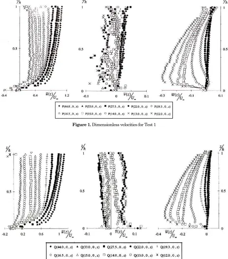
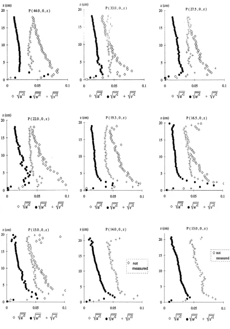
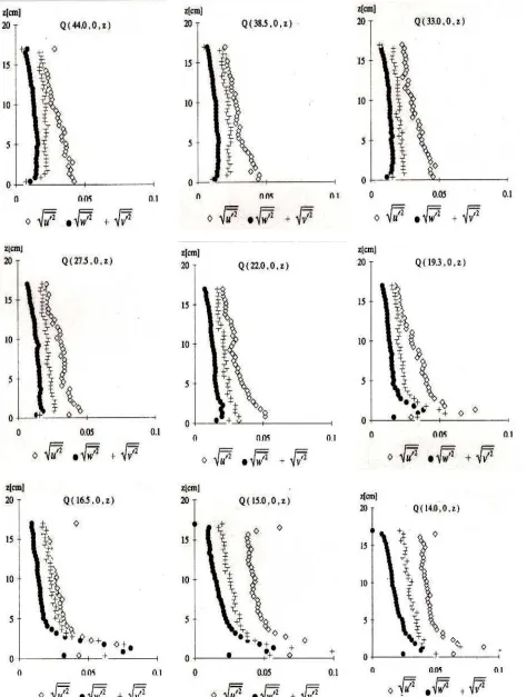
Figures 1 and 2 show the profiles of the mean velocity along the symmetry plane upstream from the cylinder adimensionalized by the approach velocity, U∞, are plotted against the relative depth,
z/h. Approaching the cylinder one observes (Figures 1 and 2) the followings: the longitudinal velocities,
,
u
decrease; their distribution becomes more uniform, and close to the bed a reverse flow is noticeable with increasing importance. Profiles of measurements far from the cylinder have the logarithmic distribution, whereas close to the cylinder, from P (15.0, 0°, z) to P (12.0, 0°, z) and fromQ (15.0, 0°, z) to Q (12.0, 0°, z), the shape of u(z)/U∞ becomes more rectangular, and the maximum velocity is already reached far away under the water surface.
The vertical (downward) velocity,
w
, distributions at measurements far from the cylinder are small. Approaching the cylinder, their values increase and have a quasi triangular shape for measurements close to the cylinder, from P (15.0, 0°, z) to P (12.0, 0°,z) and from Q (16.5, 0°, z) to Q (14.0, 0°, z). Its distributions have a zero value at the surface and a maximum value near the bed. The downward velocity component increases while the longitudinal component decreases. The maximum downward flow is about
w
= 0.3U∞ at P (12.0, 0°, z) for Test 1, andw
= 0.35U∞ at Q (12.0, 0°, z) for Test 2. These are smaller values than those presented by Ettema [10]. Ettema's measurement at 0.02-0.05D from the cylinder wall, gave a maximum value ofw
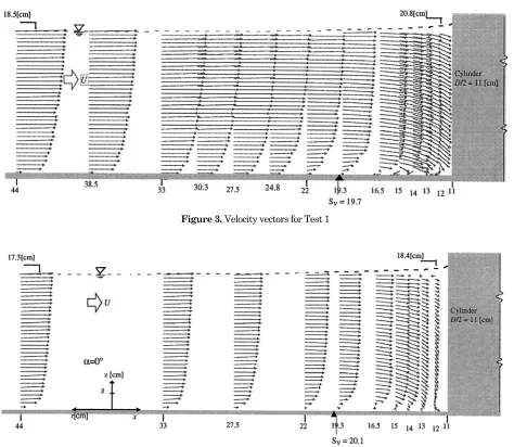
= 0.4 U∞, near the bed. The mean transversal velocity,v, is uniform over the depth and is much smaller compared to the longitudinal and the vertical ones, conclusion can be deduced to indicate the effect of the cylinder. Fig. 3 and Fig. 4 show the velocity vectors of the bidimensional velocities, ur andw
, for Test 1and Test 2, respectively. The ur, equivalent to the
negative longitudinal velocity, -u, decreases as it approaches the cylinder. The downward flow near the edge of the cylinder is clearly shown, continuing with the return flow near the bed, forming a vortex. The position of the separation point, Sv, could not be exactly defined from this velocity vector, due to the small measurement density in the radial direction. However, this position can be presumed to be between the last positive velocity and the next negative (reverse) velocity at the bed, which lies between r = 19.5 cm and r = 22.0 cm for both tests.
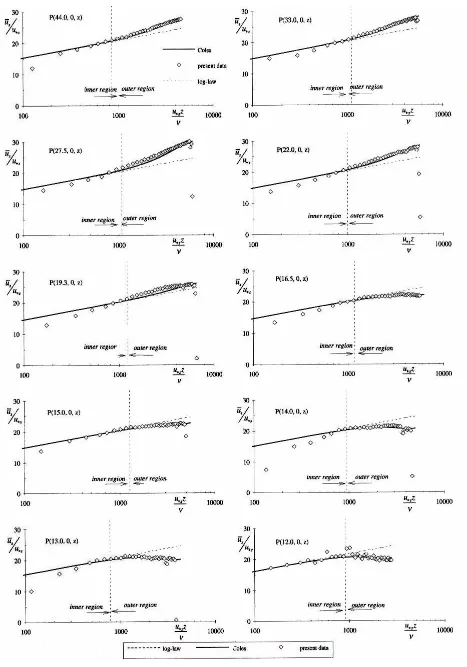
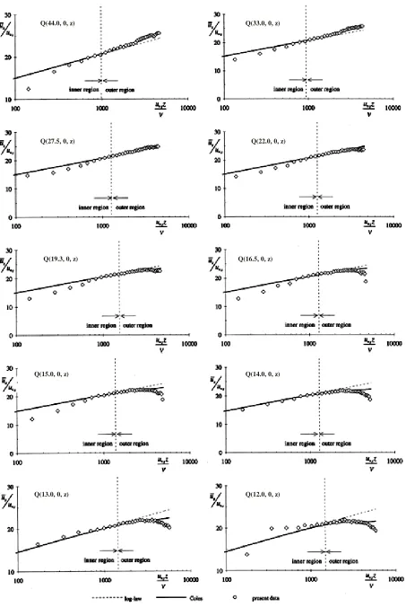
The longitudinal velocity profiles for Test 1 and Test 2, plotted as u
( )
z /u*cl against( )
u*clz /v, are presentedTable 1. Uniform flow parameter and friction velocities.
Test U
[m/s]
e
u
∗[m/s] f ks
ν
e su
k ∗
u
∗r[m/s]
cl
u
∗[m/s] r
r cl
u u u
∗ ∗ ∗ −
r r e
u u u
∗ ∗ ∗ −
1 0.67 0.034 0.0202 0.00043 14.5 0.029 0.0310 6.9% 17%
2 0.43 0.022 0.0206 0.00038 8.4 0.021 0.0207 -1.4% 4.7%
Note:
U is the flow velocity; u*r and u*clare the friction velocities found from Reynolds stress distribution and Clauser Method.
Figure 1. Dimensionless velocities for Test 1
The measured data are then evaluated using this logarithmic velocity distribution, Eq. 2. The friction velocity, u * cl can then be calculated (according to Clauser [10]), and the constant of integration, Btr, by trial and error. These values are summarized in Table 2. The numerical constant of integration, Btr, is in agreement with the ones in the literature [10].
It is shown in Figs. 5 and 6, that the profiles in the inner region coincide quite well with the log-law, Eq. 2, except for points near the bed. These unexpected points are due to a part of the measurement volumes that are under the mylar [12]. However for measurements close to the cylinder, from Q (15.0, 0°,
z) to Q ( 12.0 , 0°, z), some points near the bed fall
Figure 3. Velocity vectors for Test 1
Figure 4. velocity vectors for Test 2
Table 2. The friction velocity, constant of integration, and wake strength
Position (r, α, z)
u
* s[m/s] Btr Π
Position (r, α, z)
u
* s[m/s] Btr Π
P (44.0,0,z) 0.0260 9.949 0.60 Q (44.0,0,z) 0.0294 9.940 0.25
P (33.0,0,z) 0.0315 9.984 0.75 Q (33.0,0,z) 0.0280 9.927 0.30
P (27.5,0,z) 0.0335 9.986 1.10 Q (27.5,0,z) 0.0285 9.971 0.15
P (22.0,0,z) 0.0320 9.985 0.80 Q (22.0,0,z) 0.0285 9.971 0.10
P (19.3,0,z) 0.0365 9.982 0.30 Q (19.3,0,z) 0.0293 9.976 -0.20
P (16.5,0,z) 0.0350 9.985 -0.5 Q (16.5,0,z) 0.0298 9.978 -0.20
P (15.0,0,z) 0.0310 9.983 -0.4 Q (15.0,0,z) 0.0310 9.983 -0.30
P (14.0,0,z) 0.0280 9.968 -0.8 Q (14.0,0,z) 0.0330 9.986 -0.45
P (13.0,0,z) 0.0240 9.920 -0.9 Q (13.0,0,z) 0.0352 9.985 -0.40
Q(44.0, 0, z) Q(33.0, 0, z)
Q(27.5, 0, z) Q(22.0, 0, z)
Q(14.0, 0, z) Q(19.3, 0, z)
Q(15.0, 0, z)
Q(12.0, 0, z) Q(13.0, 0, z)
Q(16.5, 0, z)
below the logarithmic line. These maybe caused by the influence of the presence of the vortex. The velocity distribution in the outer region, z/h > 0.2, deviates from the log-law, as shown in Figs. 5 and 6. Coles [10] developed a formula for this region as follows: parameter. In Eq. 5, all values are known and the wake strength parameter, Π, can be determined; they are listed in Table 2.
The data in the outer region, z/h > 0.2, are evaluated using the Coles's method, by introducing the value of the wake-strength, Π. The observations show that the data coincide well with the Coles's line, except some points near the surface for measurements close to the cylinder that fall under the line. The summary of the calculated friction velocity, the constant of integration, and the wake strength is presented in Table 2.
Turbulence intensity profiles
The Root Mean Square (RMS) values of the velocity fluctuations of flow, u′2, 2
v′ , and w′2, upstream
from the cylinder measured by the tristatic ADVP-instrument are presented in Figs. 7 and 8. The profiles show that the horizontal turbulence intensity, 2
u′ , decreases with the increase of z and
reaches its minimum value near the water surface.
At positions where the vortex appears, from Q (19.3, 0°, z) to Q (14.0, 0°, z and near the bed, a large increase of the turbulence intensities is remarked. From Q (13.0, 0°, z) to Q (12.0, 0°, z), the horizontal turbulence intensities were not measured due to the limited space for the tristatic ADVP-instrument.
The vertical turbulence intensities, w ′ 2 , have a minimum value at the surface. They increase with the depth, reaching maximum values at a certain level above the bed, then they decrease towards the bed. At positions where the vortex appears, from Q (19.3, 0°, z) to Q (14.0, 0°, z), the vertical turbulence intensity presents a significant peak in the lower region of the water depth, z/h < 0.2. Far from the cylinder, the transversal turbulence intensities, v ′ 2 ,
have rather uniform values from the water surface to near the bed, and decrease towards the bed. Measurements from Q (22.0, 0°, z) to positions closer to the cylinder shows that, the v ′ 2 profile decreases
with increasing z, and has a similar tendency with those of the longitudinal and vertical turbulence intensity. Their values are always between the
values of the longitudinal and vertical turbulence intensity.
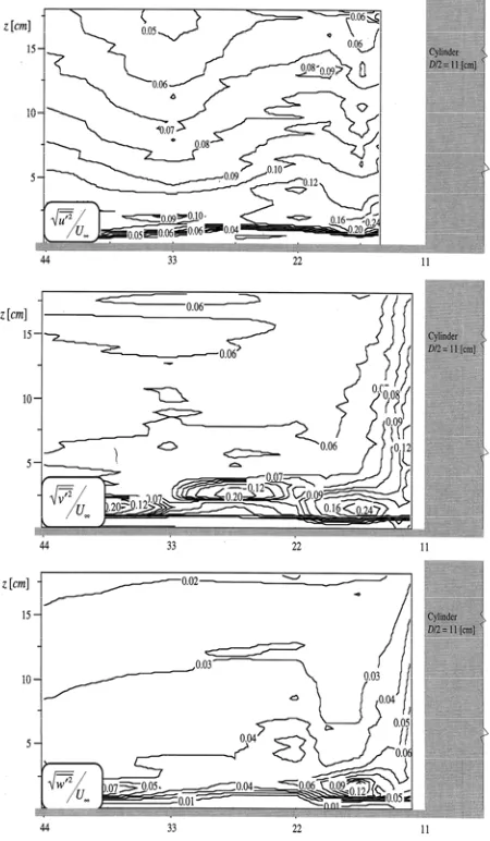
Figure 9. Contours of the dimensionless turbulence
intensities, Test 1.
Approaching the cylinder, the tendencies of the three components of the turbulence intensities, u ′ 2 , ′
v 2 and w ′ 2 , are similar; the profiles increase; this is
very noticeable at some points near the bed. The turbulence intensities are also presented as contours of the dimensionless turbulence intensities, u′2 U∞,
∞
′ U
v2
and w′2U∞, as shown in Figs.9 and 10 for Tests
1 and 2 respectively, which show sharp peaks in regions close to the leading edge of the cylinder. In front of the cylinder, the positions of the maximum turbulence intensities are in the regions of the horse-shoe vortex.
The turbulent kinetic energy (k) in the radial planes was calculated, using the following definition:
(
2 2 2)
2 1
=
u
v
w
Figure 10. Contours of the dimensionless turbulence intensities, Test 2.
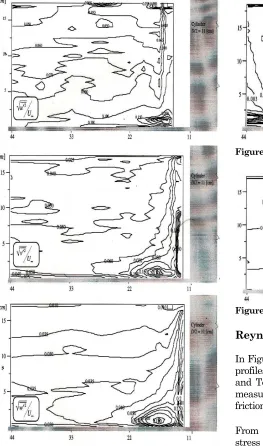
The contours of the turbulent kinetic energy are presented in Figs. 11 and 12 for Tests 1 and 2, respectively. Close to the cylinder there are regions where one composant of the turbulence was not measured, and are thus not shown. From these figures, one observes the maximum turbulence kinetic energy, max
k , for Test 1, is 0.025 m2/s2 at r/D = 0.72 and z/D = 0.06, while for Test 2, kmax is 0.020
m2/s2 at r/D = 0.73 and z/D = 0.04.
The positions of the kmax as well as the maximum
turbulence intensity, are in the regions of the vortices, a small vortex in the upstream from the cylinder.
Figure 11. Contours of the turbulent kinetic energy, Test 1
Figure 12. Contours of the turbulent kinetic energy, Test 2
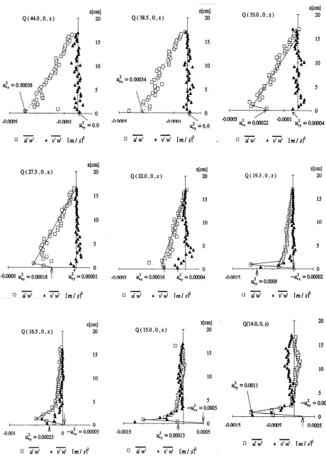
Reynolds stress profiles
In Figures 13 and 14, the measured Reynolds-stress profiles in two directions, u ' w ' and v ' w ' , for Test 1
and Test 2 are plotted. Applying the fitting to the measured data near the bed, the values of the friction velocities, u
*x and u*y, at z = 0 are obtained.
From Q (44.0, 0°, z) to Q (27.5, 0°, z), the Reynolds stress distributions have a maximum value at a certain distance close to the bed, and diminish towards a zero value at the water surface. Measurements from Q (22.0, 0°, z) to Q (14.0, 0°, z), present a significant peak at a certain level above the bed. The fitting of the data under this peak gives a negative value of the friction velocity from Q (19.3, 0°, z) to Q (14.0, 0°, z). From Q (13.0, 0°, z) to Q (12.0, 0°, z), the u ' w ' -profiles were not measured.
The v ' w ' values far upstream from the cylinder are
small and have no well defined shapes. Measurements from Q (22.0, 0°, z) to Q (14.0, 0°, z), give small values at the upper region of the water depth and increase towards the bed. At measurements close to the cylinder, from Q (13.0, 0°, z) to Q (12.0, 0°, z ), the v ' w ' distributions have a triangular
Approaching the cylinder, one observes the shear stress decreases, having the opposite direction at positions close to the cylinder. A zero value of shear stress should be at the separation point.
Conclusion
Measurements of the velocity and its turbulence intensities, upstream from a cylinder are reported for fully developed turbulent open-channel flow at ReD≈
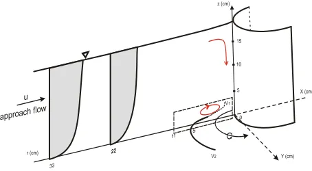
105. This flow has been documented with the mean point velocity field. The measurements were made with a non-intrusive ADVP-instrument. Based on the experiment results discussed in this paper, some findings are summaries in Fig. 15, as:
• Approaching the cylinder, the longitudinal velocities, u, decrease; their distribution becomes more uniform and close to the bed a reverse flow is noticeable with increasing importance. The downward velocity component increases, reaching
w
= 0.3- 0.35U∞ , this is clearly shown,continuing with the return flow near the bed, forming a vortex.
• At positions where the horse-shoe vortex appears in the upstream from the cylinder, a large increase of the three components of the turbulence intensities is remarked.
• The friction velocities obtained from the measured Reynolds-stress near the bed, presented a significant peak at a certain level above the bed.
• The downward flow and the vortex system play an important role, if the bed material is movable. The peak shear stress near the bed may be responsible to the bed erosion, while the vortex participates in the transportation of sediments.
z (cm)
X (cm)
Y (cm) V2
V1
r (cm)
15
10
5
0
Figure 15. Scheme of the Flow Fields Upstream of the
Cylinder
References
1. Agui, J.H. and Andreopoulos, J., Experimental Investigation of a Three-Dimensional Boundary Layer Flow in the Vicinity of an Upright Wall Mounted Cylinder, J. Fluids Engineering, Vol. 114, 1992, pp. 566-576.
2. Eckerle, W.A. and Awad, J.K., Effect of Freestream Velocity on the Three-Dimensional Separated Flow Region in Front of a Cylinder, J. Fluids Engineering, Vol. 113, 1991, pp. 37-44.
3. Eckerle and Langston, Horseshoe Vortex Formation around a Cylinder, ASME J. of
Turbomachinery, Vol. 109, April 1987, pp.
278-285.
4. Monnier, J.C. and Stanislas, M., Study of a Horseshoe Vortex by LDV and PIV, ERCOFTAC Bulletin, No. 30, 1996, pp. 19-24.
5. Pierce, F.J. and Tree, I.K., The Mean Flow Structure and the Symmetry Plane of a Turbulent Junction Vortex, J. Fluids Engineering, Vol. 112, 1990, pp. 16-22.
6. Barbhuiya, A.K. and Dey, S., Measurement of Turbulent Flow Field at a Vertical Semicircular Cylinder Attached to The Sidewall of a Rectangular Channel, Flow Measurement and
Instrumentation, Volume 15, Issue 2, April 2004,
Elsevier, pp. 87-96.
7. Yulistiyanto, B., Zech, Y., and Graf, W.H., Free-Surface Flow around a Cylinder: Shallow-Water Modeling with Diffusion-Dispersion, Journal of Hydraulic Engineering, Vol. 124 (no.4), 1998, pp. 419-429.
8. Andreas, R, Mutlu Sumer, B., Jorgen, F., and Jess, M., Numerical and Experimental Investigation of Flow and Scour around a Circular Pile, Journal
of Fluid Mechanics, 534, Cambridge, 2005, pp.
351-401.
9. Barbhuiya, A.K. and Dey, S., Velocity and Turbulence at a Wing-Wall Abutment, Sadhana,
Vol. 29, Part 1, February 2004, India, pp. 35–56.
10.Graf W.H. and Altinakar, M.S., Hydraulique Fluviale, Tome 1, Presses Poly. et Univ. Romandes, Lausanne, CH, 1993.
11.Yusron, S., Fractional Critical Shear Stress at Incipient Motion in a Bimodal Sediment, Civil
Engineering Dimension, Vol. 10, No. 2, September
2008, pp. 89-98.