Behaviour of the static pressure around a tussock
grassland–forest interface
Joost P. Nieveen, Rushdi M.M. El-Kilani, Adrie F.G. Jacobs
∗ Meteorology and Air Quality Group, Wageningen University, Duivendaal 2, NL-6701 AP Wageningen, The NetherlandsReceived 3 June 2000; received in revised form 6 November 2000; accepted 14 November 2000
Abstract
A field experiment was executed to measure static pressure differences around a forest edge. So-called ‘Quad-Disks’ were used to measure static pressure unaffected by the dynamic pressure induced by the probe itself. Flow obliquity appeared to have little influence on the results. For a smooth to rough transition, the results showed a maximum pressure difference within the forest atx=0.6 h relative to the probe atx = −4 h, where the height of the foresth=25 m. For a rough to smooth transition the normalised pressure differences were only weak. A maximum pressure difference was found just outside the forest atx=0.6 h relative to the probe atx=4 h probably related to a reattachment point. A negative pressure was present at the probe atx= −4 h. © 2001 Elsevier Science B.V. All rights reserved.
Keywords: Forest edge; Grassland–forest interface; Static pressure
1. Introduction
The composing elements of landscapes on a re-gional scale (∼10 km), such as grasslands, agricultural crops, hills, tree lines, urban areas or forests, all in-teract in their own characteristic way with the atmo-spheric surface layer. Consequently, the properties of the airflow over the landscape are constantly chang-ing in contrast to flat homogeneous landscapes. At a step change in surface or changes in scalar fluxes or concentration, the flow field is gradually adjusting to the new underlying surface. This results in: the built up of an internal boundary layer (IBL) and an equi-librium layer (EL), modified vertical profiles of wind, temperature and/or humidity and changing turbulent
∗Corresponding author. Tel.:+31-317-483981; fax:+31-317-482811.
E-mail address: [email protected] (A.F.G. Jacobs).
characteristics (Garratt, 1990). Here, we will focus on a transition in surface roughness only.
The effect of a surface roughness transition on the flow field, has been studied in both model approaches and scarce field and wind tunnel experiments. The em-phasis has been on, firstly, the growth of an IBL and the development of an EL within it to derive fetch re-quirement rules (Garratt, 1990). Secondly, on the ef-fect and design of (multiple) windbreaks often used in agriculture to alter the microclimate of crop canopies (McAneney and Judd, 1991).
Present fetch requirement rules are based on a lim-ited number of outdoor and wind tunnel experiments by e.g. Bradley (1968), Antonia and Luxton (1971, 1972), Munro and Oke (1975), Antonia and Wood (1975), Mulhearn (1976, 1978), Gash (1986), Kruijt et al. (1995) and most recently Irvine et al. (1997). The first suggested the height of the EL to be 1 or 2% of the horizontal distance from the transition. All the others, in this sense, showed a more rapid growth
dition, the static pressure field changes considerably. It is to be expected that around this surface change the static pressure field plays an important role in the turbulent exchange mechanism. Studies in which this pressure field was monitored were Jacobs (1984) who studied this static pressure field around a solid line obstacle and Wilson (1997), who studied the static pressure field around a porous windbreak.
Full understanding of the processes induced by a roughness transition and their effect on the mean flow field and turbulent characteristics of that flow field is therefore, of major importance to derive rep-resentative flux densities in micro-meteorological experiments close to transitions, optimum windbreak aerodynamics for agricultural purposes and modelling of complex terrain at a regional scale. In this frame-work, we studied the behaviour of the static pressure field in the vicinity of a tussock grassland–forest in-terface and the evolution of the pressure field with dis-tance from the interface, often neglected in numerical studies.
2. Materials and methods
2.1. Site description
The experiment took place in the winter of 1995 ei-ther side of a tussock grassland–forest interface in the “Fochtelooërveen” area, a disturbed raised bog in the north of The Netherlands (latitude 53◦00′30′′N,
lon-gitude 6◦23′52′′E and altitude
+11 m). The work was done in the framework of the surface layer integra-tion measurements and modelling (SLIMM) project
decreased towards the grassland–forest interface. At the interface the height of the trees was about 15 m. Similarly, the leaf area density increased as the vegeta-tion gradually changed from a larch forest to a mixed conifer forest. The forest was made up out of blocks of trees of different dimensions, separated by sandy roads of 5–10 m wide. During the experiment no green fo-liage was present except for the pine and fir. The fetch of both the forest and the tussock grassland reached, in the direction perpendicular to the forest edge, up to 2–3 km.
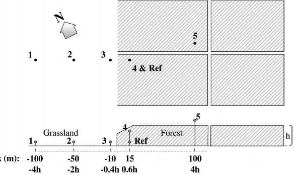
The instruments were set up in an almost straight array perpendicular to the forest edge in a NNW-ESE direction. Fig. 1 shows a top and side view of the measuring area. The black dots in the top view mark the positions of the instruments numbered from 1 to 5 and a reference, while in the side view the distance (m) from the forest edge is indicated.
2.2. Experimental set-up
Static pressure was measured using six ‘Quad-Disc’ probes (Nishiyama and Bedard, 1991) in combina-tion with a Scanivalve multiplexer (WO601/1P-12T, Scanivalve Corporation, San Diego, USA) and an ac-curate differential pressure sensor (Datametrics 590D, Datametrics Inc., Wilmington, USA). The Quad-Discs were specially designed to reject any effect of dy-namic pressure fluctuations (ρ′
= 1/2(u′)2) induced
Fig. 1. Top and side view of the experimental area. Numbers 1–5 and Ref. in the top view mark the positions of the instruments. In the side view, the distance from the forest edge and height of the forest h (=25 m) are indicated.
flasks (volume of 1 flask≈2×10⁻³m3) which acted
as a low pass filter for fluctuating pressure compo-nents (Jacobs, 1984). The container holding the flasks was efficiently insulated and painted to reduce the effect of solar heating. Internal tubes connected these ballast flasks to the multiplexer which in turn pre-sented each inlet tube sequentially to the sensor port of the differential manometer. The reference port of the manometer was connected through a similar bal-last arrangement to a probe placed at the reference position.
Measurements made by Judd et al. (1996) showed a response time of the pressure transducer to be 8 ms which was slowed by the ballast flasks (τ =0.36 s). Dynamic pressure fluctuations and the tube length between the probes and the ballast flasks showed a minimal to no effect on the response time of the dif-ferent pressure ports. The resolution of the pressure transducer was 0.05 Pa with a specified noise level of
<0.001% FS (i.e. 0.01 Pa).
The pressure probes at positions 1, 2, 3 and Ref. (see Fig. 1) were mounted on short poles 1 m above the surface. The probe at position 4 was mounted at the top of a 18 m telescopic mast, while the probe at position 5 was mounted at the top of a 27 m alu-minium mast. Next to probes 1, 2 and 3 sensitive cup anemometers (Department of Meteorology, WAU; stalling speed 0.15 m s−1) were installed at a height of
1.5 m. The 27 m aluminium mast included 3D Sonic
anemometer (Solent research, Gill Instruments Ltd., Lymington, UK). About 1 km from the forest edge in the tussock grassland, a second 3D Sonic anemometer was mounted at the top of a 8 m lattice tower.
The pressure sensor sampled at a 30 s sampling in-terval. A portable datalogger (21X, Campbell Scien-tific Ltd., Logan UT, USA) calculated 30 min averages of the mean pressure differences, mean wind speeds and wind speed S.D.
3. Results
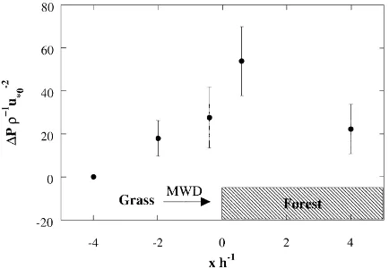
For several reasons such as periods of light winds, flat batteries or a non-rotating Scanivalve, it was nec-essary to discard some of the data. The remaining data was normalised with ρ u2∗0, where ρ is the density of the air andu2∗0 the friction velocity of the tussock grassland measured approximately 1 km away from the forest edge. Fig. 2 shows the normalised hori-zontal static pressure profiles for various mean wind directions ranging from−35 to 43◦from the
perpen-dicular, 300◦(see Fig. 1). The pressure differences do
not change much with changing incident wind for all directions except−4◦. For
−35◦there is a significant
difference for positions 4 and 5 compared to the other angles of incidence. For−4◦, a flow nearly parallel
x h−1 for a range of mean wind directions with respect to the normal (300◦) to the interface. The number in the key is the mean incident angle with respect to the normal.
small at the other positions. Judd et al. (1996) and Wilson (1997) both reported similar insensitivity to flow obliquity. In this study wind directions ranging from−25 to 25◦from the perpendicular are therefore,
regarded as normal incident flow.
3.1. Smooth to rough experiments
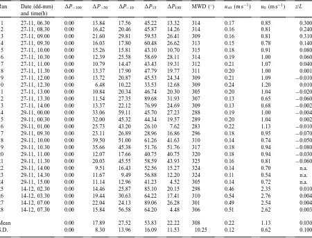
Fig. 3 displays the mean horizontal normalised static pressure profiles for 28 runs with a normal in-cident flow as described above, where the error bars indicate the S.D. of the data. Table 1 summarises
Fig. 3. Mean horizontal profile of the normalised pressure differ-ences for the tussock grassland–forest transition vs. the normalised distance x h−1. Error bars indicate the S.D. MWD: mean wind direction.
the results of those runs including the atmospheric conditions during the observations. The normalised pressure differences are relative to the pressure at position 1. For normal incident flow, Fig. 3 shows a pressure built-up towards the forest edge. The highest static pressure is found at position 4, just inside the forest. At position 5, 100 m into the forest, the static pressure drops off again, but still remains higher than the pressure at position 1.
The S.D. are rather large. Possible reasons might be the sensitivity to temperature and humidity changes inside the barometer or the relatively low wind speeds during the experimental period, with a maximum at 1.5 m of 2.8 m s−1 (u2
∗0 =0.54 m s
−1) during the 28
runs. Judd et al. (1996), who used the same equip-ment, found only an order of one unit for the S.D. of 30 runs. However, the wind speeds during their ex-periment ranged from 1 to 7 m s−1. Besides, this is
a differential measurement where the systematic (in-strumental) error of position 1 is included in the mea-surements at the other positions.
3.2. Rough to smooth experiments
Wind directions from forest to grassland were also recorded. In total 20 runs were considered reliable and were within the−25 to 25◦limits. The results of those
Table 1
The normalized pressure profiles (1P=(p−p0)ρ−1 u−∗02) either side of a grassland–forest interface for the smooth to rough runsa
Run Date (dd-mm) and time(h)
1P−100 1P−50 1P−10 1P15 1P100 MWD (◦) u∗0 (m s−1) u0 (m s−1) z/L
1 27-11, 06.30 0.00 13.84 17.56 45.22 13.32 314 0.17 0.85 0.300
2 27-11, 08.30 0.00 16.42 20.46 45.87 14.26 314 0.16 0.81 0.240
3 27-11, 09.00 0.00 21.60 29.81 59.53 26.41 309 0.16 0.81 0.310
4 27-11, 09.30 0.00 16.03 17.80 60.48 26.62 313 0.15 0.78 0.140
5 27-11, 10.00 0.00 15.26 15.81 43.10 10.70 315 0.18 0.91 0.080
6 27-11, 10.30 0.00 12.39 25.58 58.69 28.11 314 0.19 1.00 0.060
7 27-11, 11.00 0.00 10.79 14.47 43.43 19.31 312 0.21 1.07 0.040
8 27-11, 11.30 0.00 13.37 17.90 47.79 19.77 311 0.20 1.00 0.001
9 27-11, 12.00 0.00 13.72 20.87 45.53 24.34 309 0.21 1.09 −0.010
10 27-11, 12.30 0.00 6.48 10.22 33.53 12.68 309 0.24 1.20 0.010
11 27-11, 13.00 0.00 10.84 20.34 46.74 20.30 305 0.20 1.04 −0.020
12 27-11, 13.30 0.00 11.54 27.35 89.68 31.93 307 0.13 0.65 −0.060
13 27-11, 14.00 0.00 13.37 22.12 76.99 24.69 309 0.13 0.68 −0.002
14 29-11, 00.00 0.00 33.06 59.11 45.70 27.23 288 0.19 1.00 −0.004
15 29-11, 00.30 0.00 32.00 45.32 44.34 19.57 289 0.20 1.04 0.002
16 29-11, 01.00 0.00 25.73 43.20 26.10 7.62 283 0.22 1.13 −0.010
17 29-11, 09.30 0.00 23.11 26.89 28.96 16.86 296 0.18 0.95 −0.070
18 29-11, 10.00 0.00 39.50 51.00 61.26 41.63 310 0.14 0.74 −0.050
19 29-11, 10.30 0.00 35.66 45.38 51.76 51.76 317 0.18 0.94 −0.080
20 29-11, 11.00 0.00 12.07 17.66 40.75 40.75 320 0.18 0.94 −0.030
21 29-11, 11.30 0.00 20.03 45.55 58.59 43.93 325 0.16 0.81 −0.060
22 29-11, 14.00 0.00 9.51 16.43 52.56 15.27 324 0.14 0.70 n.a.
23 29-11, 14.30 0.00 11.67 9.49 56.88 12.20 324 0.11 0.54 n.a.
24 29-11, 15.00 0.00 11.14 12.96 41.23 4.52 305 0.14 0.72 n.a.
25 14-12, 02.30 0.00 14.46 25.87 85.10 20.15 298 0.46 2.35 0.010
26 14-12, 03.30 0.00 19.44 30.63 64.22 17.41 310 0.54 2.76 0.004
27 14-12, 07.00 0.00 22.04 24.13 89.06 26.28 301 0.49 2.54 0.004
28 14-12, 07.30 0.00 15.84 56.58 64.20 4.48 306 0.51 2.62 0.003
Mean 0.00 17.89 27.52 53.83 22.22 308 0.22 1.13 0.030
S.D. 0.00 8.30 13.96 16.09 11.53 10.25 0.12 0.62 0.100
aSubscripts refer to distance in metres from the grassland–forest interface. Also included are the mean wind direction (MWD), the far upstream friction velocity (u∗0), the far downstream wind speed (u0), and a stability parameter (z/L) during the observations.
to the pressure at position 5, for normal incident flow. The first thing that appears is the very weak effect on the static pressure of the transition. Static pressure dif-ferences over the same distance are one order of mag-nitude less than in the smooth to rough case. However, in both cases the flow field has probably not achieved its equilibrium yet.
Position 5, shows a small positive static pressure difference. At position 3, however, there is a small positive pressure difference while at positions 1 and 2 the static pressure differences are minor but negative. Position 3 (xh−1=0.4) could be the so-called
reat-tachment point that could explain the positive static
14 23-11, 14.30 −2.22 −0.51 1.51 0.20 0.00 109 0.54 2.78 −0.003
15 23-11, 15.00 −1.84 −0.08 2.01 −0.04 0.00 108 0.53 2.75 0.004
16 23-11, 15.30 −0.44 −0.13 2.12 −0.11 0.00 117 0.57 2.95 0.010
17 23-11, 16.00 −0.18 0.75 2.39 −0.05 0.00 99 0.58 2.96 0.010
18 23-11, 16.30 −0.56 0.07 2.40 0.00 0.00 97 0.59 3.05 0.020
19 23-11, 19.00 −1.39 −0.59 1.21 0.05 0.00 96 0.63 3.25 0.010
20 24-11, 00.30 −1.02 0.20 2.63 −0.05 0.00 110 0.67 3.47 0.010
Mean −2.35 −0.38 2.40 0.21 0.00 111 0.53 2.76 0.030
S.D. 1.94 1.19 2.83 0.70 0.00 12.75 0.13 0.68 0.043
aSubscripts refer to distance in metres from the grassland–forest interface. Also included are the mean wind direction (MWD), the far downstream friction velocity (u∗0), the far downstream wind speed (u0), and a stability parameter (z/L) during the observations.
Fig. 4. Mean horizontal profile of the normalised pressure differ-ences for the forest–tussock grassland transition vs. the normalised distance x h−1. Error bars indicate the S.D. MWD: mean wind direction.
4. Concluding remarks
We measured the static pressure about a tussock grassland–forest interface. ‘Quad Disk’ probes, in an
array perpendicular to the forest edge, were attached to an accurate differential pressure sensor. The probes showed no evidence of self induced dynamic pressure as was also found by Judd et al. (1996). However, S.D. were rather large which might partially be explained by the low wind speeds during the experiment and the sensitivity to temperature and humidity changes inside the barometer. Judd et al. (1996) found considerably smaller S.D. under higher wind speed conditions but using the same equipment and experimental set up.
Mean wind directions with angles up to 43◦from
the normal showed to have little effect on the static pressure field. To be on the safe side, mean wind di-rections up to 25◦ from the normal were considered
than in the smooth to rough case. A small positive pressure maximum was found after the forest edge that could possibly be ascribed to a reattachment point.
Acknowledgements
We would like to thank the technical staff of the Department of Physical Geography of the University of Groningen and Eddy Moors of the DLO-Staring Centre for their contribution. We are grateful to Frits Antonysen, Bert Heusinkveld, Willy Hillen and Henk de Bruin for their contribution to the field ex-periment. This project was financially supported by The Netherlands Organisation for Scientific Research (N.W.O.).
References
Altenburg, W., Jansen, H., van der Veen, W.S., 1993. Vegetatie ontwikkeling in het Fochtelooërveen van de jaren’69 to 1992. Bureau Altenburg and Wymenga, Rapport 52, Veenwouden, 53 pp.
Antonia, R.A., Luxton, R.E., 1971. The response of a turbulent boundary layer to a step change in surface roughness. Part I. Smooth to rough. J. Fluid Mech. 48, 721–761.
Antonia, R.A., Luxton, R.E., 1972. The response of a turbulent boundary layer to a step change in surface roughness. Part II. Rough to smooth. J. Fluid Mech. 53, 737–757.
Antonia, R.A., Wood, D.H., 1975. Calculation of a turbulent boundary layer downstream of a small step change in surface roughness. Aero. Quart. 26, 202–210.
Beljaars, A.C.M., Walmsley, J.L., Taylor, P.A., 1987. Modelling turbulence of low hills and varying surface roughness. Bound.-Layer Meteorol. 41, 203–215.
Bradley, E.F., 1968. A micrometeorological study of velocity profiles and surface drag in the region modified by a change in roughness. Quart. J. R. Meteorol. Soc. 94, 361–379. Elliott, W.P., 1958. The growth of the atmospheric internal
boundary layer. Trans. Am. Geophys. Un. 39, 1048–1054. Garratt, J.R., 1990. The internal boundary layer — a review.
Bound.-Layer Meteorol. 50, 171–203.
Gash, J.H.C., 1986. Observations of turbulence downwind of a forest-heath transition. Bound.-Layer Meteorol. 36, 227–237. Good, M.C., Joubert, P.N., 1968. The form drag of two-dimensional
bluff-plates immersed in turbulent boundary layers. J. Fluid Mech. 31, 547–582.
Irvine, M.R., Gardiner, B.A., Hill, M.K., 1997. The evolution of turbulence across a forest edge. Bound.-Layer Meteorol. 84, 467–496.
Jacobs, A.F.G., 1983. Flow around a line obstacle. Ph.D. Thesis, Department of Meteorology, Wageningen Agricultural University, Wageningen, 105 pp.
Jacobs, A.F.G., 1984. Static pressure around a thin barrier. Arch. Met. Geophys. B35, 127–135.
Judd, M.J.J., Predergast, P.T., Nieveen, J.P., 1996. Pressure and turbulence measurements around a windbreak: Purerua 1996. Hort Research Client Report 96/220 Rev 1.1, Kerikeri, New Zealand, 27 pp.
Klaassen, W., 1992. Average fluxes from heterogeneous vegetated regions. Bound.-Layer Meteorol. 58, 329–354.
Kruijt, B., Klaassen W., Hutjes, R.W.A., 1995. Adjustment of turbulent momentum flux over forest downwind of an edge. In: Grace, J., Coutts, M. (Eds.), Wind and Trees. Cambridge University Press, Cambridge, pp. 60–70.
Li, Z., Lin, J.D., Miller, D.R., 1990. Air flow over and through a forest edge: a steady-state numerical simulation. Bound.-Layer Meteorol. 51, 179–197.
McAneney, K.G., Judd, M.J., 1991. Multiple windbreaks: an aeolean ensemble. Bound.-Layer Meteorol. 54, 129–146. Mulhearn, P.J., 1976. Turbulent boundary layer wall-pressure
fluctuations downstream of an abrupt change in surface roughness. Phys. Fluids 19, 796–801.
Mulhearn, P.J., 1978. A wind-tunnel boundary-layer study of the effect of a surface roughness change. Rough to smooth. Bound.-Layer Meteorol. 15, 3–30.
Munro, D.S., Oke, T.R., 1975. Aerodynamic boundary layer adjustment over a crop in neutral stabilty. Bound.-Layer Meteorol. 9, 53–61.
Nishiyama, R.T., Bedard Jr., A.J., 1991. Quad-Disc static pressure probe for measuring in adverse atmospheres: with a comparative review of static pressure probe designs. Rev. Sci. Instrum. 62 (9), 2193–2204.
Peterson, E.W., 1969. Modification of the mean flow and turbulent energy by a change in surface roughness under conditions of neutral stability. Quart. J. R. Meteorol. Soc. 95, 561–575. Raine, J.K., Stevenson, D.C., 1977. Wind protection by model
fences in a simulated atmospheric boundary layer. J. Ind. Aerodyn. 2, 159–180.
Rao, K.S., Wyngaard, J.C., Cóte, O.R., 1974. The structure of two-dimensional internal boundary layer over a sudden change of surface roughness. J. Atmos. Sci. 31, 738–746.
Sawyer, R.A., 1960. The flow due to a two-dimensional jet issuing parallel to a flat plate. J. Fluid Mech. 9, 543–561.
Shaw, R., 1959. The influence of hole dimensions on static pressure measurements. J. Fluid Mech. 7, 550–564.
Shir, C.C., 1972. A numerical computation of air flow over a sudden change in roughness. J. Atmos. Sci. 29, 304–310. Vugts, H., Jacobs, A.F.G., Klaassen, W., 1994. SLIMM project.
In: Zwerver, S., van Rompaey, R.S.A.R., Kok, M.T.J., Berk, M.M. (Eds.), Studies in Environmental Science 65A, Climate Change Research: Evaluation and Policy Implications. Elsevier, Amsterdam, 674 pp.