NAVIGATION ASSISTANCE FOR ICE-INFESTED WATERS THROUGH AUTOMATIC
ICEBERG DETECTION AND ICE CLASSIFICATION BASED ON TERRASAR-X
IMAGERY
R. Ressel a , A. Frost a, S. Lehner a
a
German Aerospace Center (DLR), Earth Observation Center, Remote Sensing Technology Institute, 28199 Bremen, Germany - (rudolf.ressel, anja.frost, susanne.lehner)@dlr.de
Commission VI, WG VI/4
KEY WORDS: CFAR detector, GLCM features, iceberg monitoring, neural network, sea ice classification, TerraSAR-X
ABSTRACT:
Most icebergs present in northern latitudes originate from western Greenland glaciers, from where they drift into Baffin Bay, circulating north along Greenland coast and south along Canadian coast. Some of them drift more southwards up to Newfoundland, where they frequently cross shipping routes. Furthermore, the Arctic summer sea ice coverage significantly decreased over the last three decades. This has attracted numerous attentions from maritime end-users. To keep Arctic shipping routes safe, the monitoring of sea ice and icebergs is crucial. For this purpose, satellite-based Synthetic Aperture Radar (SAR) is well suited. Equipped with an active radar antenna, SAR satellites provide image data of the ocean and frozen waters independent of weather conditions, cloud cover or absence of daylight. In this paper, we present a processor for sea ice classification and (subsequent) iceberg detection based on TerraSAR-X imagery. In the classification step, texture features are extracted from the images and fed into a neural network, indicating areas of low sea ice concentration. Then, an adapted Constant False Alarm Rate (CFAR) detector is executed in order to detect icebergs. In the end, sea ice boundary and iceberg positions are output. Our experiments deal with HH polarized TerraSAR-X images taken in spring season in the Baffin Bay off the western Greenland coast, where both, sea ice and icebergs are present. Our results exemplify how a comprehensive ice processor with complementary information can be set up for near real time (NRT) service in ice infested waters.
1. INTRODUCTION
Due to climate warming Arctic shipping routes that were formerly impassable are becoming an option for navigation. To safeguard the travel through such ice-infested waters, reliable and up-to-date information about degree and type of ice coverage are pivotal. The discovery and extraction of natural resources in Arctic waters add yet another motivation to generate navigation assistance products for maritime users. Satellite-borne synthetic aperture radar (SAR) is well suited for this purpose, since it is available even over remote Arctic waters, independent of cloud cover and sunlight.
In this paper, we propose a new processor that is intended to assist navigation of ships in polar waters. Based on SAR data provided by the German Radar satellite TerraSAR-X (TS-X), the processor generates charted information about ice type and icebergs. The implementation is geared towards operational use with regards to processing and delivery time and format for maritime users on ships.
The following Section 2 outlines the algorithmic concept. The key ideas of the implementation for ice type classification and iceberg detection and the procedural interconnection are discussed.
This machinery is applied to TerraSAR-X images taken in spring season off the western Greenland coast, where both, sea ice and icebergs are present. We discuss experimental results in Section 3. The positive outcomes in terms of accuracy clearly indicate the power of our concept and justify increased efforts in the same direction to further improve the overall quality and operational usefulness of our processor.
2. ALGORITHMIC APPROACH 2.1 Basic concept
Sea ice classification based on SAR images has long been a focus of research ever since the advent of satellite borne SAR. Generally, the first task centers around finding suitable mathematical characterization of image portion (segments, neighborhoods). In a second step, one then attempts to find a functional relationship between such quantifiers and the different ice types. In the case of supervised classification, finding or fitting such a functional relationship is referred to as training. Such generic methods have been tested in various flavors for sea ice classification successfully (Tsatsoulis 2004, Bogdanov 2005, Breivik, 2012, Zakhvatkina 2013, Clausi 2002, Clausi 2004, Scheuchl 2003, Ressel 2014).
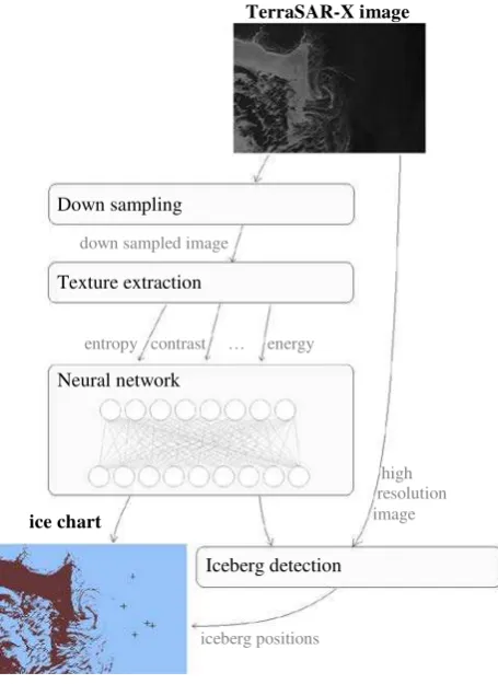
In our particular implementation, we carry out sea ice classification on a calibrated, down sampled TerraSAR-X image. From this image, texture features are automatically extracted to characterize a small neighborhood of each pixel of the image. Similarly to our former work (Ressel, 2014), the texture features of these neighborhoods are then ingested into a suitable classifier. The output of this classification process is an ice chart that depicts the dominant sea ice types in an easily comprehensible way.
2009). The concept has been used for target detection, but not for iceberg detection so far.
Finally, iceberg positions are output and added to the ice chart generated by the sea ice classification step.
Figure 1 outlines the data flow of our processor.
Figure 1. Data flow of the proposed processor
2.2 Sea ice classification
The algorithm utilizes a texture based, supervised classification approach: In a first step, for each image pixel, a vector of texture characteristics is extracted. A suitable classifier then attributes to each pixel a certain ice class, yielding an ice chart over the entire image.
The texture characterization we apply is the classical gray level co-occurrence matrix (GLCM) as described in (Haralick, 1973). Other procedures for texture description that have been applied for SAR images of sea ice are wavelets (Liu, 1991; Yu, 2002), autocorrelation features (Karvonen, 2005), and Gabor wavelets (Clausi, 2000). Due to their reported suitability for sea ice classification (Bogdanov, 2005; Zakhvatkina, 2013; Clausi, 2000) we chose these texture features for our classification procedure. For the GLCM approach, we computed for every pixel neighborhood (eg. 11x11, 31x31) of the image the histogram C(i,j) of gray level pairs of adjacent pixels. To reduce the memory consumption, 2-D histograms are computed for reduced grayscales of 4 bits, 5 bits or 6 bits. For our purposes, the reduction to 6 bits proved to be the optimal gray level degradation (see Ressel, 2015). From these histograms C(i,j), a number of statistical parameters are computed that correspond to significant visual traits of the local texture. These parameters (in our implementation we use entropy, energy, contrast,
homogeneity, dissimilarity, correlation) constitute the entries of the texture feature vector:
entropy =
∑
( )
(
( )
)
and for y respectively.
These GLCM based parameters are complemented by the local mean, local 2nd, 3rd, and 4th moment of the gray values of the pixel neighborhood.
The generation of a suitable classifier requires a training procedure prior to its application. To this end, texture vectors from images are taken where the depicted ice types are well-known. These templates of texture vectors in conjunction with correct ice type output are used to fit an ansatz function. This fitting comprises the training step. In our case we employed a neural network classifier, a statistical approach that matches the nonlinear nature of the task. The implementation relied on an open source neural network library, namely the FANN library (Nissen, 2005), which was integrated with our implementation of GLCM feature extraction.
When applying a classifier to a new SAR image with ice coverage, one has to ensure that the dominant sea ice types in the image and in the classifier match. For this reason, a library of seasonally and geographically adapted classifiers needs to be developed, from which one can then choose the most appropriate classifier for a particular image.
Containing variability of texture appearance with these precautionary measures, one can then, for example, generate a classifier trained on one SAR image and apply it to SAR images of the following days in the same region. Such classification configurations have been successfully applied on time series (Ressel, 2015) and are an appropriate method for automated sea ice charting during campaigns into ice-infested areas (eg. Lance campaign in March 2014 near Svalbard).
The incidence angle of the acquisition exhibits optimal performance for incidence angles greater than 35°. In near range and mid-range results are less reliable due to highly variable, more random texture of different ice types, in particular for open water portions.
For time critical applications, avoiding computational overhead is prioritized over higher resolution. Furthermore, scales of characteristic textures of ice types appear on a much coarser level than the full resolution would permit. For these reasons, the classification process currently implemented is carried out in reduced resolution.
Use of pre-trained classifiers for new images naturally needs a match between dominant ice types in the image and in the classifier, as well as between other mentioned side conditions (e.g. geography, season, incidence angle range). Therefore, to take these aspects into account, the deployment of a human operator with sufficient technical background for ice charting and experience with the classifier are essential for the successful application of our ice type classification product.
2.3 Iceberg detection
There are several studies on automated iceberg detection from SAR images. First and foremost, the Constant False Alarm Rate (CFAR) detector is used: From a sliding window, statistical properties of open water are estimated. Based on this estimate, pixels that yield an intensity value unusually high (compared to open water) are indicated as iceberg pixels. That is, the detector performs pixel-based thresholding. The threshold calculation relies on a constant probability of false alarm (PFA) given by the user, as well as on assumptions about the expected probability density function of the intensities in the surrounding (in our case: in open water). Generally, the threshold T is obtained by solving the relation
( )
a dawhere p(a) represents the probability density function of the surrounding intensity.
The probability density function of open water used in this work is approximated with a Log-normal distribution. Its mean µwater and standard deviation σwater are estimated from pixel values in a sliding window, which is hollow square shaped (Figure 2). Then, the threshold is calculated with the equation
water
water
k
T
=
µ
+
⋅
σ
(10)in which k denotes a design parameter that controls the PFA equivalently. Finally, a pixel is defined as part of an iceberg in case its value is greater than the threshold T. Otherwise it is defined as open water.
Figure 2. Basic principle of the CFAR detector
The CFAR detector has proven its usefulness already for ship detection (Scharf, 1991; Vachon, 1997; Brusch, 2011) and later has been applied to iceberg detection (Gill, 2001; Power, 2001). In (Buus-Hinkler, 2014), an adapted CFAR detector is utilized for detailed studies on iceberg frequency in Greenland waters. (Howell, 2004) applied the CFAR detector to dual polarized images, where each channel is processed separately. Subsequently, the detections are merged.
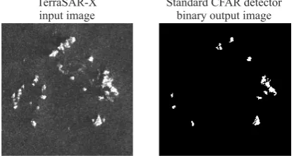
Unfortunately, the CFAR detector fails in areas of high iceberg density. As soon as a neighboring iceberg is located in the sliding window, the algorithm no longer gathers the statistical properties of open water, but of a mixture of open water and ice. In all likelihood, the values µwater and σwater, and therefore the threshold T are estimated too high. As can be seen in Figure 3, missed hits follow from this circumstance.
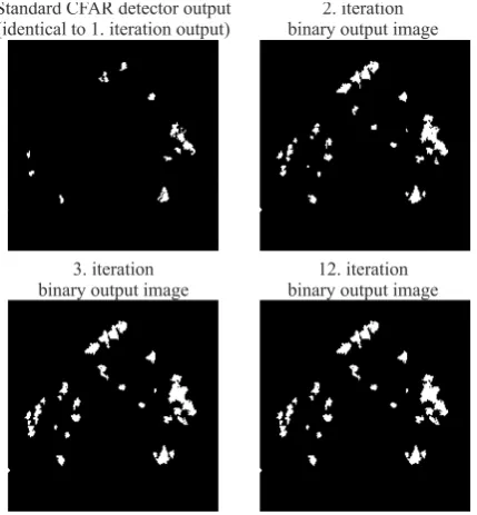
To overcome this problem, we execute the CFAR detector iteratively. In each iteration step, µwater and σwater are re-estimated. For re-estimate, we exclude pixels that have been identified in the previous iteration step to be part of an iceberg. In so doing, the new estimate is less corrupted and more iceberg pixels get detected.
In Figure 4, the iterative process is tested with the example iceberg cluster of Figure 3. After two iteration steps, all icebergs are detected. Obviously, the estimated values µwater and σwater converge towards the correct mean and standard deviation of open water pixel values. In future work, the convergence rate will be investigated.
Figure 4. Iterative CFAR detector applied to the example iceberg cluster shown in Figure 3.
In our tests shown in Section 3, the iceberg detector is carried out with two iteration steps consistently.
2.4 Fusion
The CFAR detector needs a priori knowledge about the type of intensity distribution in the surrounding of an iceberg. For open water, we approximate with a Log-normal distribution. In sea ice covered areas, however, such an assumption is inappropriate. In fact, the assumption of one single distribution type is insufficient due to high variability of different backscatter patterns for different ice types. Furthermore, the discrimination of iceberg pixels from sea ice cannot rely easily on mere thresholding i.e. the underlying assumption of CFAR that iceberg pixels lie in the tail of the intensity distribution of the surroundings does no longer hold for sea ice backscatter distributions. In sea ice, sizable portions of sea ice can have a backscatter behavior similar to icebergs.
Therefore, we apply the CFAR detector only in areas of low ice concentration, building on the output of the ice classification step (Section 2.2). The integration of the two processors is thus not merely a successive execution of both processors but the second crucially exploits knowledge from the output of the first step.
3. TEST RESULTS
The test images we discuss are taken in late spring season off the western Greenland coast. We concentrate on HH polarized TerraSAR-X acquisitions only.
The first sample image is taken in TerraSAR-X ScanSAR mode on 2014/04/21. The incidence angle for the total image ranges from 35 to 45 degrees, and for the image section shown in Figure 5 (on the left) from 40 to 45 degrees.
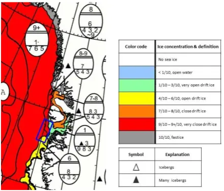
The Danish Meteorological Service (DMI) reported as daily average a wind speed of 6 m/s and a temperature between -8 °C and -12 °C without precipitation at the nearby weather station of Aasiaat. The ice situation for the preceding day (2014/04/20) is displayed in Figure 7 along with the location of the image section we processed.
The second sample image is taken in WideScanSAR mode on 2014/05/24. The incidence angle for the total image ranged from 35 to 49 degrees, for the image section shown in Figure 6 (on the left) from 44 to 49 degrees.
The DMI reported as daily average a wind speed of 6 m/s and a temperature between +8 °C and -9° C with 1 mm of precipitation at the nearby weather station of Aasiaat. The ice situation for the following day (2014/04/25) is displayed in Figure 8 along with the location of the image section.
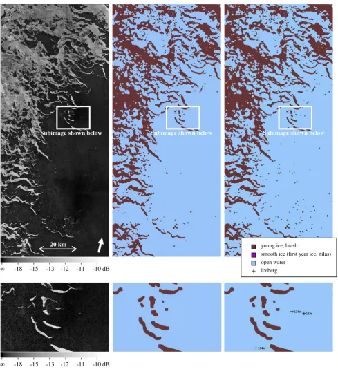
For the dominant ice types in both sample images we identified only smooth ice, which consisted mostly of first year ice floes (and some nilas), rough-surfaced ice types consisting mostly of brash and young ice floes, and open water.
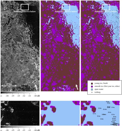
For the first image (2014/04/21), these ice types can also be discerned in the intensity images (see Figure 5, left hand side). The resulting ice chart matches the ice situation on the day before (according to the DMI ice report) quite well. In the open water portion, a low concentration of ice floes is depicted by the sparsely dispersed occurrences of ice in Figure 5. The iceberg detection algorithm automatically detects 3941 icebergs from the image. As can be seen in Figure 5 (on the bottom right) also within iceberg clusters and near to sea ice covered areas, icebergs become detected reliably due to the utilization of the iterative concept. In future work, the false alarm rate of the detector will be investigated.
The length of detected icebergs is estimated automatically. It ranges from small (15 m to 60 m) to very large (over 213 m).
Similarly, the output for the WideScanSAR image of 2014/05/24 (Figure 6) matches well the ice situation of the following day (compare DMI ice chart depicted in Figure 8). The iceberg detection algorithm outputs 2445 icebergs and size categories between small and very large.
4. CONCLUSIONS
In this paper, we proposed the process chain of an integrated sea ice classification and iceberg detection algorithm based on TerraSAR-X images. In a first step, a texture based neural network classifier identifies different ice types. During the second step of the process, icebergs are detected in the open water portions that were identified in the previous step. For iceberg detection, we employed an iterative CFAR detector.
Figure 5. Section of a calibrated TerraSAR-X ScanSAR image taken on 2014/04/21 over Baffin Bay off the western Greenland coast (left, top row), corresponding output of the sea ice classification step (in the middle, top row) and output of the processor including iceberg positions and sizes (right, top row). Color coding for ice classification: blue: open water; brown: brash, young ice; purple: first year ice, nilas. White arrows indicate direction north. The white rectangle in the top row images delineates the location of zoomed subimages in the bottom row.
young ice, brash
smooth ice (first year ice, nilas) open water
iceberg
-∞ -18 -15 -13 -12 -11 -10 dB
-∞ -18 -15 -13 -12 -11 -10 dB 20 km
Subimage shown below
Figure 6. Section of a calibrated TerraSAR-X WideScanSAR image taken on 2014/05/24 over Baffin Bay off the western Greenland coast (left, top row), corresponding output of the sea ice classification step (in the middle, top row) and output of the processor including iceberg positions and sizes (right, top row). Color coding for ice classification: blue: open water; brown: brash, young ice. White arrows indicate direction north. The white rectangle in the top row images delineates the location of zoomed subimages in the bottom row.
young ice, brash
smooth ice (first year ice, nilas) open water
iceberg
Subimage shown below
Subimage shown below Subimage shown below
-∞ -18 -15 -13 -12 -11 -10 dB
Figure 7. Ice concentration according to DMI for 2014/04/20. Egg code for segments according to WMO. The blue rectangle indicates the location of the TerraSAR-X image shown in Figure 5.
Figure 8. Ice concentration according to DMI for 2014/05/25. Egg code for segments according to WMO. The blue rectangle indicates the location of the TerraSAR-X image shown in Figure 6.
REFERENCES
Bogdanov, A., Sandven, S., Johannessen, O., Alexandrov, V. and Bobylev, L., 2005. Multisensor Approach to Automated Classification of Sea Ice Image Data. IEEE Transactions on Geoscience and Remote Sensing, 43(7), pp. 1648-1664.
Breivik, L.-A., Eastwood, S., and Lavergne, T., 2012. Use of C-Band Scatterometer for Sea Ice Edge Identification IEEE Transactions on Geoscience and Remote Sensing, 50(7), pp. 2669–2677.
Brusch, S., Lehner, S., Fritz, T., Soccorsi, M., Soloviev, A., and van Schie, B., 2011. Ship surveillance with TerraSAR-X. IEEE Transactions on Geoscience and Remote Sensing, 49(3), pp. 1092-1103.
Buus-Hinkler, J., Qvistgaard, K., and Harnvig Krane, K. A., 2014. Iceberg number density – Reaching a full picture of the
Greenland waters. Geoscience and Remote Sensing Symposium (IGARSS), IEEE International.
Clausi, D. A. and Zhao, Y., 2002. Rapid Extraction of Image Texture by Co-occurrence Using a Hybrid Data Structure, Comput. Geosci., 28(6), pp. 763–774.
Clausi, D. A. and Yue, B., 2004. Comparing Cooccurrence Probabilities and Markov Random Fields for Texture Analysis of SAR Sea Ice Imagery, IEEE Transactions on Geoscience and Remote Sensing, 42(1), pp. 215-228.
Clausi, D. A., 2010. Comparison and fusion of co-occurrence, Gabor and MRF texture features for classification of SAR sea-ice imagery. Atmosphere-Ocean, 39(3), pp. 183-194.
Gao, G., Liu, L., Zhao, L., Shi, G., and Kuang, G., 2009. An adaptive and fast CFAR algorithm based on automatic censoring for target detection in high-resolution SAR images. IEEE Transactions on Geoscience and Remote Sensing, 47(6), pp. 1685-1697.
Gill, R. S., 2001. Operational detection of sea ice edges and icebergs using SAR: Ice and icebergs. Canadian Journal of Remote Sensing, 27(5), pp. 411-432.
Haralick, R., Shanmugam, K. and Dinstein, I. 1973. Textural Features for Image Classification. IEEE Transactions on Systems, Man, and Cybernetics, 3(6), pp. 610-621.
Howell, C., Youden, J., Lane, K., Power, D., Randell, C., and Flett, D., 2004. Iceberg and ship discrimination with ENVISAT multipolarization ASAR. IEEE International Geoscience and Remote Sensing Symposium (IGARSS).
Karvonen, J., Simila, M., and Makynen, M., 2004. Open Water Detection from Baltic Sea Ice SAR Imagery. Proc. IEEE International Geoscience and Remote Sensing Symposium (IGARSS), Vol. VII, pp. 4382-4385.
Nissen, S., 2005. Neural Networks made simple. www.software20.org, 2/2005, pp. 14-19.
Power, D., Youden, J., Lane, K., Randell, C., and Flett, D., 2001. Iceberg detection capabilities of RADARSAT synthetic aperture radar: Ice and icebergs. Canadian Journal of Remote Sensing, 27(5), pp. 476-486.
Ressel, R. und Lehner, S., 2014. Texture-based sea ice classification on TerraSAR-X imagery. In: Proceedings of the 22 IAHR International Symposium on ICE 2014, Singapur, Singapur (IAHR-ICE 2014), pp. 503-509.
Ressel, R., Frost, A., and Lehner, S., 2015. A Neural Network Based Classification for Sea Ice Types on X-Band SAR Images, IEEE JSTARS, (under review)
Scharf, L. L., 1991. Statistical signal processing. Reading, MA: Addison-Wesley.
Scheuchl, B., Hajnsek, I., and Cumming, I., 2003. Classification Strategies for Polarimetric SAR Sea Ice Data, in: Applications of SAR Polarimetry and Polarimetric Interferometry, ser. ESA Special Publication, Vol. 529.
Transactions on Geoscience and Remote Sensing, 37(2), pp. 780–795.
Vachon, P. W., Campbell, J. W. M., Bjerkel, C. A., Dobson, F. W., and Rey, M. T., 1997. Ship detection by the RADARSAT SAR: Validation of detection model predictions, Canadian Journal of Remote Sensing, 23(1), pp. 48-59.